Article

A Hybrid Framework for Multivariate Time Series Forecasting of Daily Urban Water Demand Using Attention-Based Convolutional Neural Network and Long Short-Term Memory Network

1
School of Mechanical and Electronic Engineering, Wuhan University of Technology, Wuhan 430070, China
2
Hubei Digital Manufacturing Key Laboratory, Wuhan 430070, China
*
Author to whom correspondence should be addressed.
Sustainability 2022, 14(17), 11086; https://doi.org/10.3390/su141711086
Submission received: 12 June 2022 / Revised: 23 August 2022 / Accepted: 30 August 2022 / Published: 5 September 2022
(This article belongs to the Section Sustainable Water Management)

Abstract

:
Urban water demand forecasting is beneficial for reducing the waste of water resources and enhancing environmental protection in sustainable water management. However, it is a challenging task to accurately predict water demand affected by a range of factors with nonlinear and uncertainty temporal patterns. This paper proposes a new hybrid framework for urban daily water demand with multiple variables, called the attention-based CNN-LSTM model, which combines convolutional neural network (CNN), long short-term memory (LSTM), attention mechanism (AM), and encoder-decoder network. CNN layers are used to learn the representation and correlation between multivariate variables. LSTM layers are utilized as the building blocks of the encoder-decoder network to capture temporal characteristics from the input sequence, while AM is introduced to the encoder-decoder network to assign corresponding attention according to the importance of water demand multivariable time series at different times. The new hybrid framework considers correlation between multiple variables and neglects irrelevant data points, which helps to improve the prediction accuracy of multivariable time series. The proposed model is contrasted with the LSTM model, the CNN-LSTM model, and the attention-based LSTM to predict the daily water demand time series in Suzhou, China. The results show that the hybrid model achieves higher prediction performance with the smallest mean absolute error (MAE), root mean squared error (RMSE), and mean absolute percentage error (MAPE), and largest correlation coefficient (R2).

1. Introduction

Urban water demand forecasting is crucial to reduce the waste of water resources and increase environmental protection. Based on accurate water demand prediction, the water supply system can meet suitable water demand through efficient water management planning with lower energy consumption, which is a benefit for sustainable water resource utilization [1]. Moreover, the growing population and economy, together with spreading consumeristic urban lifestyles, places increasing pressure on water resources worldwide [2]. Managing daily water demand through forecasting can provide vital support to design and optimal management of water distribution systems, which is an essential part of creating a reliable, economical, and intelligent water supply system [3]. Urban water demand prediction has gained much attention, as it results in considerable economic and environmental benefits. Nevertheless, accurate prediction of water demand affected by socioeconomic determinants and climate factors, including water price, population, income growth, temperature, precipitation, and weather, is still a challenging task.
The research on water demand forecasting has been carried out for decades, and many classical algorithms and models have been developed, which can be divided into two categories in general: statistical analysis models and artificial intelligence models [4]. The statistical analysis models, such as autoregressive integrated moving average (ARIMA) [5] and multiple linear regression (MLR) [6], have successfully shown their capability in modeling long-term linear relationships of water demand time series. However, it is difficult for these conventional forecasting models to capture the nonlinear and dynamic dependence relationship between multiple variables. To deal with this problem, artificial intelligence models such as support vector regression (SVR) [7], random forest (FR) [8], and artificial neural networks (ANNs) [9] have been used in water demand prediction. Neural network models can simulate biological neural network for information processing, and they can fit the uncertainty and nonlinearity of data better than other prediction models [10]. Some novel neural network models for multivariate time series forecasting have been proposed to improve the accuracy of water demand prediction. Xu et al. [11] proposed a continuous deep belief neural network (CDBNN) model based on the chaotic theory to forecast the daily water demand time series in ZhuZhou, China. Du et al. [12] proposed a hybrid long short-term memory network (LSTM) model combined with discrete wavelet transform (DWT) and principal component analysis (PCA) preprocessing techniques for water demand forecasting, which had satisfactory performance both in catching the peaks and the average prediction accuracy. However, these neural network models still have difficulty in directly dealing with irrelevant or meaningless data points resulting from abnormal conditions or recording errors. Furthermore, Ebtehaj et al. [13] stressed the importance of preprocessing experimental data, which can result in higher accuracy of time series forecasting. Hence, there is a need to propose a more accurate neural network model that can consider correlation between multiple variables but neglect irrelevant data points for water demand forecasting.
In recent years, with the development of deep learning technologies, some classical neural network models have been successfully applied to time series forecasting, for example, a novel time series forecasting model, named SeriesNet, which can fully learn features of time series data in different interval lengths [14]. The method, based on a multilayer LSTM network by using the grid search approach, can capture nonlinear patterns in time series data for demand forecasting [15]. The recurrent neural network (RNN) can model time series reliably by learning the long-term nonlinear relationships among the sequential data. Hajiabotorabi et al. [16] presented a recurrent neural network (RNN) which was improved by using an efficient discrete wavelet transform (DWT) for predicting a high-frequency time series. Fekri et al. [17] proposed online adaptive RNN, an approach for load forecasting capable of continuously learning from newly arriving data and adapting to new patterns. Especially, an improved RNN known as LSTM has achieved excellent performance in time series tasks such as petroleum production forecasting [18], volatility forecasting [19], demand forecasting [15], and photovoltaic power forecasting [20]. However, the single LSTM model finds it difficult to effectively use the time series information in historical data to predict multivariable time series [21,22]. To overcome this shortcoming, deep LSTM networks are proposed to improve the learning ability of sequence data by combining multiple LSTM layers [23]. Different from RNN models that acquire temporal features on the sequential learning process, convolutional neural networks (CNNs) use a nonlinear filter to learn the representations among the dataset, which takes into consideration the correlation between multivariate variables [24]. Wang et al. [25] proposed multiple CNNs to efficiently extract the long- and short-period information of the multivariate time series. Furthermore, CNN models can be combined with RNN models for multiple time series forecasting. Khaki et al. [26] presented a deep learning framework using CNN and RNN for crop yield prediction based on environmental data and management practices, which significantly outperformed other popular methods such as LASSO, random forest, and DFNN. Li et al. [27] used a multivariate CNN-LSTM model to forecast particulate matter (PM2.5), which had the best results compared with the univariate LSTM model, multivariate LSTM model, and univariate CNN-LSTM model. Essien et al. [28] proposed a deep encoder-decoder architecture based on convolutional LSTM and bidirectional LSTM for multistep machine speed prediction, which enables the improvement of production scheduling and planning. Although the above studies considered the influence of multivariable historical data on prediction accuracy, they did not take into account the different contributions of multivariable historical data in different periods [29].
In order to improve the prediction accuracy of deep neural network models for multivariate time series forecasting, attention mechanism (AM) was introduced to consider the different contributions of historical data at different time to data points [30]. AM is included with the encoder-decoder networks to allocate corresponding attention according to the importance of time series at different time to data points. The attention-based neural network models have been utilized to enhance the impact of significant temporal features in time series forecasting [31]. Liu et al. [32] proposed attention-based CNN to anticipate the short-term traffic speed with considerable advantages. Ding et al. [33] applied the STA-LSTM model based on LSTM and attention mechanism to flood forecasting. The STA-LSTM model based on LSTM performed better than other classical neural network models, such as FCN, CNN, GCN, and LSTM. Liu et al. [34] presented a dual-stage two-phase attention-based RNN that was successfully applied to long-term prediction of multivariate time series. Wang et al. [35] proposed the bidirectional LSTM model based on AM and rolling update with higher accuracy, less computation time, and better generalization ability than a single model. Among these attention-based encoder-decoder networks with different neural networks as the framework, they all achieve excellent performance in multivariate time series forecasting by using attention mechanism.
To the best of our knowledge, this paper is the first to propose an attention-based CNN-LSTM model for the prediction of daily urban water demand. Firstly, the input of this model is dependent on the correlation between the standardized water consumption data and other variable sequences through the correlation coefficient. Then, the proposed model uses 1D-CNN to extract features among the multivariable time series. Afterwards, the LSTM layers learn the nonlinear information from the output of the CNN layers. Furthermore, for the sake of assigning corresponding attention according to the importance of time series at different time to data points, AM is introduced to the encoder-decoder network using LSTM networks as their building block. Finally, the proposed hybrid model is examined by actual available data composed of several daily variables of the water plant in Suzhou, China, and compared with the LSTM model, CNN-LSTM model, and attention-based LSTM. The major contributions of this paper are as follows.
(1)
We propose a novel attention-based CNN-LSTM hybrid model consisting of multiple deep learning technologies to predict daily urban water demand that is transformed into multivariate time series by the correlation analysis and max-min method.
(2)
Deep LSTM networks are used as the building blocks of the encoder-decoder network to capture the historical and future information among multiple time series affecting water demand.
(3)
The CNN layers and AM are introduced to improve the performance of the encoder-decoder network for water demand forecasting. The CNN layers can consider the correlation between multivariate time series, while AM highlights important temporal features and ignores irrelevant data points of water demand sequences.
The remainder of this paper is organized as follows. Section 2 defines the multivariate time series problem to be solved, portrays the forecasting framework of the attention-based CNN-LSTM model, and illustrates the important component and process details. The case study is described in Section 3, along with the description of model data and its processing technology, as well as model evaluation criteria. Section 4 expounds the experiments conducted by using large datasets obtained from the water plant through different forecasting models. The proposed model is evaluated and compared with other methods, and the results are discussed correspondingly. Conclusions are presented in Section 5.

2. Methodology

2.1. Problem Description

In this part, we transform the water consumption forecasting problem into a time series forecasting problem, and define the multivariable time series problem to be solved. Time series data are generally a series of values (discrete or continuous form) collected at different times. The observation interval of different types of time series data is usually different and determined by the sensor specifications. In modern water plants, water supply and other variables are recorded each hour or day, and are finally saved in the databases. The corresponding definitions of water demand prediction are listed as follows.
Problem 1 (univariate time series forecasting): The daily water consumption data have complex nonlinearity and dynamic updating, which makes it difficult to capture the complex relationship among the collected time series. Traditional water demand forecasting models often use water supply as a single input to predict the future trend of water consumption. Given a univariate water supply time series X = (x1, x2, x3, …, xt), the water demand forecasting problem is to predict the future p values of the sequence Y = (y1, y2, y3, …, yp), using the values of input sequence X. Formally, there are
Y = { y 1 , y 2 , y 3 , , y p } = M ( X ) = M { x 1 , x 2 , x 3 , , x t }
where M is the traditional univariate time series forecasting model, X is the input sequence containing t values of daily water consumption, and Y is the output sequence containing p prediction values of daily water consumption.
Problem 2 (multivariate time series forecasting): Urban water demand is affected by a series of socioeconomic determinants and climate factors. Therefore, water demand depends not only on its past values but also on other variable values in some situations. Due to the relevance and influence of other factors, forecasting daily water demand needs to consider multiple variable values at the same time step. In order to model the temporal water demand sequence, it is crucial to learn the correlation feature of the multiple variables of multivariate time series. Multivariate time series forecasting of daily urban water demand is expressed by the following formula:
y t + 1 y t + 2 y t + p = M x 1 , 1 x 1 , 2 x 1 , l x 2 , 1 x 2 , 2 x 2 , l x t , 1 x t , 2 x t , l
where M, a multivariate series forecasting model, aims to predict output target values (yt, yt + 1, …, yt + p) by learning a mapping from a sequence of input data {xi,j|i = 1, 2, …, t; j = 1, 2, …, l}. {xi,j|i = 1; j = 1, 2, …, l} and {xi,j|i = 2, …, t; j = 1, 2,…, l} mean the water demand time series and other influencing factors series, respectively; p expresses the multistep forward prediction size; l represents the number of input variables; t denotes the lookup size of history data. The details of input features are listed in Section 3.1 and Table 1.

2.2. Forecasting Framework

The overall architecture of the attention-based CNN-LSTM model is shown in Figure 1. The proposed model is mainly composed of four components: CNN, LSTM, attention component, and encoder-decoder network. Firstly, through normalization and correlation analysis, a series of variables affecting water demand are selected and integrated into a multivariate time series. Secondly, CNN layers perform two convolutional and pooling operations to extract the spatial characteristics of the input data, which leads to removing the noise and unstable components in the time series. Thirdly, the LSTM layer learns the long-term nonlinear relationships among the output of the CNN unit. Furthermore, attention-based LSTM not only considers past and future data information but also highlights the effective temporal features in time series. Fourthly, the test dataset is input into the deterministic model to predict daily water consumption values.

2.3. 1D-CNN as the Multivariable Feature Extraction Module

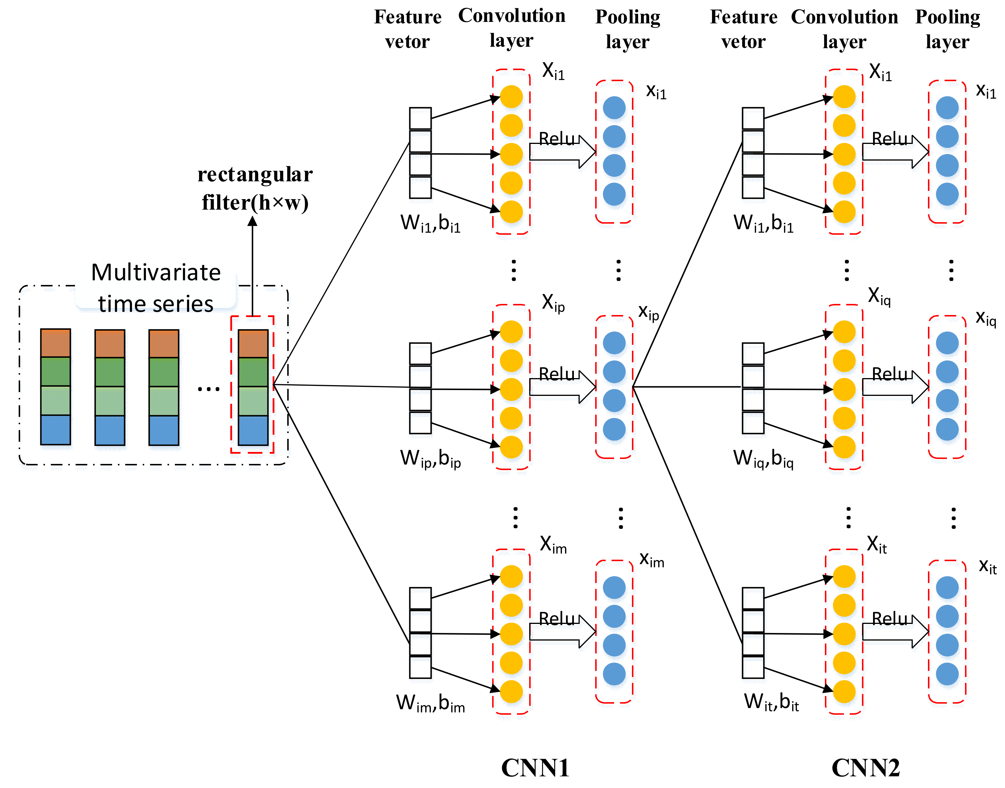
Convolutional neural networks (CNNs) are inspired by the receptive field of the animal visual cortex and are widely utilized for image processing tasks. Different from those convolutional CNNs making use of a squared filter in image processing, the one-dimensional CNN (1D-CNN) utilizes a rectangular filter to extract features of the multivariate time series. The rectangular filter’s height and width are h and w, respectively; h is the number of water consumption input vectors processed in each filter, and w represents the number of features of the input data. The 1D-CNN can accept the multivariate time series as input and extract the temporal feature through convolution layers, ReLU layers, and pooling layers. Figure 2 shows the process of 1D-CNN dealing with a multivariate time series.
When the multivariate time series is input into the 1D-CNN, convolutional layers and pooling layers of the network use sliding window to process the input. {xi,j |i = 1, 2, …, n; j = 1, 2, …, l} represents a set of water consumption input vectors of 1D-CNN. Xi,j denotes the jth variables value of the ith sample. N is the number of the training samples; l is the number of variables affecting the target value. The convolutional layer applies convolution operation to extract the original convolution features of the input data. The convolution operation can be expressed by Equation (3).
O m 1 = X i j 1 , X i j 2 ,   , X i j m 1 = Re L U ( b j 1 + j = 1 k w j 1 x i , j ) Re L U ( b j 2 + j = 1 k w j 2 x i , j ) Re L U ( b j m + j = 1 k w j m x i , j )
where O m 1 is the result of the first convolution layer processing multivariable time series; X i j m is the feature map output from the mth rectangular filter; k represents the number of convolution kernels; w j m and b j m are, respectively, the weight and the bias for the jth feature map of the mth rectangular filter.
To increase the nonlinear features of the CNN, ReLU is the activation function, which can enhance the expression ability of the network [36]. The ReLU function is defined as follows:
Re L U ( x ) = 0 ,   x 0 x ,   x > 0
The pooling layer reduces the number of parameters and network computation costs by cutting down the size of the incoming data from the convolutional layer [37]. The max-pooling reserves the maximum value from each neuron cluster in the previous layer, which is also beneficial to adjust overfitting. The max-pooling is described by Equation (5).
( x i j 1 ,   x i j 2 ,   ,   x i j m ) 1 = ( max ( j = 1 k y i j 1 ) ,   max ( j = 1 k y i j 2 ) ,   ,   max ( j = 1 k y i j m ) ) 1

2.4. LSTM as the Temporal Characteristic Extraction Block

RNNs are capable of simulating time series properly by capturing the long-term nonlinear relationships of the historical data [38]. However, standard RNNs suffer from the vanishing or exploding gradient problem when increasing the length of sequence. LSTM is a special kind of RNN with gate mechanism and memory cells, which remarkably improve the performance of RNNs. There are three kinds of gates inside each LSTM cell: input gate, forget gate, and output gate, and these gates determine the state of each memory cell through using sigmoid as the activation function to make information transmit selectively. The memory cell retaining the long-term status ct is the key structure of each LSTM cell. The internal structure of a single LSTM cell is shown in Figure 3.
Equations (6)–(8) describe the operation of the three gates for the input of each LSTM unit. Equations (9)–(11) suggest the cell states ct and the hidden states ht of each LSTM unit at time t.
i t = σ ( W i · [ h t 1 , x t ] + b i )
f t = σ W f · h t 1 , x t + b f
o t = σ ( W o · [ h t 1 , x t ] + b o )
c t = tanh ( W c · [ h t 1 , x t ] + b c )
c t = f t c t 1 + i t c t
h t = o t tanh ( c t )
where Wf, Wi, Wc, and Wo represent the weight matrices of LSTM; bf, bi, bc, and bo denote the bias vector of LSTM; ft, it, and ot are forget gate, input gate, and output gate vectors at time t; ct−1 and c t mean, respectively, the previous cell state and a new candidate value. σ(z) and tanh(z) are utilized as the activation functions, as shown below:
σ ( z ) = 1 1 + e z
tanh ( z ) = e z e z e z + e z

2.5. Attention-Based Encoder-Decoder Network of Feature Learning Module

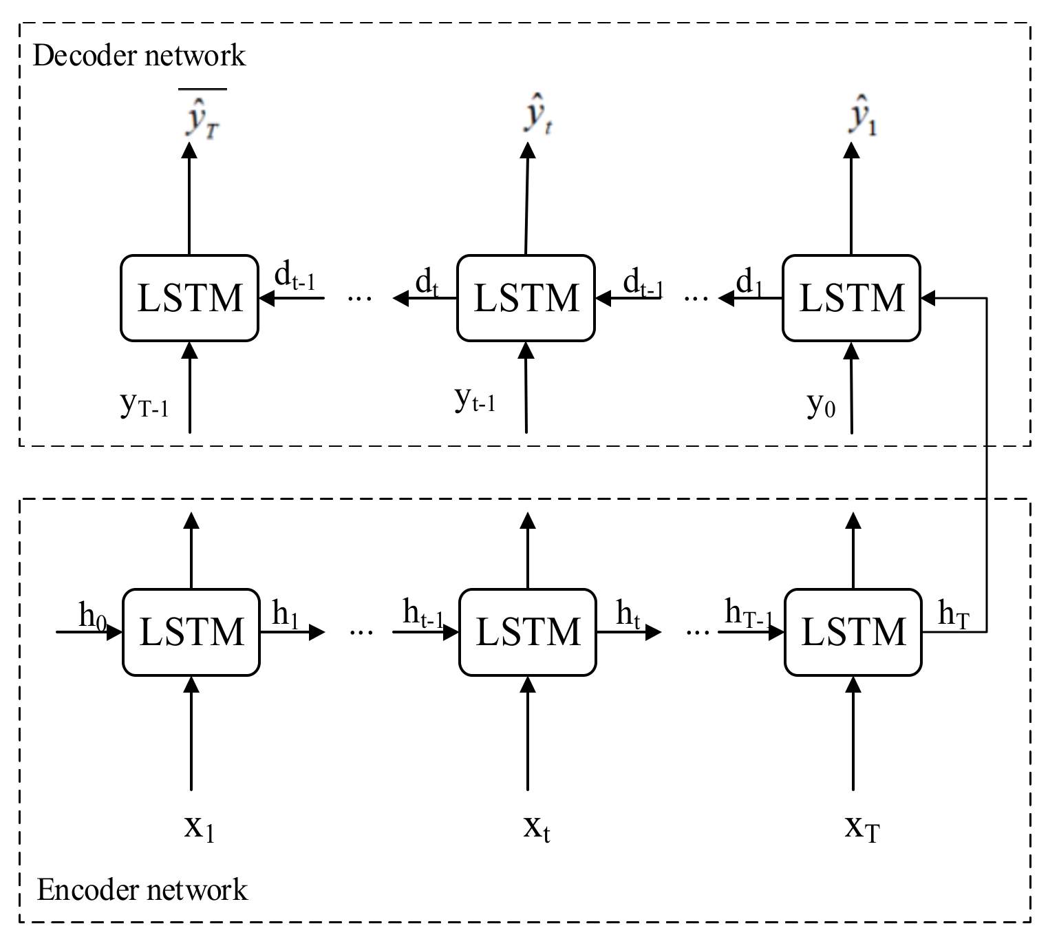
The encoder-decoder network is widely used in machine translation, which encodes the source sequence into a fixed-length vector and generates the translation using the decoder network [34]. With its excellent performance in the text translation field, the encoder-decoder network has been applied to effectively deal with the challenging sequence-to-sequence prediction problems recently [39]. Time series forecasting tasks generally involve the framework: a sequence of one or multiple input time steps converted to a sequence of one output time step. In order to consider past and future data information, the Bi-LSTM network is selected as the structural blocks of the encoder-decoder network to process sequence data. From the perspective of the model architecture, the encoder LSTM encodes the input sequence into a fixed-length vector, and the decoder LSTM decodes the fixed-length vector and outputs the predicted sequence. The structure of the encoder-decoder network based on deep LSTM networks is shown in Figure 4.
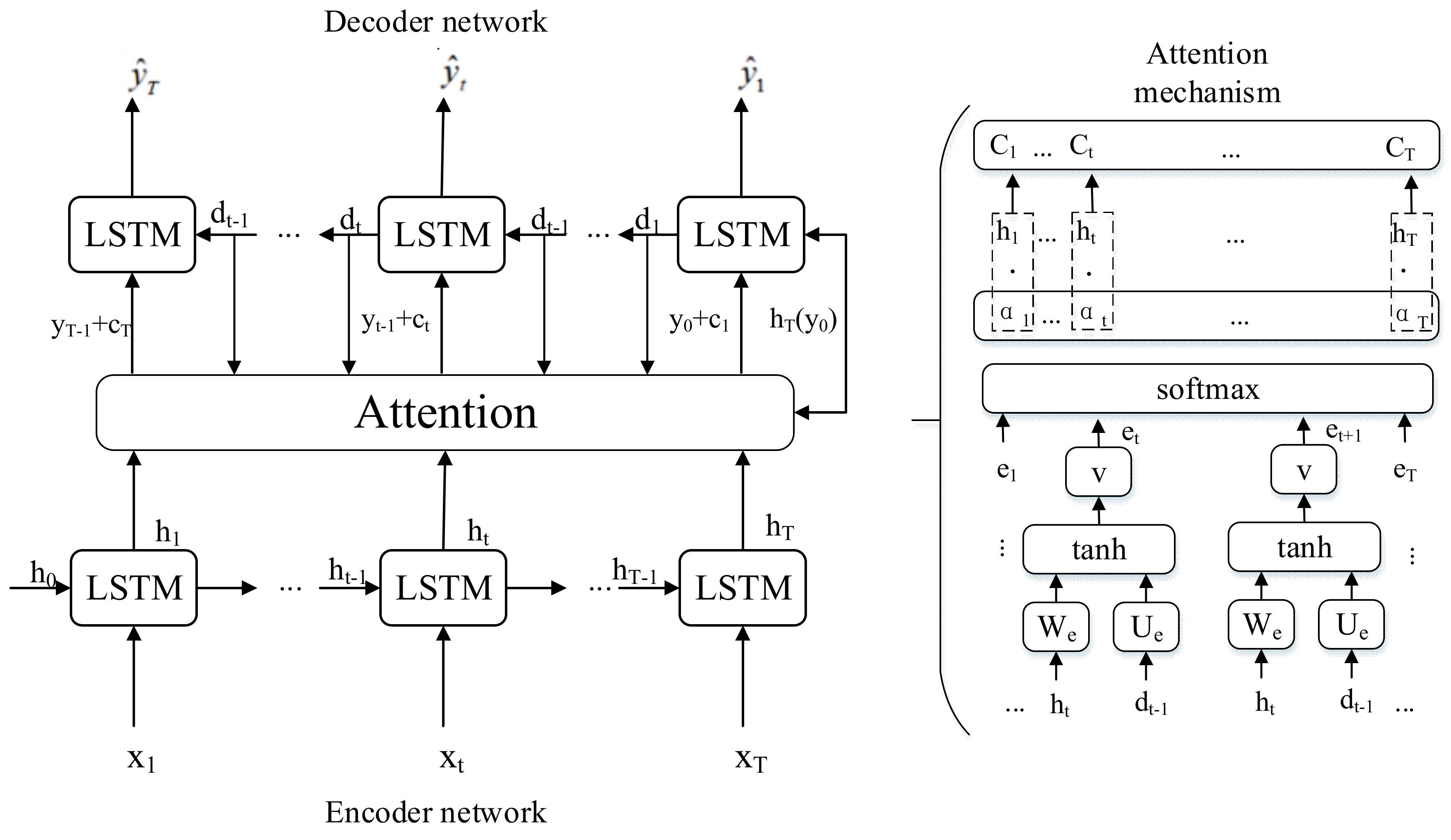
Attention mechanism (AM) comes from the simulation of attention characteristics of the human brain [35]. The core idea of AM is to allocate corresponding attention according to the importance of information, which greatly improves the reception sensitivity and processing speed of information in the concentration area. AM is commonly used to optimize the sequence processing model by allocating correlative attention weight to the features extracted from the input sequence [33]. Since the encoder-decoder network fails to work well in predicting long sequences, AM is introduced to generate a vector based on a weighted sum of all the encoded information [37]. The encoder LSTM generates the encoding information sequence {h1, h2, …, hT} from the input sequence {x1, x2, …, xT}. The decoder LSTM takes the {hT, hT−1, …, h1} and output { y ^ 1 , y ^ t , …, y ^ T }, which is the predicted sequence. AM is used to allocate corresponding attention weight to the input features at different time. The architecture of the attention-based deep LSTM model is shown in Figure 5.
et is the attention score, which is determined by the relevancy between ht and dt−1, and αt and Ct are the attention weight and weighted feature of the ith element of input datasets, respectively. The process of attention value calculation is described by Equations (14) to (16).
e t = v t · tanh W e · h t + U e · d t 1 + b
α t = exp ( e t ) t = 1 T exp ( e t )
C t = t = 1 T α t · h t
Once Ct is computed, the decoder LSTM takes Ct and dt−1 as the input to output y ^ t , which is the predicted water consumption value at the time t. Wd and bd represent the weight matric and bias vector of the decoder LSTM.

3. Application Example

3.1. Data Description

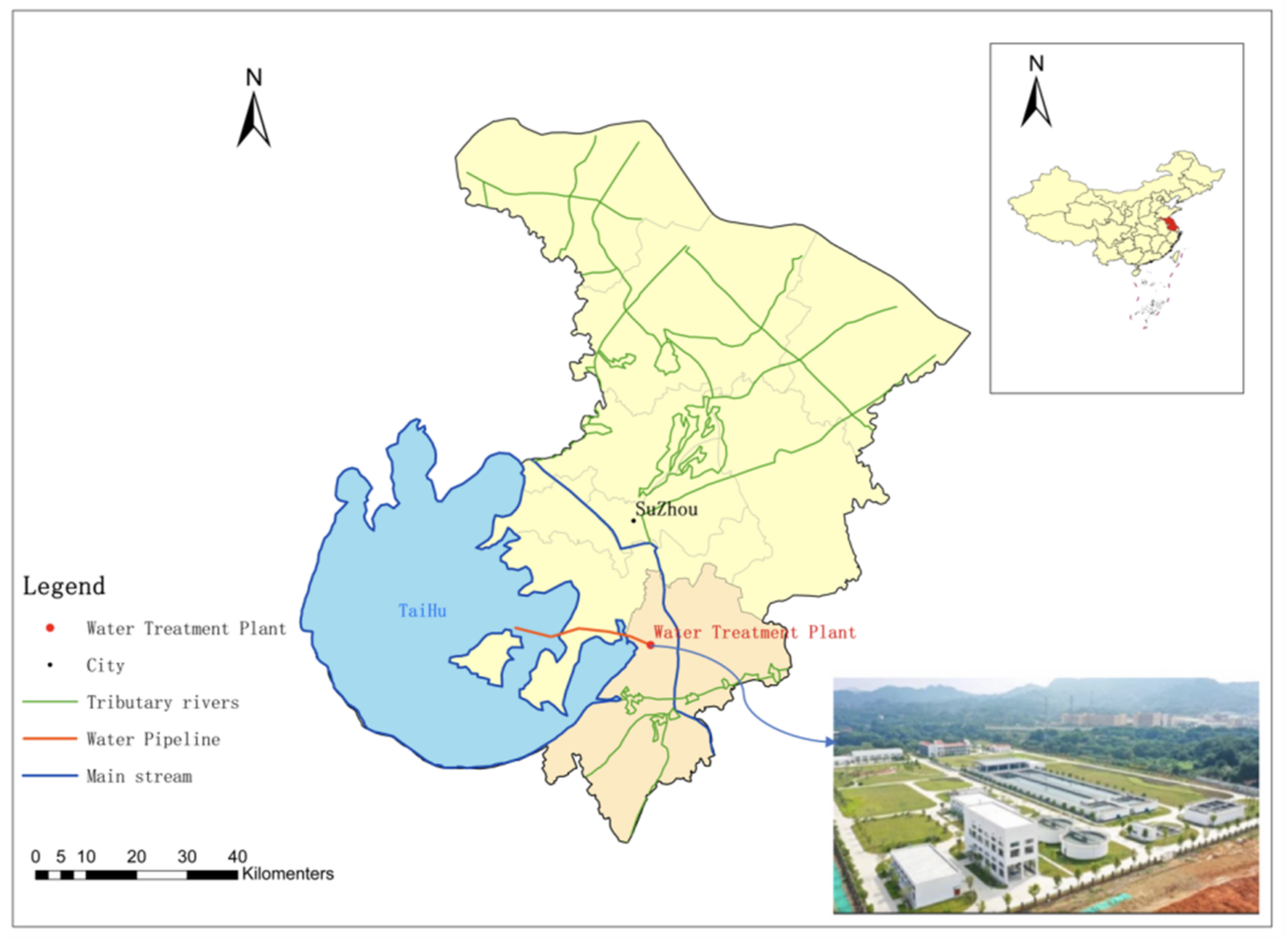
For the purpose of this study, one water plant in China, in the city of Suzhou, was utilized to develop the water demand model. The water plant, in Figure 6, takes the Taihu Lake as the water source and adopts regional water supply mode. Its water supply pipeline is 4200 km long, realizing the networking water supply of the whole city. The water supply area is about 1176 square kilometers. The annual water supply volume is 220 million cubic meters, which supplies water for about 510,000 urban residents. The daily water demand and other variables for 1674 days from 1 January 2016 to 31 July 2020 were collected from the water plant in Suzhou city. These data consist of consumption data, meteorological data, and date data, as shown in Table 1.
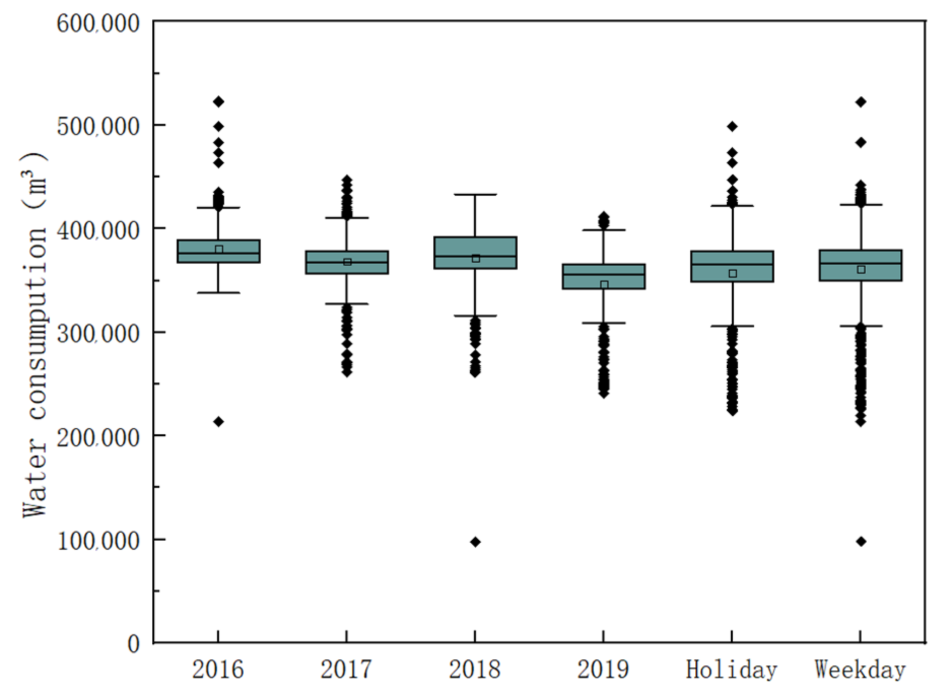
In urban water supply systems, water consumption generally includes domestic water for residents, production water for industrial and mining enterprises, and public utilities. The water demand of users does not change dramatically; however, due to some special circumstances, such as water pipe break, pipe network change, etc., these factors will cause the water supply company to stop temporarily supplying water to a certain area. In some cases, users’ special requirements for water will increase water supply. Figure 7 depicts the distribution of water demand in different years and during holidays and working days. It can be seen from the figure that the water demand data in these different ranges have almost the same mean value and median, but there is a large difference in the distribution of outliers.
The water demands in different months show some changes, most of which are affected by climate change. Figure 8a shows the average daily water consumption of each month in 2016, 2017, 2018, and 2019. It can be seen that water demand changes regularly in different months of the three years. As expected, the maximum water consumption usually occurs during hot seasons, such as July and August. In addition, Figure 8b shows that there is a relatively obvious relationship between daily water consumption and daily temperature in August 2016.
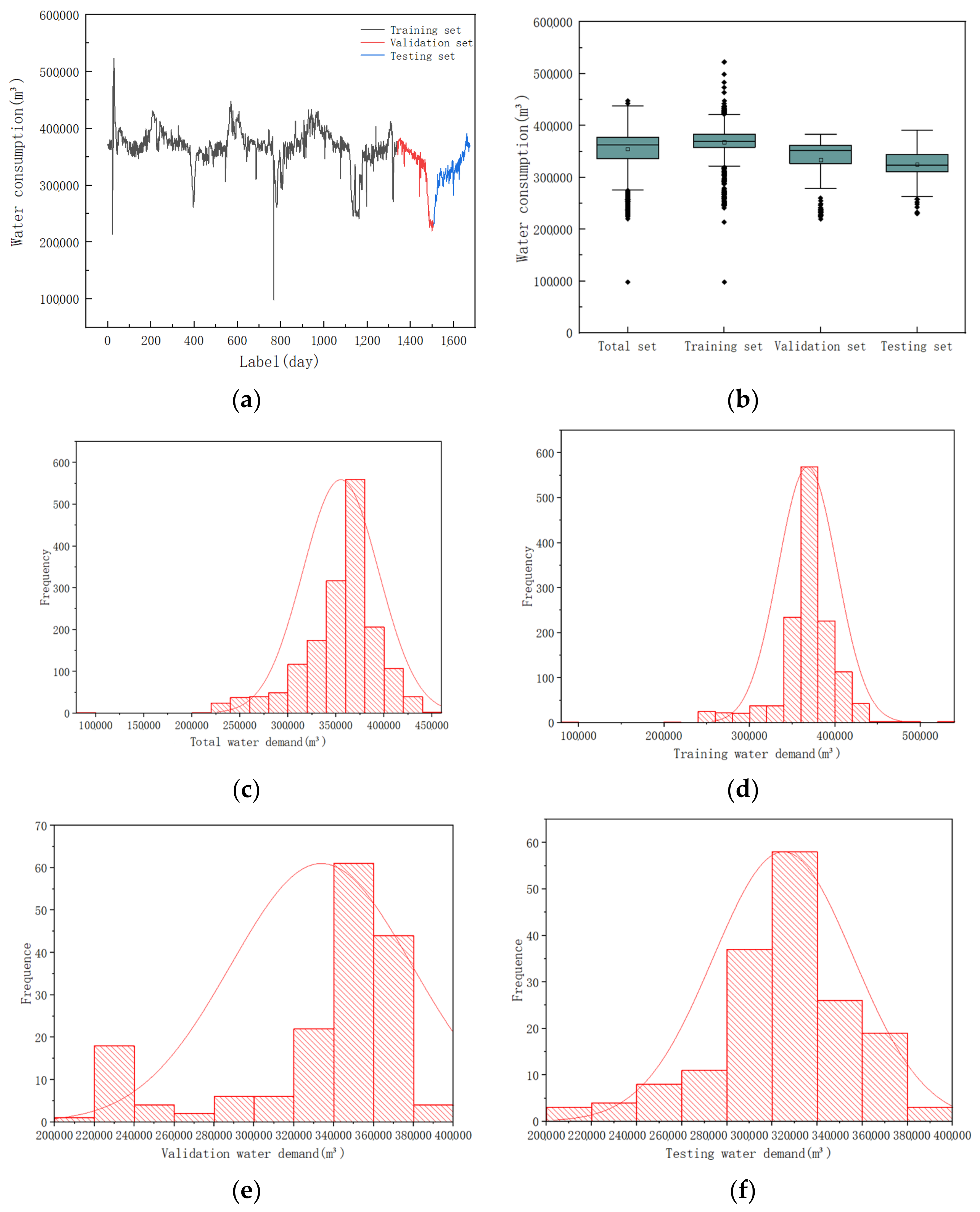
Data division is a significant process that needs to be addressed in the LSTM network. The obtainable data is generally divided into training subset, validation subset, and testing subset. These three subsets must have the same pattern, which gives LSTM network the ability to learn the historical data. In this study, our water demand data are divided into training set, verification set, and test set according to the ratio of 8:1:1. Figure 9 describes the plots of water demand time series for training, validation, and testing period alongside statistical characteristic charts.

3.2. Preprocessing Techniques

(1)
Normalization
In order to compare and weigh variables of different sizes and units, these data need to be normalized to values between 0 and 1. This approach is able to improve the efficiency of prediction and prevent the overflow occurrence of individual data during the calculation process [35]. All the collected historical data need to be normalized to facilitate subsequent analysis and processing. In this study, min-max normalization was utilized, and its calculation formulas is as follows:
x i j = x i j x j min x j max x j min
y i = y i y min y max y min
where xij and xij are the normalized and original values of the jth input variable of the ith input sample, respectively. yi and yi are the normalized and original values of the ith output sample, respectively. xjmin and xjmax are the minimum and maximum values of the jth input variable of all ith put samples, respectively. ymin and ymax are the minimum and maximum values of all output samples, respectively.
(2)
Selection of explanatory variables
With regard to water demand prediction, the selection of suitable explanatory variables as model input data has a great influence on evolving an appropriate forecast model. On the one hand, selecting variables that have a great impact on water demand as input data can improve the performance of the prediction model. On the other hand, the number of variables selected determines the number of CNN’s input nodes, thus affecting the structure of the proposed model.
Our purpose is to predict water demand in this study. Based on the previously normalized historical daily data, correlation analysis was applied to quantify the correlation effects between water consumption data at a certain time and other variable data. The process of selection of explanatory variables is as follows.
In the first stage, Pearson correlation coefficient was employed to analyze the correlation among different daily data. The normalized water demand data was divided into seven datasets with the same length. Among them, L(d) represents the daily water demand dataset, and L(d − n) denotes the corresponding daily water demand dataset of the previous n days, respectively. The Pearson correlation analysis results between the water consumption of the previous n days and that of the current day are shown in the Table 2.
It can be seen from Table 2 that the water consumption value of the latest day has the strongest correlation with that of the current day. With the increase of interval days, the correlation between the historical water consumption data and the water consumption of the day is decreasing. Therefore, the water consumption data of the latest day is selected as the input to predict the current daily water consumption.
In the second stage, Spearman correlation coefficient was utilized to analyze the correlation between normalized consumption data and other factors data. The water consumption is affected by a series of factors such as socioeconomic determinants and climate. Through correlation analysis, the impact of these collected influential factors data on water demand is quantitatively expressed. The Spearman correlation analysis results between the historical water demand data and other collected influential factor data are shown in Table 3.
It can be seen from Table 3 that there is a clear correlation among L, Max-T, Min-T, and M-label. By analyzing the correlation results of the collected data of various factors, the highest temperature, the lowest temperature, and months have a greater impact on the water demand than the weather and holidays. Therefore, the dataset composed of L, Max-T, Min-T, and M-label was chosen to predict the daily water demand.
In the final stage, based on the previous correlation analysis results, the variables with strong correlation with current water demand were selected as the input data of the model. L, Max-T, Min-T, and M-label of the latest day were designated as the input of the model to forecast the daily water consumption.

3.3. Experimental Setup

The experimental programming language was Python 3.7 and the programming software was Jupyter Notebook. The experiment was carried out on a personal computer with an Intel Core i7-7700 (2.80 GHz) CPU, 8 GB of memory, and Microsoft as 64-bit Windows 10 ultimate operating system. Our attention-based CNN-LSTM model was developed with Keras 2.3.1, which is a high-level neural networks API running on the top of TensorFlow.
The selection of model structural parameters is the key to establishing a good training model. The parameters of the deep learning model and method are mainly divided into elementary parameters and super parameters. The elementary parameters, such as weight matrix W and bias b, are determined by random initialization. The super parameters, such as layers and layers size, are confirmed by adjusting parameters several times to choose the best result. The proposed model mainly includes two CNN layers (two convolutional layers and two pooling layers), three LSTM layers, one attention layer, and three dropout layers. The dropout layers were appended to randomly delete half of the data after each processing, which reduces the data processing scale and prevents overfitting. Based on the previously selected variables, the size of the model input window was 1 × 4 (the step size was 1, the number of features was 4). The Adam optimizer was utilized to adjust the parameters in the model training process with a learning rate of 0.001 and the loss of indicator MAPE.
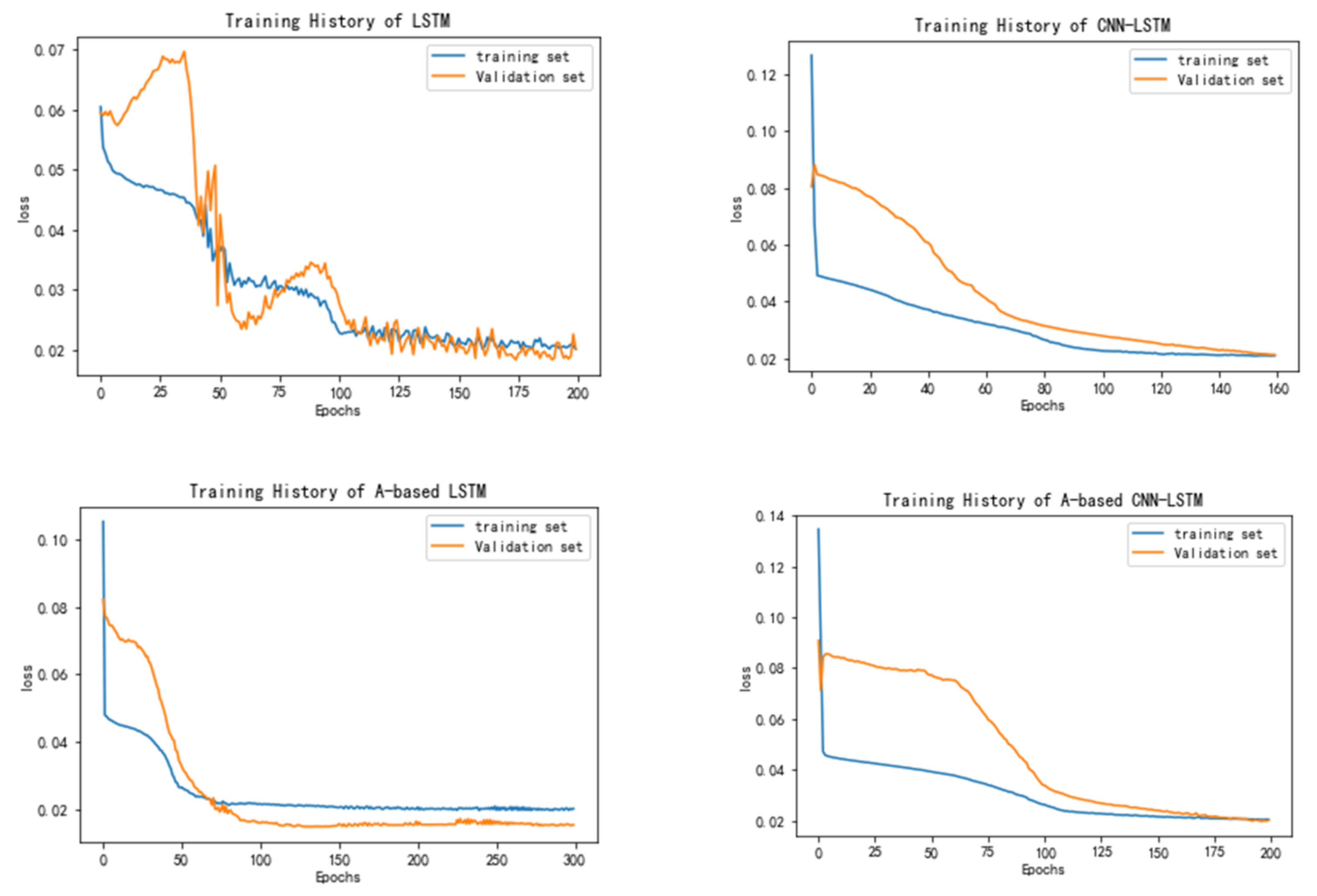
In order to verify that the ensemble learning can improve the prediction performance of the proposed hybrid attention-based CNN-LSTM model (A-based CNN-LSTM), we conducted comparison experiments using the LSTM model, CNN-LSTM model, and attention-based LSTM (A-based LSTM). The main parameters of the four forecasting models are shown in Table 4. These models used the same previously processed variables to predict the water demand in the same 100 days, respectively. The training histories of different models are shown in Figure 10.

3.4. Evaluate Criterions

The statistical criteria parameters provide a method to measure prediction accuracy, so prediction errors have great influence on the choice of suitable models and in providing insights in advising alterations to present models to minimize deviations in future predictions [40]. Several evaluation metrics were used to judge the models’ performance, such as mean absolute error (MAE), root mean squared error (RMSE), mean absolute percentage error (MAPE), and correlation coefficient (R2). The definitions of the indicators are
M A E = 1 N i = 1 N y i y ^ i
R M S E = 1 N i = 1 N y i y ^ 2
M A P E = 1 N i = 1 N y i y ^ i y i × 100 %
R 2 = 1 i = 1 N y i y ^ i 2 i = 1 N y i y ¯ 2
where N is the number of data series, y ¯ is the means of actual water consumption, p is the number of feature, and yi and y ^ i are the actual water consumption and prediction demand at time t, respectively.

4. Results and Discussions

4.1. The Prediction Results of Different Models

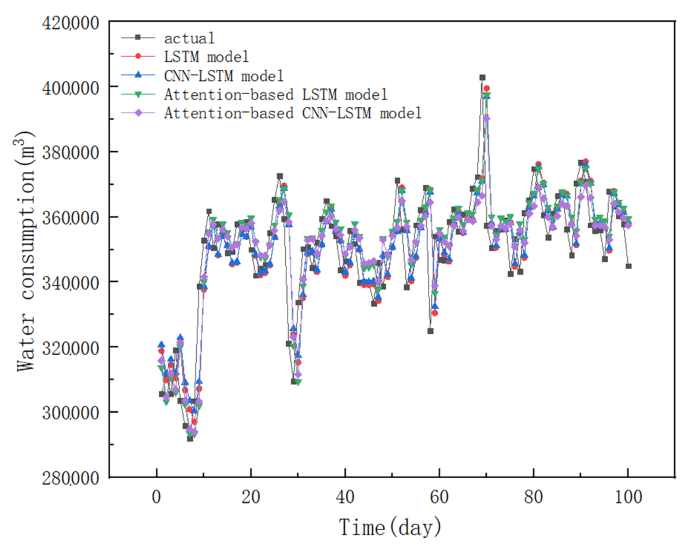
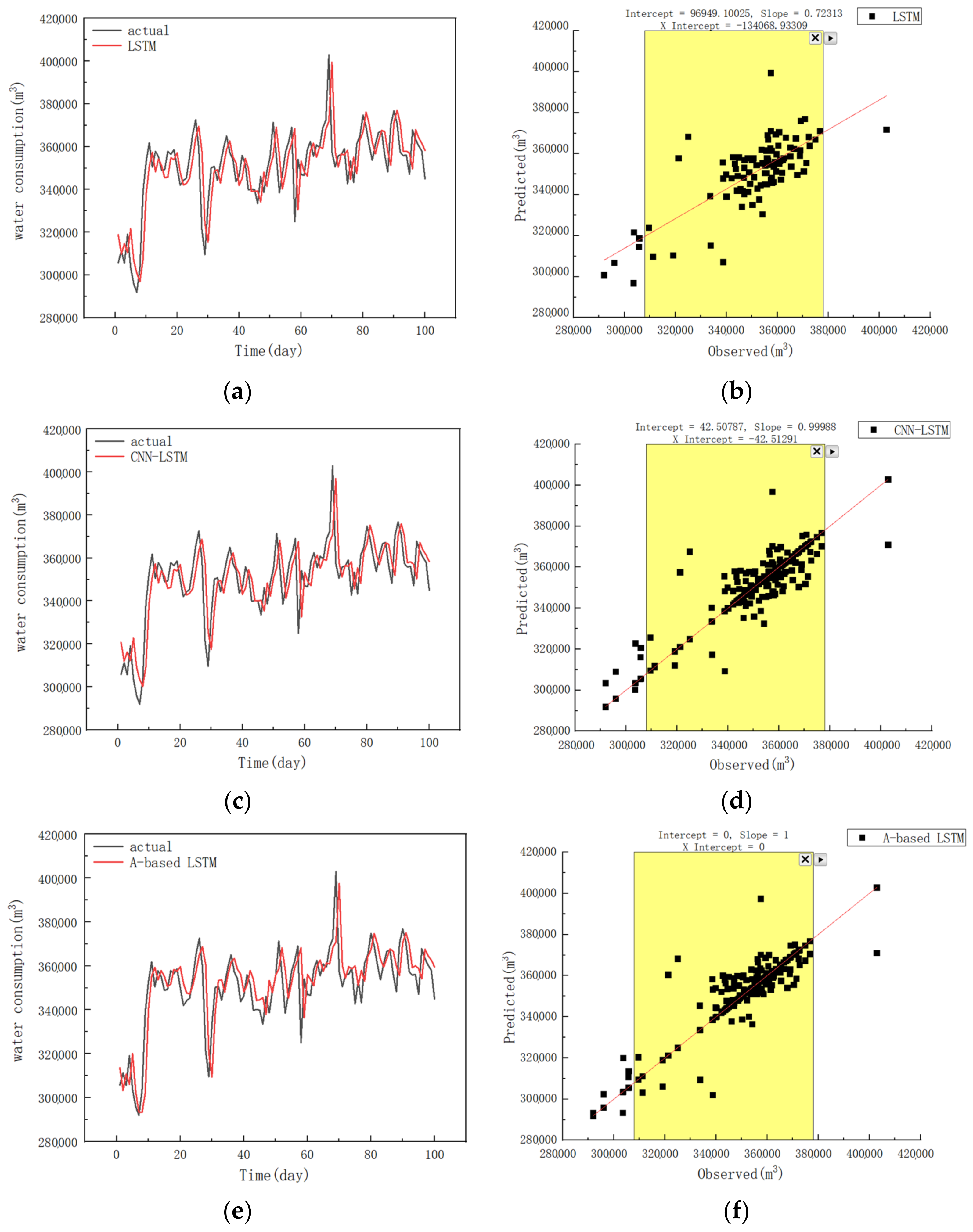
In order to verify the effect of the proposed attention-based CNN-LSTM model, LSTM model, CNN-LSTM model, and attention-based LSTM model were selected for compassion, predicting the load values in the same 100 days, respectively. The performance comparison of actual consumption and predicted values of these four models is shown in Figure 11. The forecast trends of the four models are all close to the real trend. For some peak values of actual water demand, it can be found that the prediction value of the LSTM model is the closest, and then attention-based LSTM model, CNN-LSTM model in turn. Compared with the other three models, the hybrid model proposed in this paper has the lowest sensitivity to individual peaks.
Box plots were used to analyze the data distribution of the actual water demand and the predicted water demand for each model. Figure 12 displays the box plots based on actual values and predictive values of different models. In terms of the overall data distribution, the predicted water demand of LSTM model is basically consistent with the actual water demand. Compared with other models, the distribution of water demand predicted by the attention-based CNN-LSTM hybrid model is more concentrated. However, the median and mean predicted by the proposed hybrid model are close to the actual values.
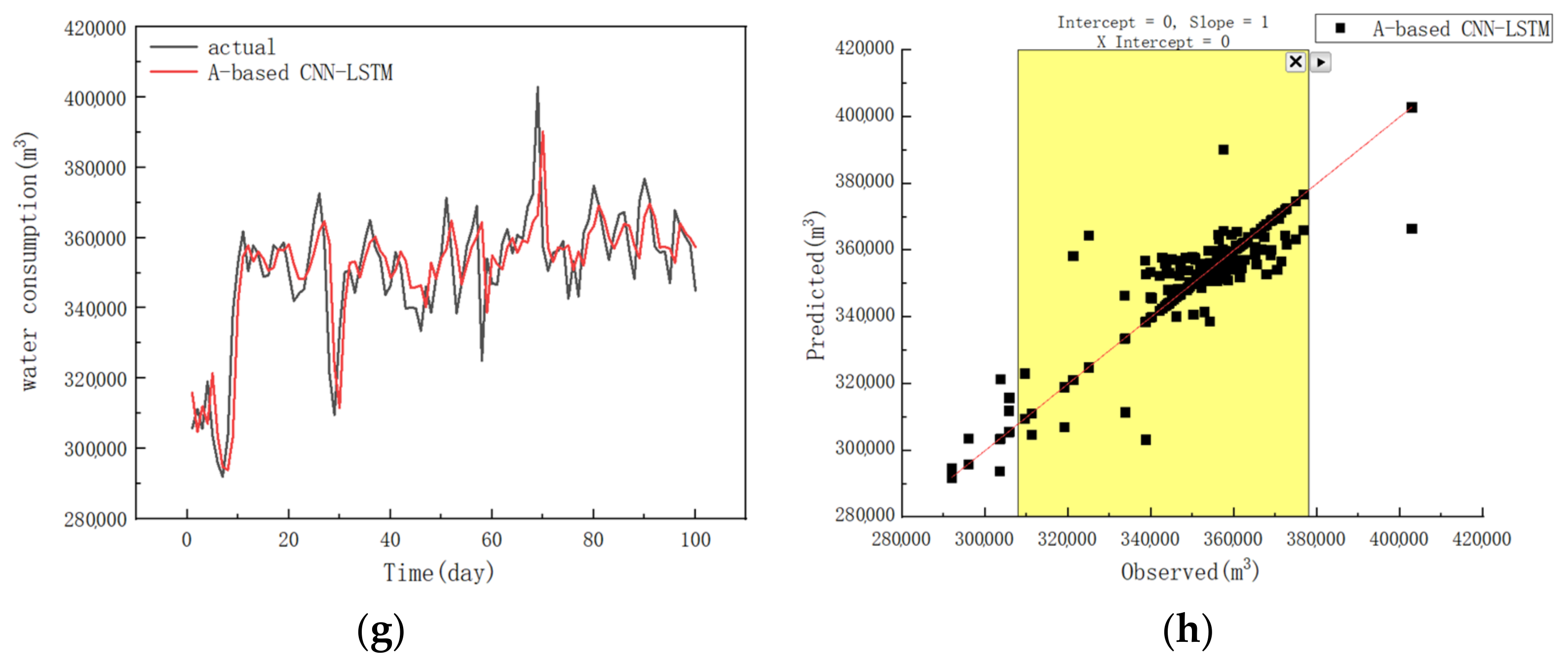
In order to further describe the prediction effect of four models on each data point, the prediction results and scatter plots of each model for 100 days of water consumption are shown in Figure 13. Figure 13a,c,e,g indicate that the predicted values of each model follow the changes of actual water consumption. It can be seen from Figure 13b,d,f,h that the prediction accuracy of each model for a few outliers is low, and there are linear relationships between the observed values and the predicted values of each model. Moreover, the correlation between the observed values and the predicted values of the attention-based CNN-LSTM hybrid model is the strongest, followed by the attention-based LSTM model and CNN-LSTM model. The LSTM model, which is sensitive to the peak values, has the worst correlation between the predicted and observed values at each time point.
For the sake of accurately evaluating the prediction performance of different models at each data point, the percentage relative error of the actual values and the predicted values were calculated as follows:
δ t = y i y ^ i y i × 100 %
where y i and y ^ i are the actual and predicted water consumption value at time t, respectively.
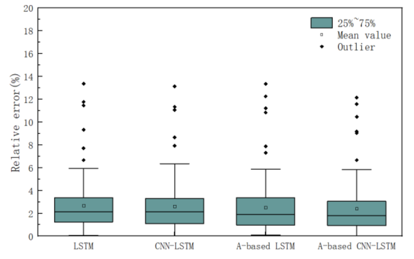
Figure 14 exhibits the relative errors distribution of each model in the same 100 points. From Figure 14, it can be easily seen that the percentage relative error of the four models for each time point data is mostly less than 6%. This reveals that the proposed model has the lowest outlier value compared with other models. In addition, the proposed model demonstrates better performance than other models in terms of the maximum, the median, and the minimum of error. Furthermore, the proposed model ensures more stable ability through a smaller distance between Q1 and Q3.
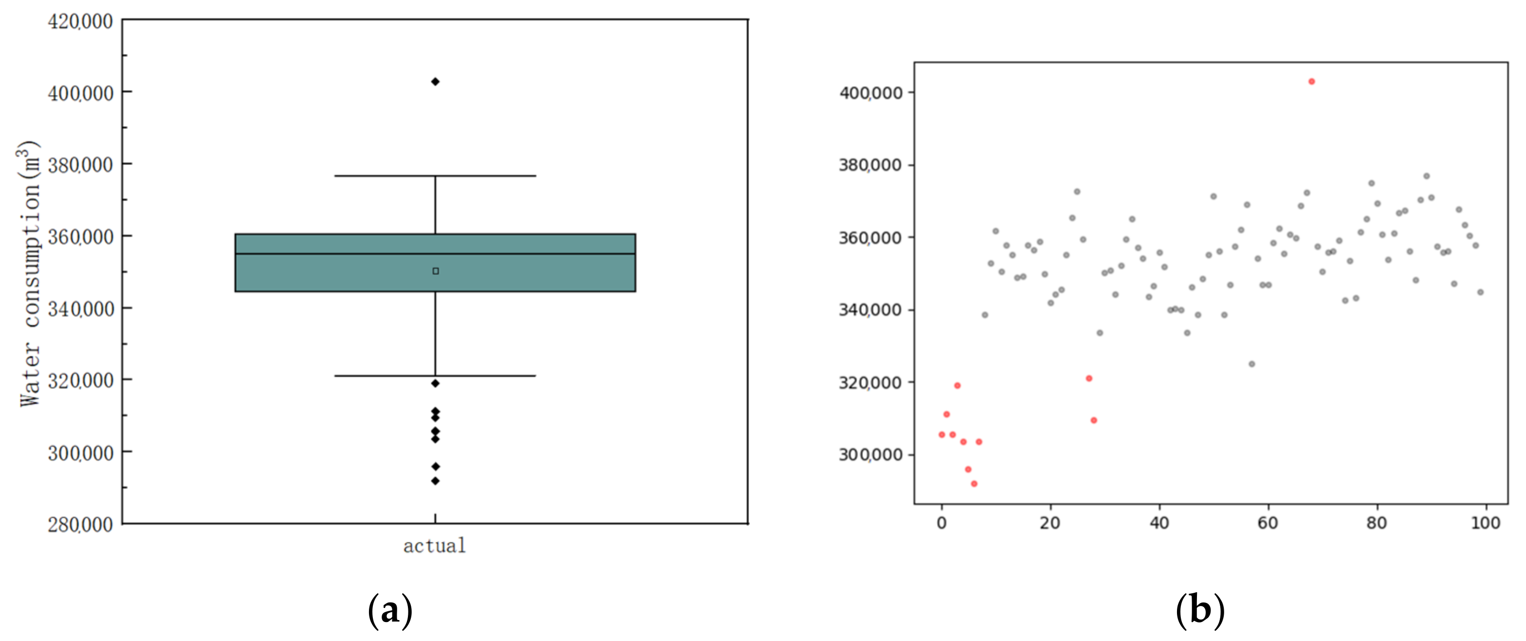
The number and location of outliers were determined by data analysis based on the box plot of 100 real water demand values. Figure 15 shows the distribution of these abnormal data in the 100 days of water consumption.
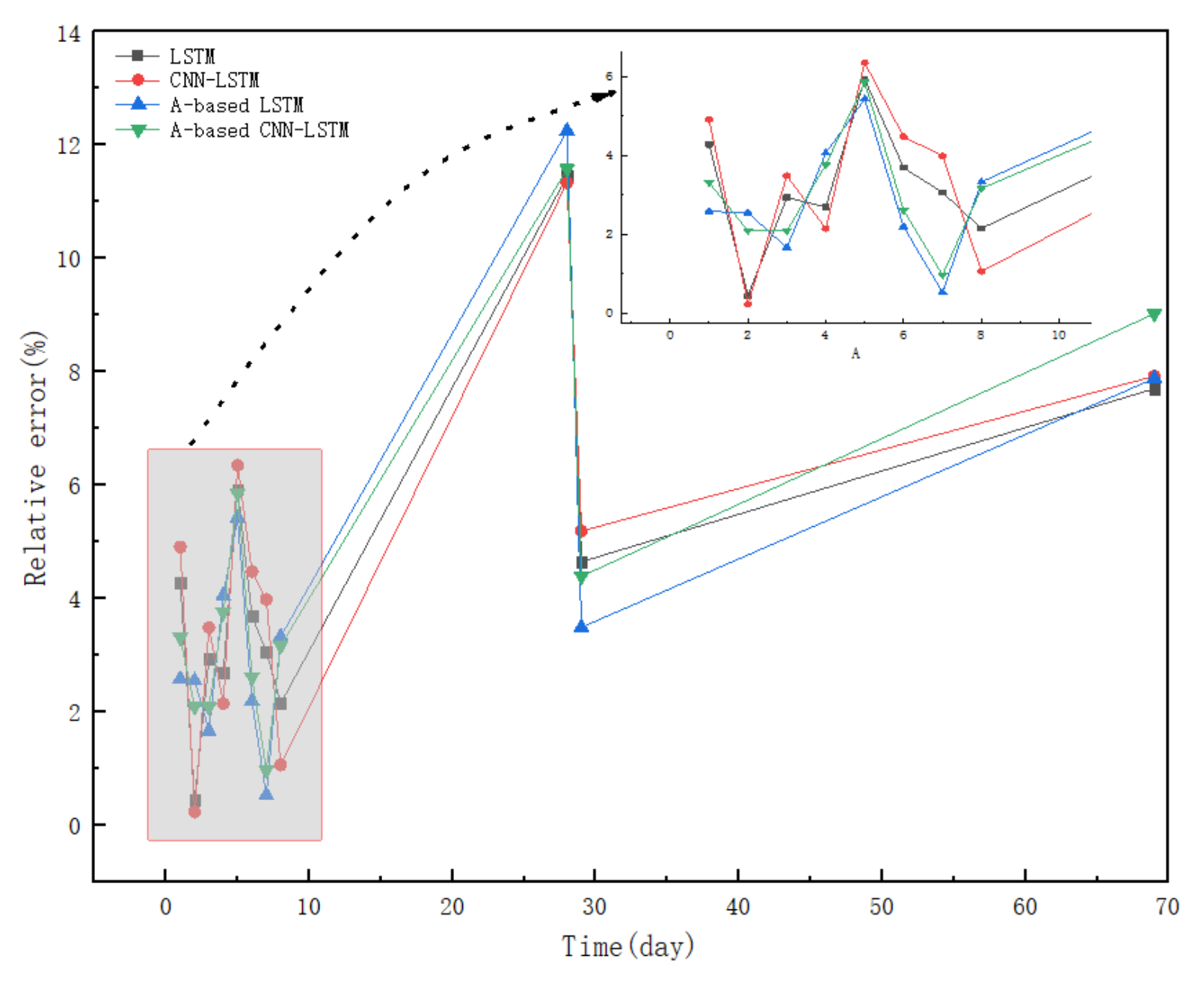
Analyzing the predicted values of these outliers for different models can evaluate the performance of these models. There are 11 outliers in the data of these 100 time points, which are water consumption on the 1st, 2nd, 3rd, 4th, 5th, 6th, 7th, 8th, 28th, 29th, and 69th days, respectively. Forecasting results of different models for outliers are shown in Figure 16. As can be seen from Figure 16, the attention-based LSTM model and attention CNN-LSTM hybrid model have good prediction effect on the continuous outliers in previous days, which are all less than the lower limit.
In order to accurately represent the prediction effect of each model on the outliers, the relative errors between these outliers and the predicted values of each model were calculated. Among the prediction results of outliers by different models, the MAPEs of the LSTM model, CNN-LSTM model, attention-based LSTM model, and attention-based CNN-LSTM hybrid model were 4.90%, 5.11%, 4.59% and 4.88% respectively. Figure 17 exhibits the relative errors between actual outliers and predicted values at each data point. It can be seen from Figure 17 that the relative error of these four models in predicting the abnormal water consumption on the 1st, 2nd, 3rd, 4th, 5th, 6th, 7th, and 8th days is less than 6%. However, the four models have the largest relative errors in predicting water consumption on the 28th day, which is more than 10%.
In order to show the prediction effect more accurately, six evaluation indexes are introduced to evaluate the four prediction models. Four evaluation indexes, MAE, RMSE, MAPE, and R2, are introduced to describe the improvement of the proposed method compared with the contract methods, and are shown in Table 5.

4.2. Discussions

In this paper, some classical deep learning models and methods, consisting of CNN model, LSTM model, encoder-decoder network, and AM, were integrated to improve the prediction accuracy of daily water demand. For verifying the superiorities of the attention-based CNN-LSTM hybrid model, LSTM model, CNN-LSTM model, and attention-based LSTM were selected as the comparison models to predict the daily water demand time series in Suzhou, China. The proposed model achieves higher prediction performance with the following four indices: MAE = 5773.90, RMSE = 7251.52, MAPE = 1.77%, and R2 = 0.924.
The four prediction models based on deep learning models and methods can anticipate the trend of real water demand (Figure 13). At the same time, the introduction of CNN model or AM is conducive to improving the performance of the prediction model in terms of six evaluation criterions (Table 5). Therefore, the attention-based CNN-LSTM hybrid model shows excellent performance compared with the contrast models that are applicable to time series forecasting. However, there are some differences in the performance of each model at each time point. As the structure of the model becomes more complex, the distribution of the predicted value of the model is more concentrated (Figure 12). It may be that the improvement of the learning ability of the model enables the forecast model to highlight the general distribution of actual water consumption. The prediction effect of the single LSTM model in some peaks values is better than other prediction models, which makes the overall prediction trend of the single LSTM model seem to be closer to the actual water demand (Figure 13a,c,e,g). Meanwhile, the correlation between the actual value and the predicted value of the LSTM model is the weakest (Figure 13b,d,f,h). The LSTM model is affected by some outliers due to the ability to learn the long-term nonlinear relationship of time series. Because the CNN model can remove the noise and unstable components from the data and take into consideration the correlation between multivariate variables, the introduction of the CNN model enhances the correlation between the predicted value and the actual value of the prediction models. Similarly, AM can underline the important time series characteristics and reduce the influence of some outliers on the prediction effect.
It is worth noting that the deep learning models with strong learning ability still have certain errors. As shown in Figure 17, the relative errors of the four models are mostly less than 6%, and their average relative errors are between 2% and 3%. According to the fact that the average relative error of outliers is larger than the overall average relative error of the load values in the 100 days, it can be concluded that these outliers have a certain impact on the prediction performance of the model. Moreover, the prediction accuracy of the four models for water consumption on the 28th and 69th days is relatively low, and the relative error of the two days is more than 6% (Figure 17). The water demand on the 28th day and the 29th day varies greatly compared with that on the latest day, which makes the models unable to accurately predict the load values of these two points. Since the variables of the latest day are used as input to the model, the four models that can learn the long-term nonlinear relationship also find it difficult to predict the very few rapidly changing load values.
Among the various water demand forecasting models, the proposed hybrid attention-based CNN-LSTM model has the characteristics of considering the correlation between multiple variables and ignoring irrelevant data points, which improves the prediction accuracy of the daily water demand and can provide measurement support for pumps scheduling in water supply system. Once the water supply data listed in Section 3.1 has been collected, the proposed model can be easily solved for real problems using optimization software. In addition, a system can be designed for decision-makers to display the forecast results in visualization with more advanced application.

5. Conclusions

Urban water demand prediction is beneficial for the design and optimal management of water distribution systems. Short-term water consumption prediction helps to identify appropriate options to maintain a balance between water supply and demand. In this paper, a hybrid framework called the attention-based CNN-LSTM model is proposed to predict daily water demand time series of the water plant in Suzhou, China. The proposed model is contrasted with the LSTM model, CNN-LSTM model, and attention-based LSTM, and the predicted load values of these models are consistent with the actual water demand. Among these models, the proposed model has better prediction performance in terms of MAE, RMSE, MAPE, and R2. The results show that the attention-based CNN-LSTM hybrid model not only has excellent performance in predicting daily water demand, but also has certain reference significance for the application of deep learning technology in time series forecasting.
A very small number of daily water consumption data rapidly change, which leads to the decline of the overall accuracy of the attention-based CNN-LSTM hybrid model for daily water demand forecasting. For the sake of working out this problem, several different statistical techniques should be applied to select a suitable model input with better forecast performance. In future work, with the development of deep learning technology, some new intelligent models and methods can be introduced to improve the prediction accuracy of fluctuating water demand data.

Author Contributions

Writing—original draft preparation, S.Z. and S.H.; writing—review and editing, B.D., J.G. and S.G.; visualization, J.G.; supervision, B.D. and S.G. All authors have read and agreed to the published version of the manuscript.

Funding

The National Natural Science Foundation of China (No. 51705386); China Scholarship Council (No.201606955091); Fundamental Research Funds for the Central Universities, China (No. 2018-IVB-010).

Institutional Review Board Statement

Not applicable.

Informed Consent Statement

Not applicable.

Data Availability Statement

Not applicable.

Acknowledgments

The authors are grateful for the valuable comments and suggestions by the respected reviewers, which enhanced the strength and significance of this work.

Conflicts of Interest

The authors declare no conflict of interest.

References

  1. Guo, W.; Liu, T.; Dai, F.; Xu, P. An improved whale optimization algorithm for forecasting water resources demand. Appl. Soft Comput. 2020, 86, 105925. [Google Scholar] [CrossRef]
  2. Niva, V.; Cai, J.; Taka, M.; Kummu, M.; Varis, O. China’s sustainable water-energy-food nexus by 2030: Impacts of urbanization on sectoral water demand. J. Clean. Prod. 2020, 251, 119755. [Google Scholar] [CrossRef]
  3. Niknam, A.; Zare, H.K.; Hosseininasab, H.; Mostafaeipour, A.; Herrera, M. A Critical Review of Short-Term Water Demand Forecasting Tools—What Method Should I Use? Sustainability 2022, 14, 5412. [Google Scholar] [CrossRef]
  4. Abdalla, G.; Özyurt, F. Sentiment Analysis of Fast Food Companies With Deep Learning Models. Comput. J. 2021, 64, 383–390. [Google Scholar] [CrossRef]
  5. Yalçıntaş, M.; Bulu, M.; Küçükvar, M.; Samadi, H. A framework for sustainable urban water management through demand and supply forecasting: The case of Istanbul. Sustainability 2015, 7, 11050–11067. [Google Scholar] [CrossRef]
  6. Haque, M.; Rahman, A.; Hagare, D.; Chowdhury, R.K. A Comparative Assessment of Variable Selection Methods in Urban Water Demand Forecasting. Water 2018, 10, 419. [Google Scholar] [CrossRef]
  7. Granata, F.; Papirio, S.; Esposito, G.; Gargano, R.; De Marinis, G. Machine Learning Algorithms for the Forecasting of Wastewater Quality Indicators. Water 2017, 9, 105. [Google Scholar] [CrossRef]
  8. Smolak, K.; Kasieczka, B.; Fialkiewicz, W.; Rohm, W.; Sila-Nowicka, K.; Kopanczyk, K. Applying human mobility and water consumption data for short-term water demand forecasting using classical and machine learning models. Urban Water J. 2020, 17, 32–42. [Google Scholar] [CrossRef]
  9. Koo, K.-M.; Han, K.-H.; Jun, K.-S.; Lee, G.; Kim, J.-S.; Yum, K.-T. Performance Assessment for Short-Term Water Demand Forecasting Models on Distinctive Water Uses in Korea. Sustainability 2021, 13, 6056. [Google Scholar] [CrossRef]
  10. Pesantez, J.E.; Berglund, E.Z.; Kaza, N. Smart meters data for modeling and forecasting water demand at the user-level. Environ. Model. Softw. 2020, 125, 104633. [Google Scholar] [CrossRef]
  11. Xu, Y.; Zhang, J.; Long, Z.; Lv, M. Daily Urban Water Demand Forecasting Based on Chaotic Theory and Continuous Deep Belief Neural Network. Neural Process. Lett. 2019, 50, 1173–1189. [Google Scholar] [CrossRef]
  12. Du, B.; Zhou, Q.; Guo, J.; Guo, S.; Wang, L. Deep learning with long short-term memory neural networks combining wavelet transform and principal component analysis for daily urban water demand forecasting. Expert Syst. Appl. 2021, 171, 114571. [Google Scholar] [CrossRef]
  13. Ebtehaj, I.; Bonakdari, H.; Gharabaghi, B. A reliable linear method for modeling lake level fluctuations. J. Hydrol. 2019, 570, 236–250. [Google Scholar] [CrossRef]
  14. Shen, Z.P.; Zhang, Y.M.; Lu, J.W.; Xu, J.; Xiao, G. A novel time series forecasting model with deep learning. Neurocomputing 2020, 396, 302–313. [Google Scholar] [CrossRef]
  15. Abbasimehr, H.; Shabani, M.; Yousefi, M. An optimized model using LSTM network for demand forecasting. Comput. Ind. Eng. 2020, 143, 13. [Google Scholar] [CrossRef]
  16. Hajiabotorabi, Z.; Kazemi, A.; Samavati, F.F.; Ghaini, F.M.M. Improving DWT-RNN model via B-spline wavelet multiresolution to forecast a high-frequency time series. Expert Syst. Appl. 2019, 138, 9. [Google Scholar] [CrossRef]
  17. Fekri, M.N.; Patel, H.; Grolinger, K.; Sharma, V. Deep learning for load forecasting with smart meter data: Online Adaptive Recurrent Neural Network. Appl. Energy 2020, 282, 116177. [Google Scholar] [CrossRef]
  18. Sagheer, A.; Kotb, M. Time series forecasting of petroleum production using deep LSTM recurrent networks. Neurocomputing 2019, 323, 203–213. [Google Scholar] [CrossRef]
  19. Liu, Y. Novel volatility forecasting using deep learning-Long Short Term Memory Recurrent Neural Networks. Expert Syst. Appl. 2019, 132, 99–109. [Google Scholar] [CrossRef]
  20. Abdel-Nasser, M.; Mahmoud, K. Accurate photovoltaic power forecasting models using deep LSTM-RNN. Neural Comput. Appl. 2019, 31, 2727–2740. [Google Scholar] [CrossRef]
  21. Yu, Y.; Hu, C.H.; Si, X.S.; Zheng, J.F.; Zhang, J.X. Averaged Bi-LSTM networks for RUL prognostics with non-life-cycle labeled dataset. Neurocomputing 2020, 402, 134–147. [Google Scholar] [CrossRef]
  22. Bouktif, S.; Fiaz, A.; Ouni, A.; Serhani, M.A. Multi-Sequence LSTM-RNN Deep Learning and Metaheuristics for Electric Load Forecasting. Energies 2020, 13, 391. [Google Scholar] [CrossRef]
  23. Shahid, F.; Zameer, A.; Muneeb, M. Predictions for COVID-19 with deep learning models of LSTM, GRU and Bi-LSTM. Chaos Solitons Fractals 2020, 140, 110212. [Google Scholar] [CrossRef] [PubMed]
  24. Kim, T.-Y.; Cho, S.-B. Predicting residential energy consumption using CNN-LSTM neural networks. Energy 2019, 182, 72–81. [Google Scholar] [CrossRef]
  25. Wang, K.; Li, K.L.; Zhou, L.Q.; Hu, Y.K.; Cheng, Z.Y.; Liu, J.; Chen, C. Multiple convolutional neural networks for multivariate time series prediction. Neurocomputing 2019, 360, 107–119. [Google Scholar] [CrossRef]
  26. Khaki, S.; Wang, L.; Archontoulis, S.V. A CNN-RNN Framework for Crop Yield Prediction. Front. Plant Sci. 2020, 10, 1750. [Google Scholar] [CrossRef] [PubMed]
  27. Li, T.Y.; Hua, M.; Wu, X. A Hybrid CNN-LSTM Model for Forecasting Particulate Matter (PM2.5). IEEE Access 2020, 8, 26933–26940. [Google Scholar] [CrossRef]
  28. Essien, A.; Giannetti, C. A Deep Learning Model for Smart Manufacturing Using Convolutional LSTM Neural Network Autoencoders. IEEE Trans. Industr. Inform. 2020, 16, 6069–6078. [Google Scholar] [CrossRef]
  29. Taieb, S.B.; Atiya, A.F. A Bias and Variance Analysis for Multistep-Ahead Time Series Forecasting. IEEE Trans. Neural Networks Learn. Syst. 2016, 27, 62–76. [Google Scholar] [CrossRef]
  30. Xiao, Y.; Yin, H.; Zhang, Y.; Qi, H.; Zhang, Y.; Liu, Z. A dual-stage attention-based Conv-LSTM network for spatio-temporal correlation and multivariate time series prediction. Int. J. Intell. Syst. 2021, 36, 2036–2057. [Google Scholar] [CrossRef]
  31. Du, S.; Li, T.; Yang, Y.; Horng, S.-J. Multivariate time series forecasting via attention-based encoder-decoder framework. Neurocomputing 2020, 388, 269–279. [Google Scholar] [CrossRef]
  32. Liu, Q.; Wang, B.; Zhu, Y. Short-Term Traffic Speed Forecasting Based on Attention Convolutional Neural Network for Arterials. Comput. Civ. Infrastruct. Eng. 2018, 33, 999–1016. [Google Scholar] [CrossRef]
  33. Ding, Y.; Zhu, Y.; Feng, J.; Zhang, P.; Cheng, Z. Interpretable spatio-temporal attention LSTM model for flood forecasting. Neurocomputing 2020, 403, 348–359. [Google Scholar] [CrossRef]
  34. Liu, Y.; Gong, C.; Yang, L.; Chen, Y. DSTP-RNN: A dual-stage two-phase attention-based recurrent neural network for long-term and multivariate time series prediction. Expert Syst. Appl. 2020, 143, 113082. [Google Scholar] [CrossRef]
  35. Wang, S.; Wang, X.; Wang, S.; Wang, D. Bi-directional long short-term memory method based on attention mechanism and rolling update for short-term load forecasting. Int. J. Electr. Power Energy Syst. 2019, 109, 470–479. [Google Scholar] [CrossRef]
  36. Li, Y.; Zou, L.; Jiang, L.; Zhou, X. Fault Diagnosis of Rotating Machinery Based on Combination of Deep Belief Network and One-dimensional Convolutional Neural Network. IEEE Access 2019, 7, 165710–165723. [Google Scholar] [CrossRef]
  37. Fang, X.; Yuan, Z. Performance enhancing techniques for deep learning models in time series forecasting. Eng. Appl. Artif. Intell. 2019, 85, 533–542. [Google Scholar] [CrossRef]
  38. Yang, S.; Yang, D.; Chen, J.; Zhao, B. Real-time reservoir operation using recurrent neural networks and inflow forecast from a distributed hydrological model. J. Hydrol. 2019, 579, 124229. [Google Scholar] [CrossRef]
  39. Kao, I.F.; Zhou, Y.; Chang, L.-C.; Chang, F.-J. Exploring a Long Short-Term Memory based Encoder-Decoder framework for multi-step-ahead flood forecasting. J. Hydrol. 2020, 583, 124631. [Google Scholar] [CrossRef]
  40. Zubaidi, S.L.; Gharghan, S.K.; Dooley, J.; Alkhaddar, R.M.; Abdellatif, M. Short-Term Urban Water Demand Prediction Considering Weather Factors. Water Resour. Manag. 2018, 32, 4527–4542. [Google Scholar] [CrossRef]
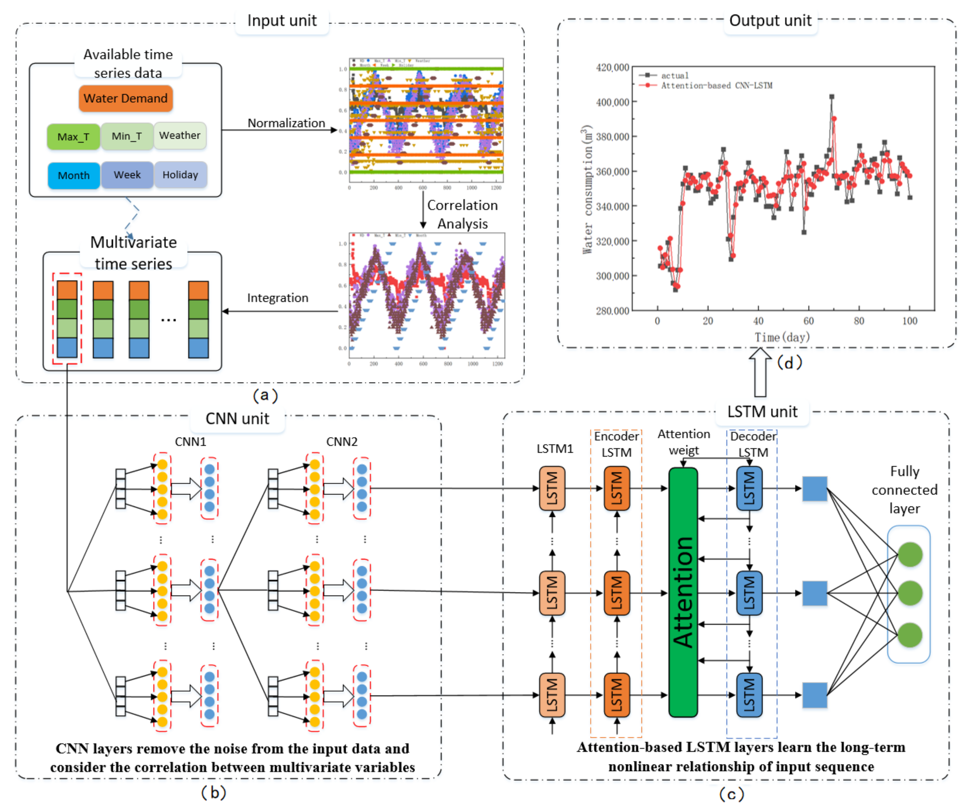
Figure 1. The overall architecture of the attention-based CNN-LSTM hybrid model, (a) Input unit, (b) CNN unit, (c) LSTM unit and (d) Output unit.
Sustainability 14 11086 g001
Figure 2. The process of 1D-CNN dealing with a multivariate time series.
Sustainability 14 11086 g002
Figure 3. The internal structure of a single LSTM cell.
Sustainability 14 11086 g003
Figure 4. The structure of the encoder-decoder network based on deep LSTM networks.
Sustainability 14 11086 g004
Figure 5. The architecture of the attention-based deep LSTM model.
Sustainability 14 11086 g005
Figure 6. The water plant location map of the case study.
Sustainability 14 11086 g006
Figure 7. The box plot of water demand in 2016, 2017, 2018, 2019, holiday, and weekday.
Sustainability 14 11086 g007
Figure 8. (a) The average daily water consumption of each month in 2016, 2017, 2018, and 2019. (b) Water demand, Max-T, and Min-T for August 2016.
Sustainability 14 11086 g008
Figure 9. The plots of water demand time series for total, training, validation, and testing period alongside statistical characteristic charts. (a,b) are diagram and box plots for training, validation and testing sets, (cf) are frequency histogram of total, training, validation and testing water demand.
Sustainability 14 11086 g009
Figure 10. Training history of different models.
Sustainability 14 11086 g010
Figure 11. Water consumption forecasting results of models.
Sustainability 14 11086 g011
Figure 12. The box plots of actual values and predictive values for different models.
Sustainability 14 11086 g012
Figure 13. Forecasting results and scatter plots of the four models. Panels (a,b) are the LSTM model, (c,d) are the CNN-LSTM model, (e,f) are the attention-based LSTM model, and (g,h) are the attention-based CNN-LSTM model.
Sustainability 14 11086 g013aSustainability 14 11086 g013b
Figure 14. Relative errors distribution of each model.
Sustainability 14 11086 g014
Figure 15. The distribution of these outliers. Panel (a) is the box plot of the actual 100 days water consumption, (b) is the distribution of outliers in red dots.
Sustainability 14 11086 g015
Figure 16. Forecasting results of different models for outliers, (a) LSTM model, (b) CNN-LSTM model, (c) attention-based LSTM model and (d) attention-based CNN-LSTM model.
Sustainability 14 11086 g016
Figure 17. Relative errors of outliers in each model.
Sustainability 14 11086 g017
Table 1. Summary of historical daily data.
Historical DataFeatureCharacterization
Consumption dataL(d − 1), L(d − 2), …, L(d − n)Historical water demand series in the previous n days
Meteorological dataMax-TDaily maximum temperature
Min-TDaily minimum temperature
W-dataEncode weather with different weather types according to local weather forecast, such as cloudy, rainy, sunny, snowy, windy, foggy days, etc.
Date dataM-label1 to 12 represent January to December, respectively
W-label1 to 7 denote Monday to Sunday, respectively
H-label1 label holidays, 0 label work days
Table 2. Pearson correlation coefficient of water consumption in different days.
ConsumptionL(d)L(d − 1)L(d − 2)L(d − 3)L(d − 4)L(d − 5)L(d − 6)
L(d)10.920 **0.879 **0.857 **0.831 **0.802 **0.782 **
L(d − 1)0.920 **10.920 **0.879 **0.857 **0.831 **0.802 **
L(d − 2)0.879 **0.920 **10.920 **0.879 **0.857 **0.831 **
L(d − 3)0.857 **0.879 **0.920 **10.920 **0.879 **0.857 **
L(d − 4)0.831 **0.857 **0.879 **0.920 **10.920 **0.879 **
L(d − 5)0.802 **0.831 **0.857 **0.879 **0.920 **10.920 **
L(d − 6)0.782 **0.802 **0.831 **0.857 **0.879 **0.920 **1
** Correlation is significant at the 0.01 level (two-tailed).
Table 3. Spearman correlation coefficient of collected influential factors data.
FactorsLMax-TMin-TW-DataM-labelW-LabelH-Label
L1.0000.473 **0.444 **−0.0250.395 **0.020−0.031
Max-T0.473 **1.0000.963 **0.0070.335 **0.000−0.022
Min-T0.444 **0.963 **1.0000.0340.358 **−0.005−0.024
W-data−0.0250.0070.0341.000−0.0070.0160.013
M-label0.395 **0.335 **0.358 **−0.0071.0000.003−0.026
W-label0.0200.000−0.0050.0160.0031.0000.686 **
H-label−0.031−0.022−0.0240.013−0.0260.686 **1.000
** Correlation is significant at the 0.01 level (two-tailed).
Table 4. Main structure of different predictive network models.
ModelBatch SizeLearning RateEpochsLayersHidden Layers Size
LSTM200.0022004LSTM (48,16)
CNN-LSTM200.0011606CNN (6,3), LSTM (24,4)
A-based LSTM300.0013007LSTM (24,24), AM (24)
A-based CNN-LSTM300.0012508CNN (6,3), LSTM (24,24,24), AM (24)
Table 5. Performance evaluations of different models.
ModelsMAE/m3RMSE/m3MAPE/%R2
LSTM7528.9510,074.992.340.854
CNN-LSTM6550.089131.562.030.880
Attention-based LSTM6269.188727.571.940.890
Attention-based CNN-LSTM5773.907251.521.770.924
Publisher’s Note: MDPI stays neutral with regard to jurisdictional claims in published maps and institutional affiliations.