Techno-Economic Comprehensive Review of State-of-the-Art Geothermal and Solar Roadway Energy Systems

Abstract

Road infrastructure is a vital constituent element in the transportation network; however, roadway surface ice and snow accumulation leads to huge traffic accidents in winter. Geothermal roadway energy systems (GRES) and solar roadway energy systems (SRES) can increase or decrease roadway surface temperature for the de-icing and removal of snow in winter, or mitigation of heat in summer. Technology performance and economic evaluation of the GRES and SRES are reviewed in this paper based on numerical and economic models, and experimental analyses. Three crucial aspects of the technology performance assessment, i.e., roadway surface temperature, energy consumption and key factors, are explored in different regions and countries. Economic evaluation approaches for net present values and payback periods of the GRES and SRES are investigated. The recommendations and potential future developments on the two technologies are deliberated; it is demonstrated that the GRES and SRES could increase roadway surface temperature by around 5 °C in winter and decrease it by about 6 °C in summer, with the payback periods of 4 to 8 years and 2.3 to 5 years, respectively.

1. Introduction

The roadway and bridge are the primary civil infrastructures used to link different regions [1], and are considered the structure platforms; however, the bridge decks and roadway surfaces are exposed to solar radiation and vehicle loading, which causes thermal gradient and mechanical vibration within the layers of the pavement [2,3]. Additionally, freezing and snow accumulation damage the roadway and compromise road user safety [4,5]. The conventional way for de-icing and snow melting roadway is to utilize salts (i.e., calcium chloride, sodium chloride and potassium acetate) and other chemical materials, which is able to bring down the freezing point of water to avert the formation of ice [6,7]. Nevertheless, this approach raises some issues and has some limitations, such as soil pollution, vehicle corrosion, declined durability of pavement material, temperature limitation (below −3.9 °C), large manpower and being dangerous to the environment [8,9]. Hence, some alternative methods to remove snow and ice are exploited to avoid the above issues. By far, two renewable energy technologies, geothermal roadway energy system (GRES) and solar roadway energy system (SRES), are becoming promising for snow melting and de-icing applications due to their cost-effective and pro-environment characteristics [10,11]. Specifically, the GRES extracts heat from geothermal hot water and soil; meanwhile, it is able to absorb solar energy during sunny days and releases heat for ice and snow melting in winter. In summer, the system could cool the roadway, store heat within the soil for being reused in winter [12,13]. On the other hand, the utilization of solar energy largely involves two modes: converting solar radiation into heat and electricity energy. The heat can be utilized to melt snow and ice on roadways in winter, while the electricity could be supplied to the grid, or utilized for unmanned driving of smart roads and wireless charging in the future [14,15].

Conventionally, de-icing and removal of snow on road surfaces is done based on an integrated manual and machine-based solution which are expensive as well; however, this method to monitor damage is not just a waste of time but is also ineffective since the detection of such damages needs consistent assist from subject matter experts who have the ability to identify and differentiate various categories of pavement failures. Thereby, in this review, the renewable energy technology is employed to get command of the roadway surface temperature owing to the de-icing and removal of snow in winter, or mitigation of heat in summer; these designated and retrieved cited studies are concerning the techno-economic analysis of the GRES and SRES applied in various countries and areas, and the numerical models and experimental test are performed based on different boundaries and assumption conditions including weather condition, fluid velocity, solar radiation, initial temperature, thermal properties definitions and economic index. For the current research, the most challenging point in designing the GRES and SRES is to identify heat source. Although the two technologies are taken into account as alternative solutions, their performance and costs are influenced by climatic conditions, working fluid, pipe configuration, soil property, concrete slab and initial conditions. Hence, the aim of this study is to review the techno-economic performance of the GRES and SRES applied in roadways to provide comprehensive information regarding numerical models, experimental data and advancement of engineering application. Firstly, the basic knowledge of the two systems is described in Section 2, then, the technical analyses, for example, numerical modeling, laboratory research, field testing and material design, are summarized in Section 3. The economic assessment of the two systems is clarified in Section 4, whereas the future challenges and recommendations are put forward in Section 5, the key conclusions are presented in Section 6.

2. Geothermal and Solar Roadway Energy Systems

Figure 1 depicts the effective energy-extracted technologies that could be utilized in the road. By far, the GRES and SRES are becoming promising and advanced solutions for snow melting and de-icing applications.

2.1. Geothermal Roadway Energy System

The GRES is a renewable-based energy system applied on a roadway. There are two core sections of the system, de-icing (and/or heating) roadway by soil heat energy extracted in winter and cooling roadway via circulated working fluid in summer. Normally, a GRES consists of a ground heat exchanger, a pipe network and a heat pump. Figure 2 presents a detailed illustration of the working principle of a GRES [5,16,17]. In winter, the stored heat is released to the roadway surface for de-icing and snow melting. While in summer, the roadway surface exposed to the sun reaches a high temperature ranging between 60 °C and 70 °C [18,19], so this thermal energy can be stored. The working fluid is circulated to cool warm pavement with the aim of decreasing roadway surface temperature. Subsequently, the working fluid is circulated back to the ground, which acts as a heat energy storage, for utilization during the heating season [20,21]. Generally, traditional GRES needs a set number of buried pipe heat exchangers which are independent of the foundation structure. In order to overcome the drawback, a bi-functional GRES, called an energy pile (EP) system, is utilized to support loads of structure and exchange heat with soil to reduce the initial cost of installation; furthermore, various types of pipe such as single U-tube, double U-tube, tripe U-tube and helical pipe have been used in the GRES, which are utilized to test and compare system performance.

2.2. Solar Roadway Energy System

The SRES is another renewable technology-based system applied on the roadway. Typically, an SRES comprises a pipe network with a working fluid inside, buried beneath a roadway. When the roadway absorbs energy from the sun, its temperature is raised and the heat is transferred to a working fluid within the pipe network because of temperature difference. As depicted in Figure 3, there are three fundamental heat transfer processes in the SRES including convection, conduction and radiation [6,22,23]. In the conduction process, heat is conducted between the pipe walls and the roadway; this heat convection takes place when there are temperature gradients among the roadway, pipe walls and the thermal fluid. The radiation process happens through electromagnetic waves without any material medium, whereby the solar radiations are transmitted to the roadway whereas heat is radiated between the roadway and air temperature [3,24]. Generally, an SRES has the ability to alleviate the influence of the heat island effect (HIE) by means of decreasing roadway temperature [25]. The cooling effect contributes to sustaining roadway performance as well as reducing roadway deterioration under high-temperature climate conditions.

3. Technical Evaluation

3.1. Geothermal Roadway Energy System

The GRES has the advantages of using renewable energy sources and is environmentally friendly, improved roadway service life, and decreased urban HIE [25,26]. The effects of using different pipe arrangements for de-icing and snow melting are summarized in the subsequent sections.

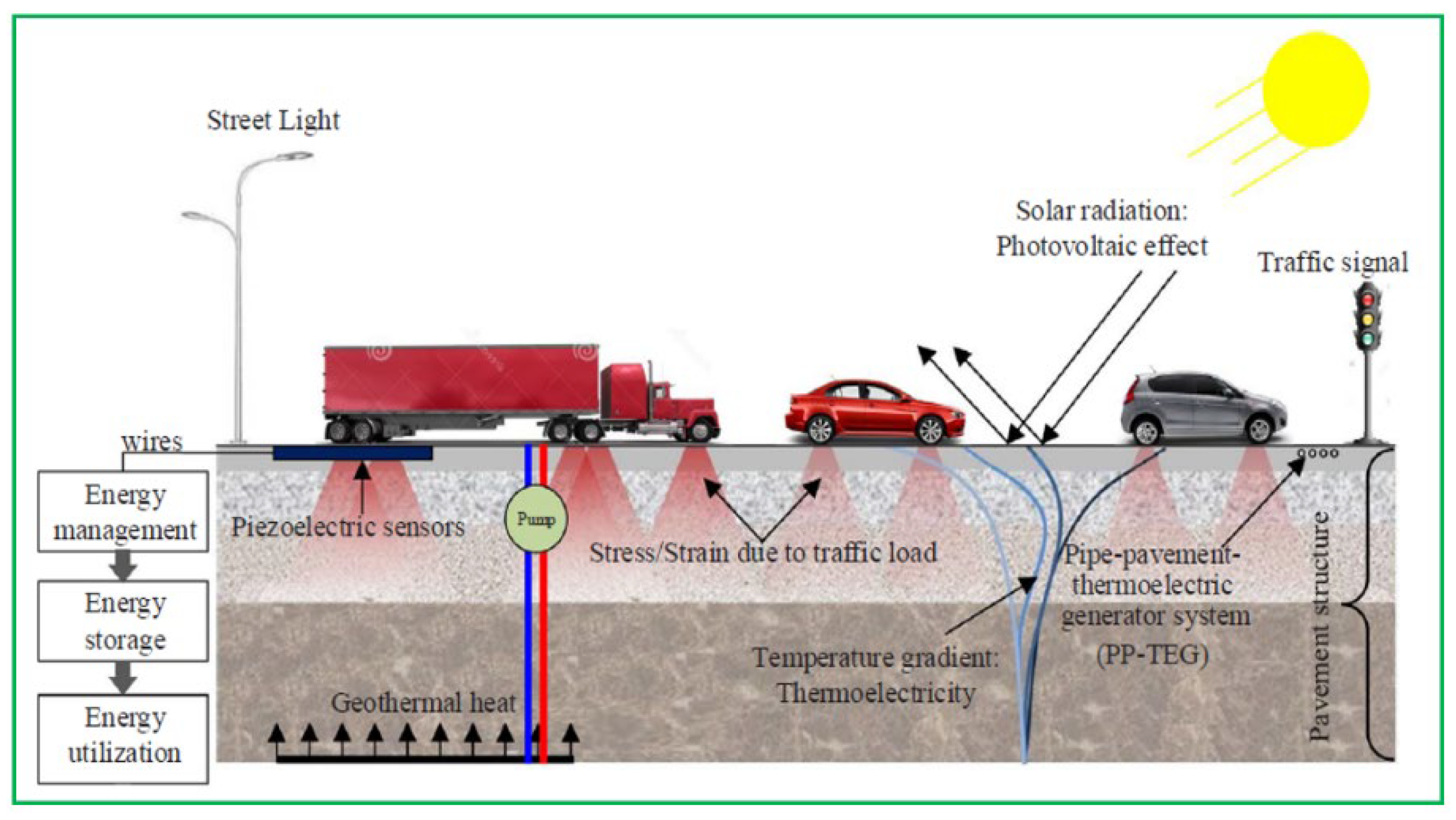
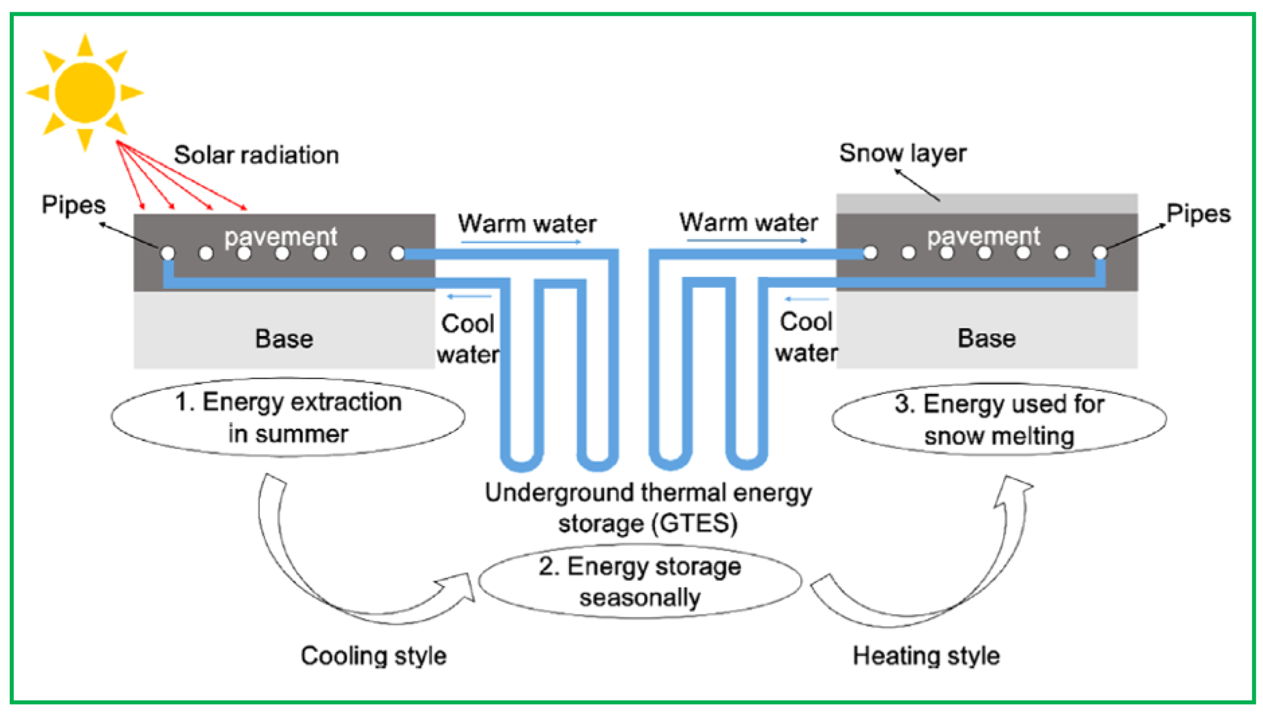
3.1.1. Geothermal Bridge Deck Energy System

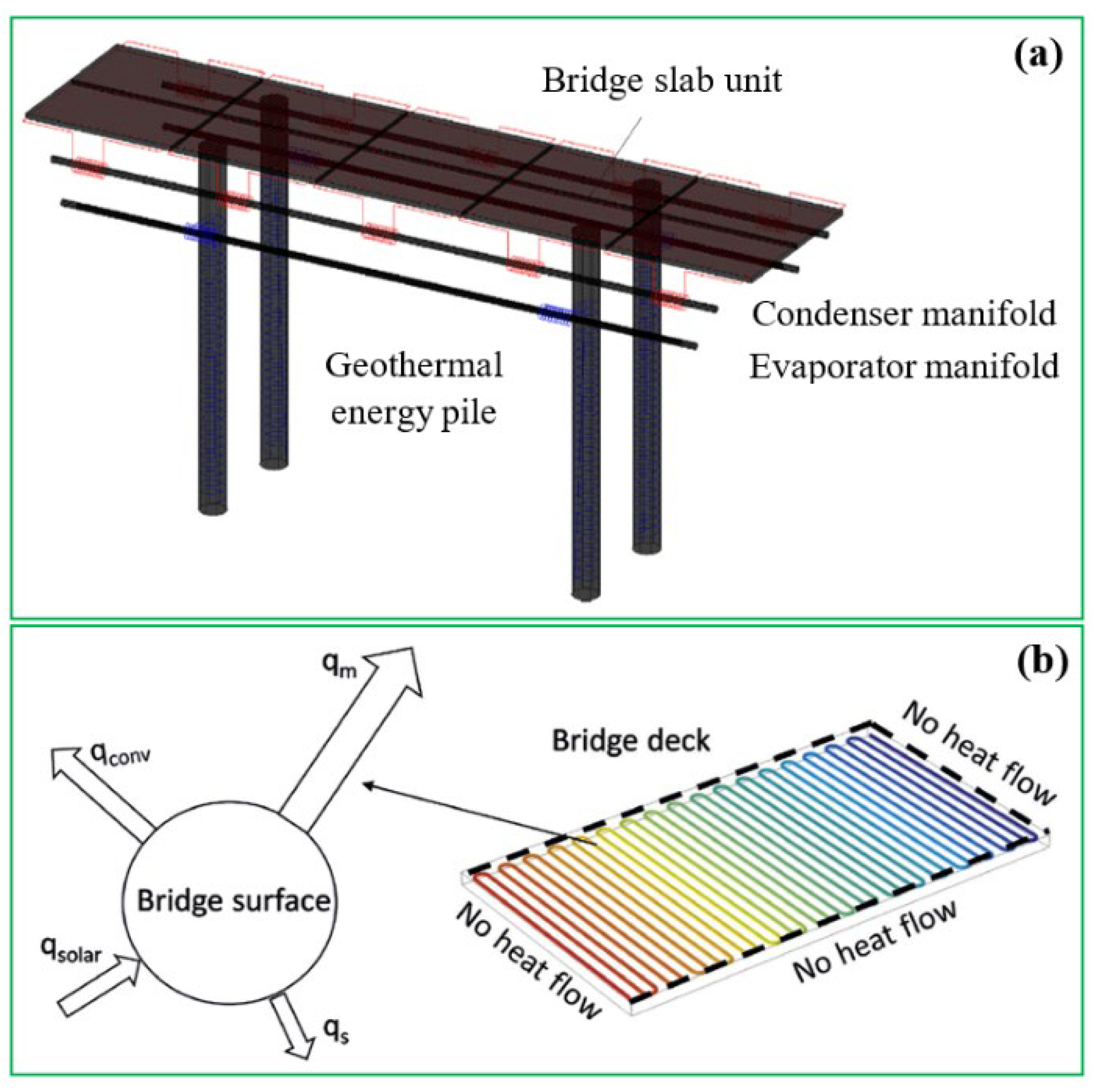
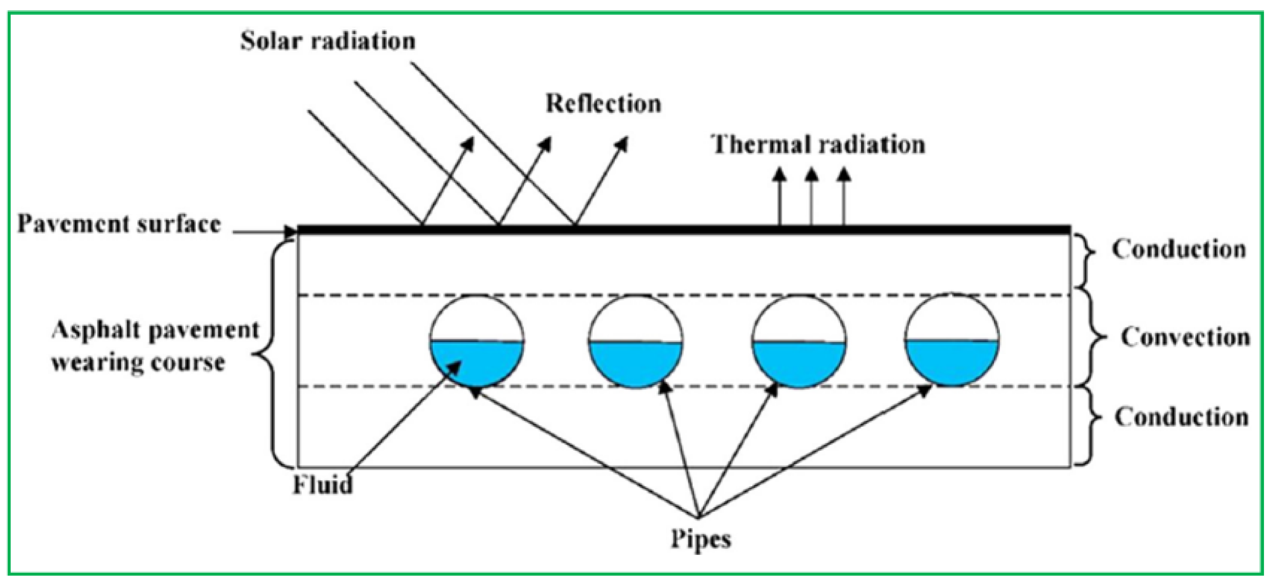
Liu et al. [26,27] developed a transient heat transfer model of the GRES for bridge deck to assess the influences of climate conditions and flow rate on system performance in Canada. Figure 4a presents the GRES based on the EP solution. Figure 4b illustrates the heat transfer mechanism of the bridge deck on the basis of radiation, convection as well as sensible and latent heat.

Table 1. Energy balance equation [26].

Description	Equations
Energy balance	$\mathrm{q}={\mathrm{q}}_{\mathrm{c}\mathrm{o}\mathrm{n}\mathrm{v}}+{\mathrm{q}}_{\mathrm{s}}+{\mathrm{q}}_{\mathrm{m}}+{\mathrm{q}}_{\mathrm{s}\mathrm{o}\mathrm{l}\mathrm{a}\mathrm{r}}$ ${\mathrm{q}}_{\mathrm{c}\mathrm{o}\mathrm{n}\mathrm{v}}(\mathrm{t})={\mathrm{h}}_{\mathrm{c}\mathrm{o}\mathrm{n}\mathrm{v}}[{\mathrm{T}}_{\mathrm{a}}(\mathrm{t})-{\mathrm{T}}_{\mathrm{s}}(\mathrm{t})]$ ${\mathrm{q}}_{\mathrm{m}}(\mathrm{t})={\mathsf{\rho }}_{\mathrm{w}}\mathrm{s}(\mathrm{t}){\mathrm{h}}_{\mathrm{f}}$ ${\mathrm{q}}_{\mathrm{s}}(\mathrm{t})={\mathsf{\rho }}_{\mathrm{w}}\mathrm{s}(\mathrm{t})[{\mathrm{c}}_{\mathsf{\rho }}^{\mathrm{i}}({\mathrm{T}}_{\mathrm{m}}-{\mathrm{T}}_{\mathrm{a}}(\mathrm{t})+{\mathrm{c}}_{\mathsf{\rho }}^{\mathrm{w}}({\mathrm{T}}_{\mathrm{f}}-{\mathrm{T}}_{\mathrm{m}})]$
Heat transfer within the working fluid	${\mathsf{\rho }}_{\mathrm{w}}{\mathrm{A}}_{\mathrm{g}\mathrm{f}}{\mathrm{C}}_{\mathrm{p}\mathrm{w}}\frac{\partial {\mathrm{T}}_{\mathrm{g}\mathrm{f}}}{\partial \mathrm{t}}+{\mathsf{\rho }}_{\mathrm{w}}{\mathrm{A}}_{\mathrm{g}\mathrm{f}}{\mathrm{C}}_{\mathsf{\rho }\mathrm{w}\mathrm{v}\mathrm{g}}\nabla {\mathrm{T}}_{\mathrm{g}\mathrm{f}}=\nabla \cdot ({\mathrm{A}}_{\mathrm{g}\mathrm{f}}{\mathrm{k}}_{\mathrm{w}}\nabla {\mathrm{T}}_{\mathrm{g}\mathrm{f}})+{\mathrm{Q}}_{\mathrm{w}2}$
Temperature distribution within the pipe	$\mathsf{\eta }=\frac{\mathrm{P}{\mathrm{V}}_{\mathrm{o}\mathrm{u}\mathrm{t}\mathrm{p}\mathrm{u}\mathrm{t}}}{\mathrm{A}\times \mathrm{I}}$ ${\mathsf{\rho }}_{\mathrm{w}}{\mathrm{A}}_{\mathrm{h}\mathrm{f}}{\mathrm{C}}_{\mathrm{p}\mathrm{w}}\frac{\partial {\mathrm{T}}_{\mathrm{h}\mathrm{f}}}{\partial \mathrm{t}}+{\mathsf{\rho }}_{\mathrm{w}}{\mathrm{A}}_{\mathrm{h}\mathrm{f}}{\mathrm{C}}_{\mathrm{p}\mathrm{v}\mathrm{s}}\nabla {\mathrm{T}}_{\mathrm{h}\mathrm{f}}=\nabla \cdot ({\mathrm{A}}_{\mathrm{h}\mathrm{f}}{\mathrm{k}}_{\mathrm{w}}\nabla {\mathrm{T}}_{\mathrm{h}\mathrm{f}})+{\mathrm{Q}}_{\mathrm{w}1}$ ${\mathrm{Q}}_{\mathrm{w}1}={(\mathrm{h}\mathrm{Z})}_{\mathrm{e}\mathrm{f}\mathrm{f}}({\mathrm{T}}_{\mathrm{e}\mathrm{x}\mathrm{t}}-\mathrm{T})$
Heat transfer around concrete slab	${\mathsf{\rho }}_{\mathrm{s}}{\mathrm{A}}_{\mathrm{c}\mathrm{s}}{\mathrm{C}}_{{}_{\mathrm{p}}}^{\mathrm{s}}\frac{\partial {\mathrm{T}}_{\mathrm{c}\mathrm{s}}}{\partial \mathrm{t}}=\nabla \cdot ({\mathrm{A}}_{\mathrm{c}\mathrm{s}}{\mathrm{k}}_{\mathrm{s}}\nabla \mathrm{T})-{\mathrm{Q}}_{\mathrm{w}1}$
Heat transfer within the soil	$\mathsf{\rho }\mathrm{A}{\mathrm{C}}_{\mathrm{p}}\frac{\partial {\mathrm{T}}_{\mathrm{s}}}{\partial \mathrm{t}}=\nabla \cdot (\mathrm{A}\mathrm{k}\nabla {\mathrm{T}}_{\mathrm{s}})-{\mathrm{Q}}_{\mathrm{w}2}$

exhibits the energy balance equations.

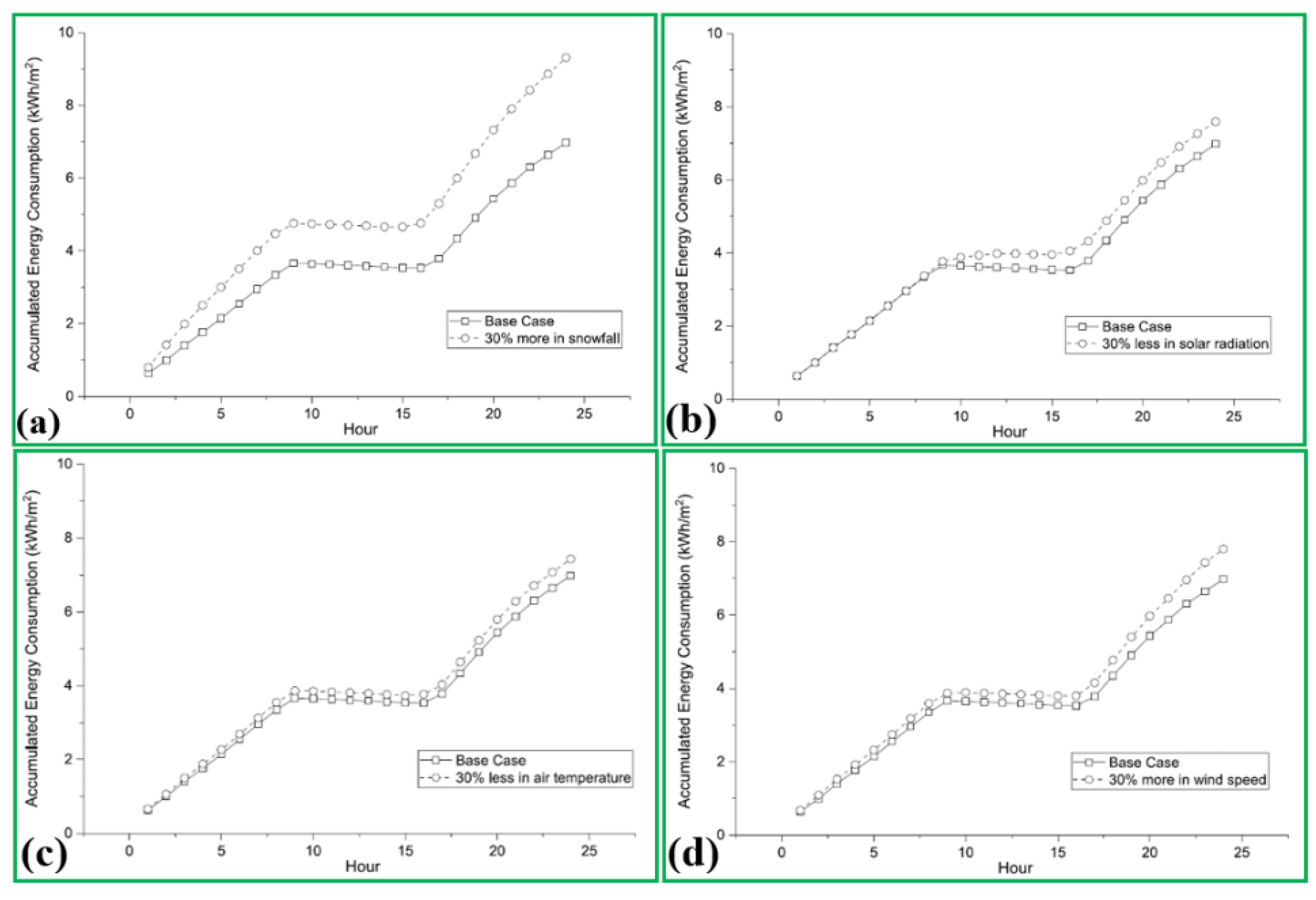
Figure 5 shows the effects of various influence factors, including snowfall rate, solar radiation, ambient temperature and wind speed, on energy consumption. Results reveal that the increases in snowfall rate and wind speed could give rise to a growth in energy consumption of 35% and 12% whereas the decreases in solar radiation and air temperature could increase energy consumption by 9% and 6.4%, respectively.

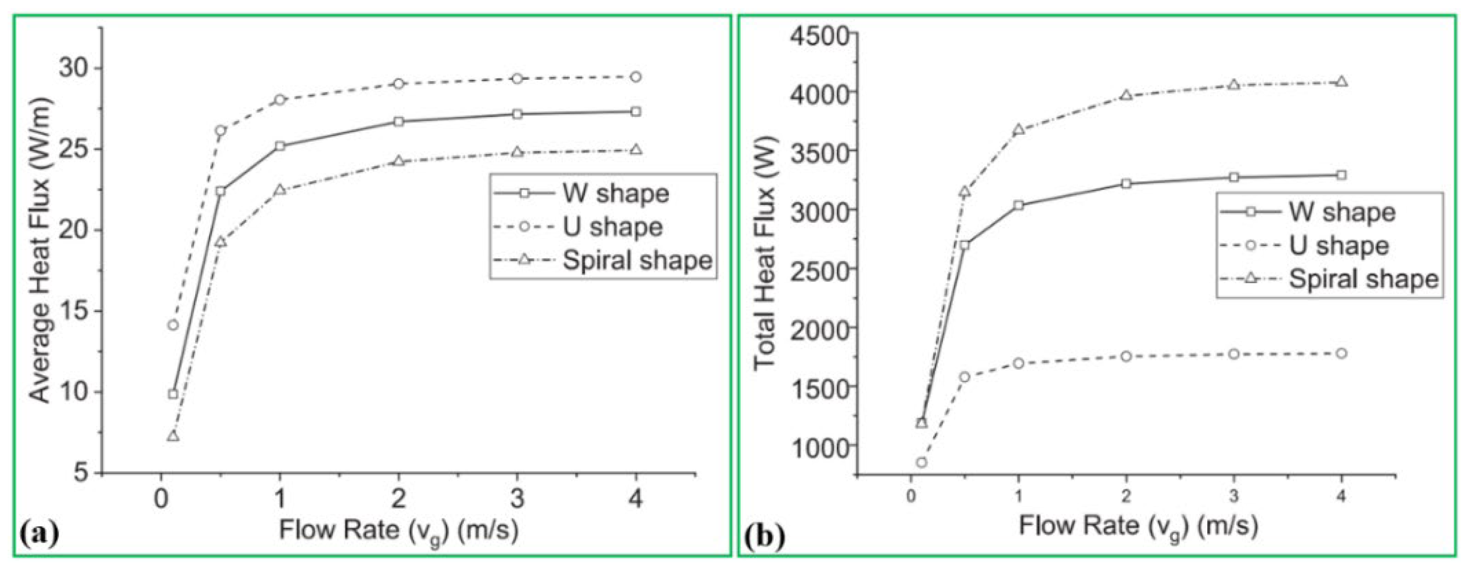
As demonstrated in Figure 6, the heat extraction rate of the GRES in terms of spiral-, W- and U- shapes could be enhanced by 3.4, 2.7 and 2 times, respectively, when the flow rates vary from 0.1 m/s to 4 m/s; this implies that the flow rate has the most vital influence on the heat extraction rate of the spiral shape.

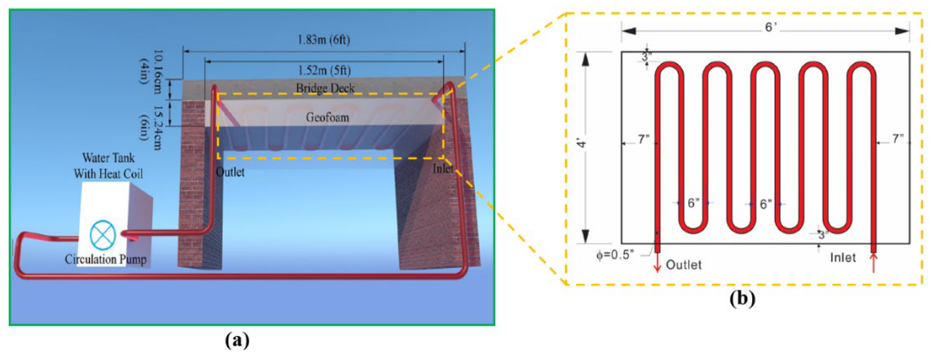
Yu et al. [28] designed an experimental rig of the GRES to investigate heat transfer characteristic and renovate some existing bridges. The schematic diagrams of the GRES and polyethylene pipe loop are exhibited in Figure 7. A lab-scale testing is performed to estimate temperature variation of the concrete slab at different locations as presented in Figure 8; this system consists of 10 polyethylene pipes with a diameter of 13 mm, a water tank and a pump. In the testing, the indoor and water tank temperatures are setup to 4.4 °C and 32.2 °C, respectively. 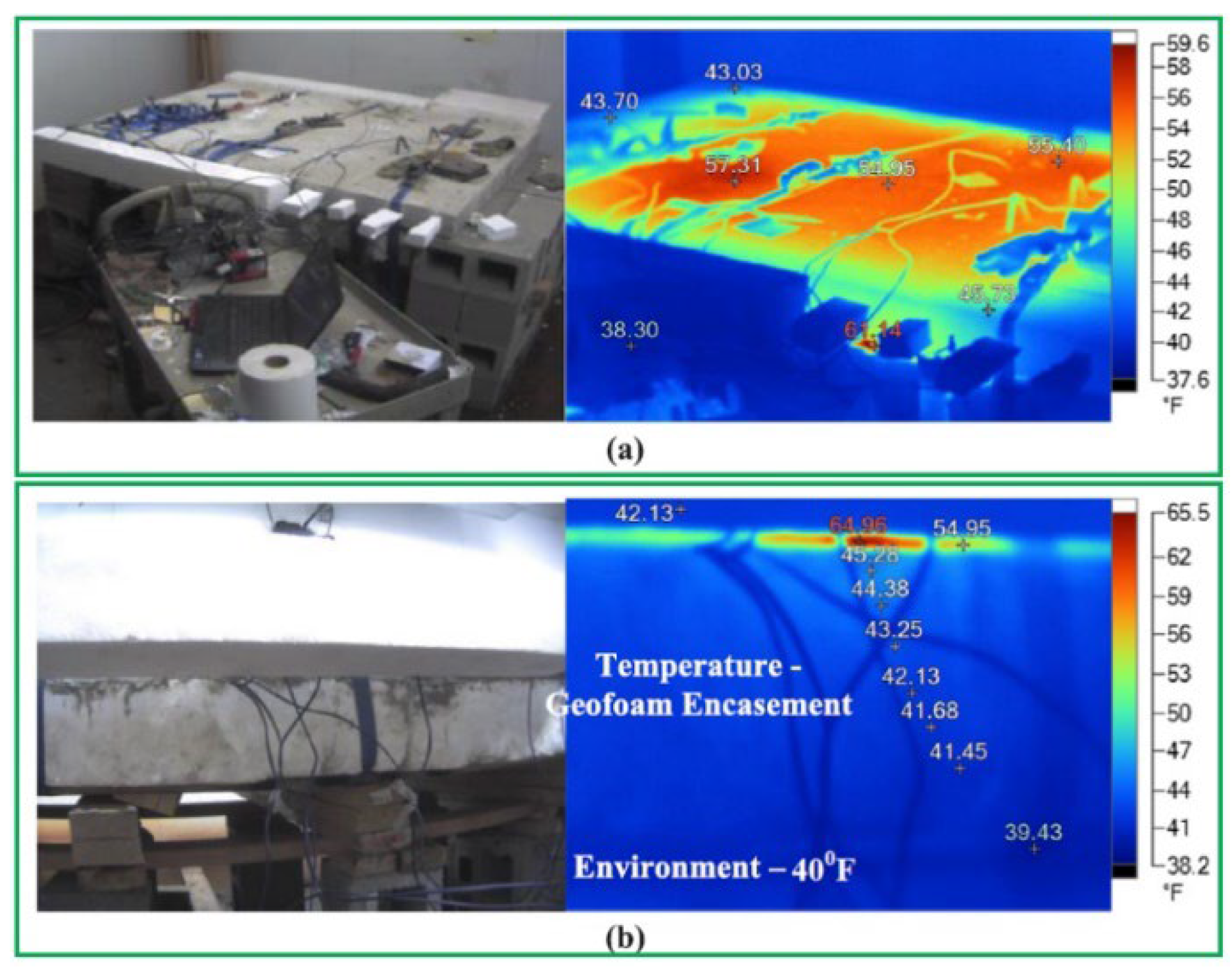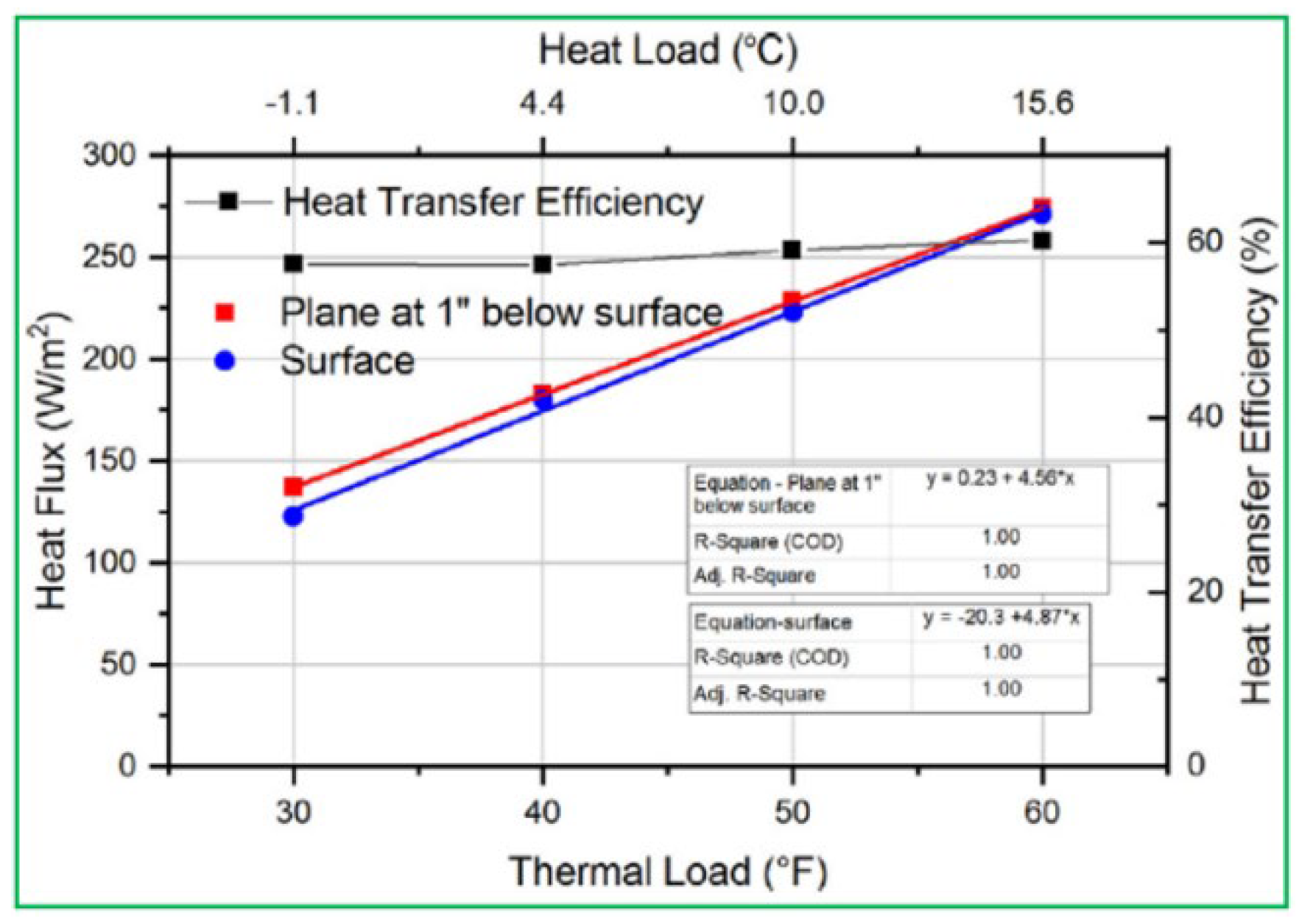Figure 9 displays the infrared pictures of the temperature distribution on the slab surface, which could reach an average of 12.8 °C (55 °F); it is indicated that the temperature is higher towards the centre of the concrete slab and progressively reduces outwards. In comparison, the mean temperature at the interface of the geofoam and concrete is 16.1 °C (61 °F). According to Figure 10, about 60% of the heat is shifted to the slab surface, indicating that around 40% of the heat is missed in the external region of the concrete slab; moreover, the heat transfer efficiency slightly increases by about 1% when the thermal load rises from −1.1 °C (30 °F) to 15.6 °C (60 °F).

Later, Li et al. [29] built a 3D numerical model of a geothermal bridge deck to evaluate the system performance, and concluded that about 76% of overall supplied heat could be transferred to the top surface of the bridge deck based on different ambient air temperature conditions. In another research, Fabrice et al. [30] developed a 3D finite element model for de-icing of the bridge to analyze the thermally induced stresses at different seasons. Figure 11 presents the model mesh and pipe of the monitored location. The total mesh of the model includes 23,760 nodes and 21,060 hexahedral elements, where the initial temperature is set at 11 °C, which is imposed on all faces except the top surface. The results in Figure 12 indicate that thermal stresses have vital influences on the local and pile temperatures. Most of the stress variation appears at the initial stages of extraction and injection when the maximal temperature gradients occur in the region. Notably, the average overstresses observed are 80 kPa/°C and 90 kPa/°C for cooling and heating seasons, respectively, which are somewhat higher compared to those under the natural recharge state.

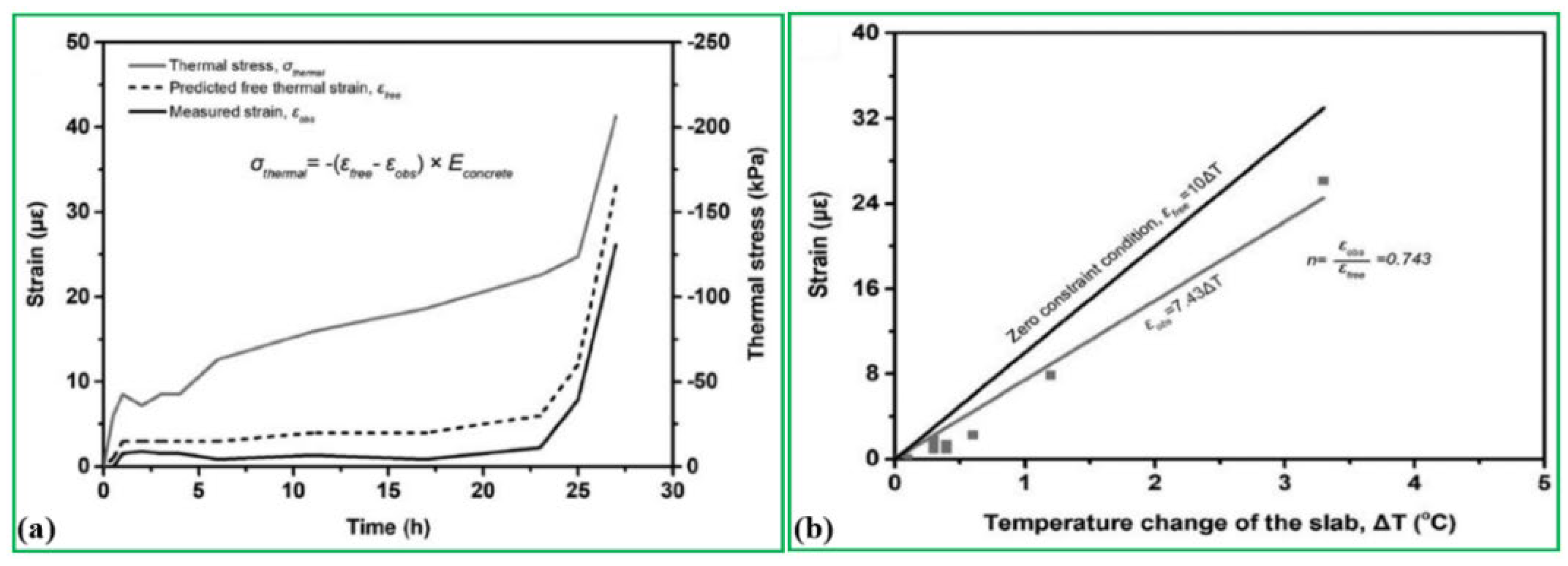
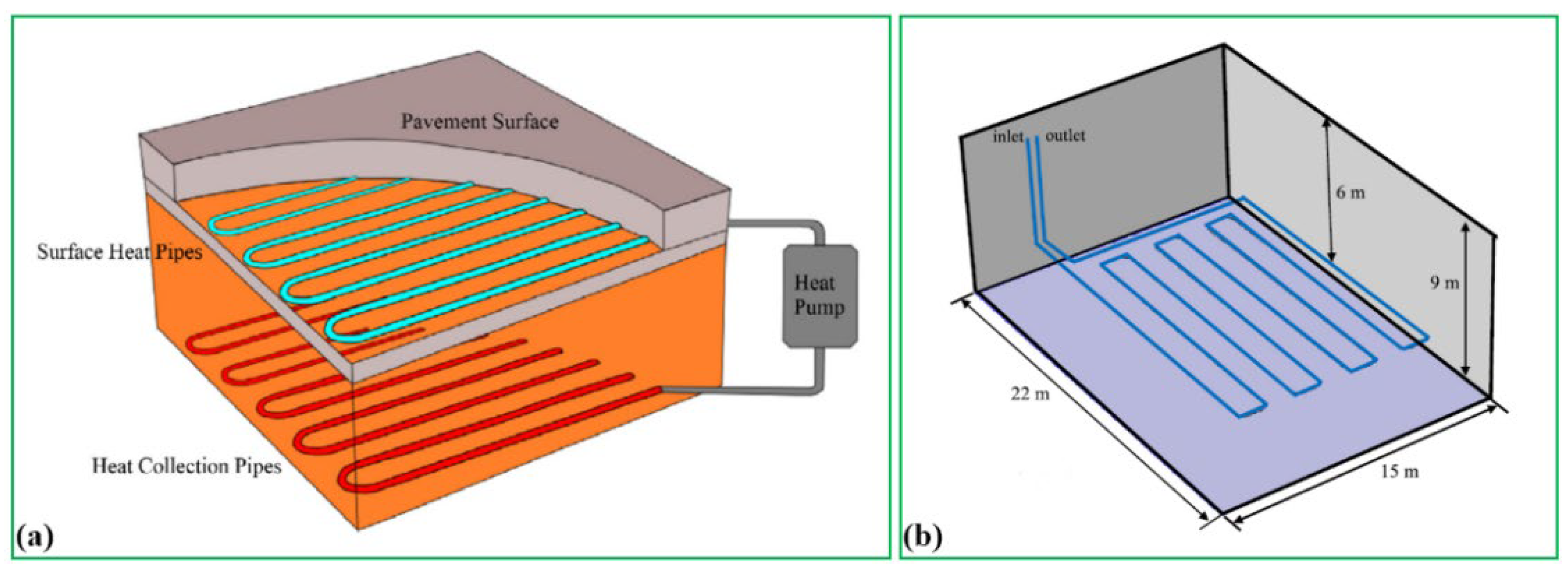
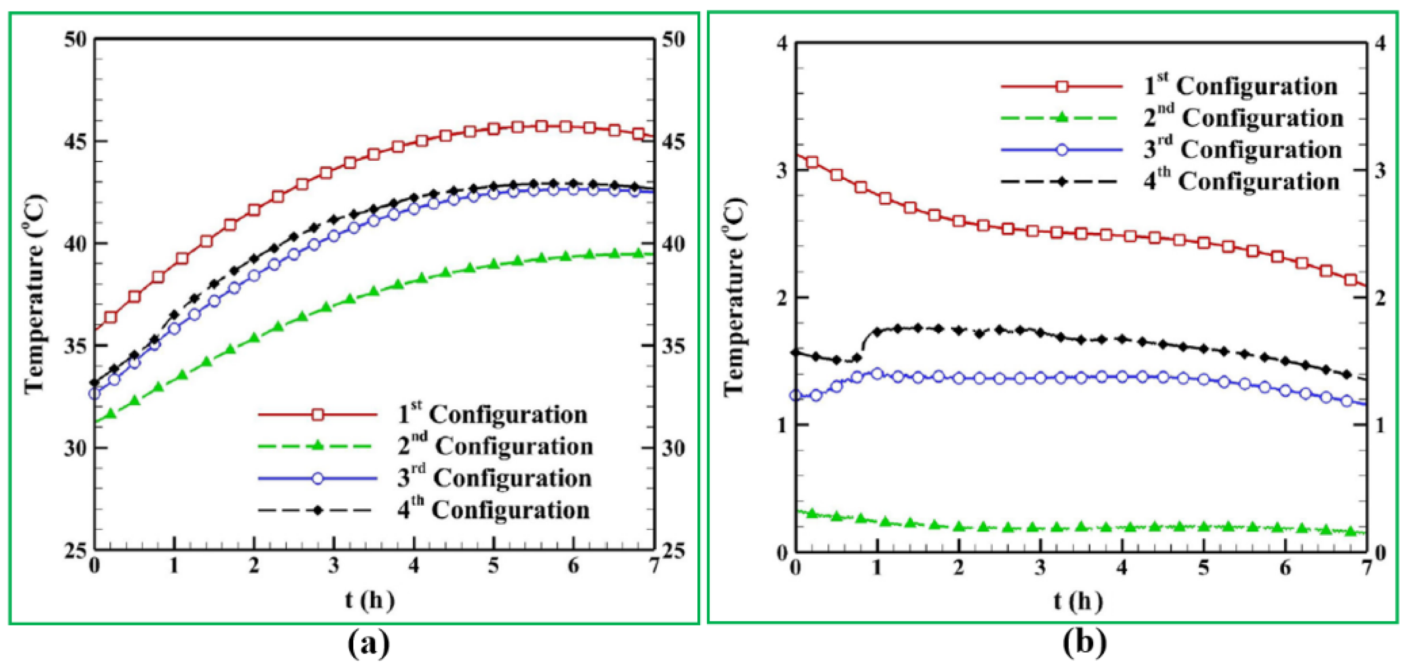
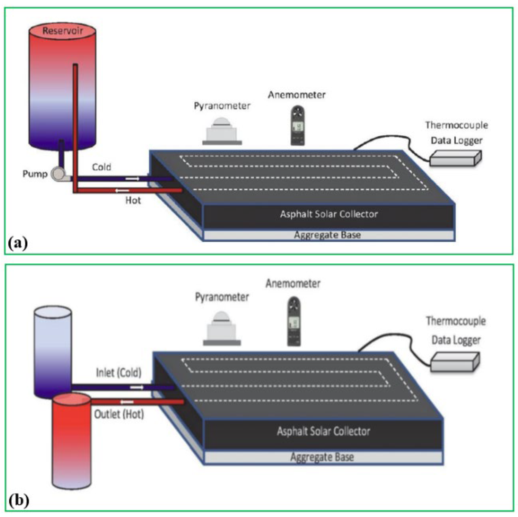
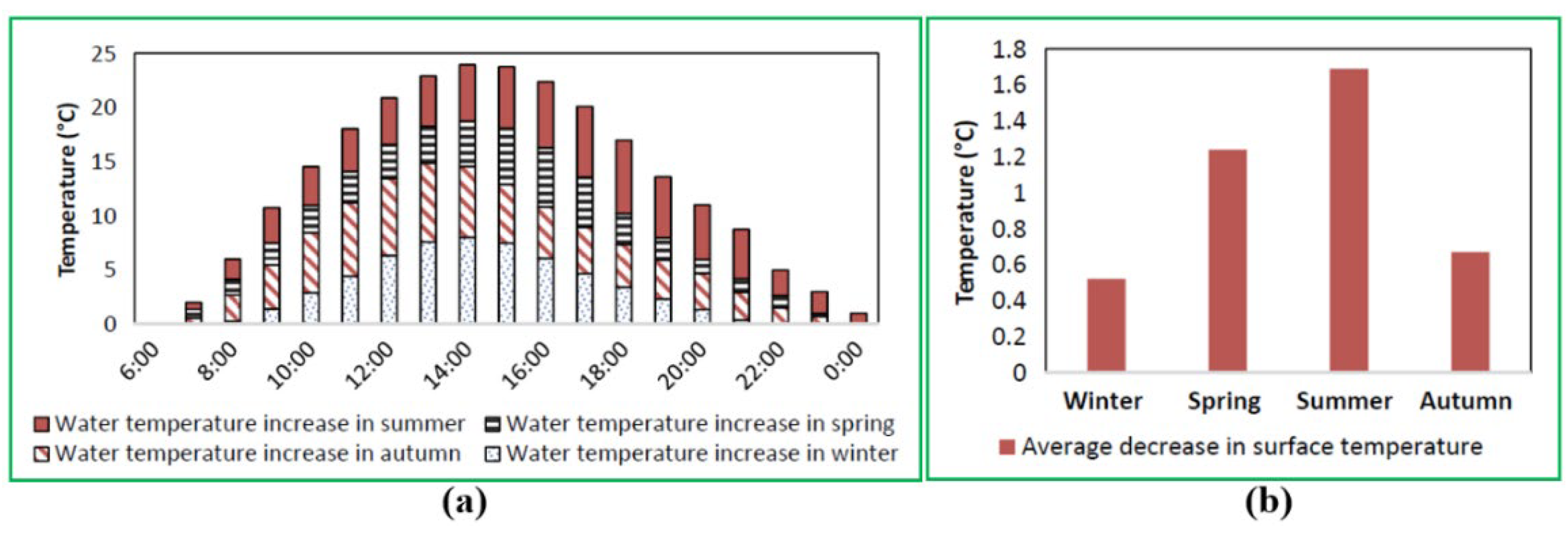
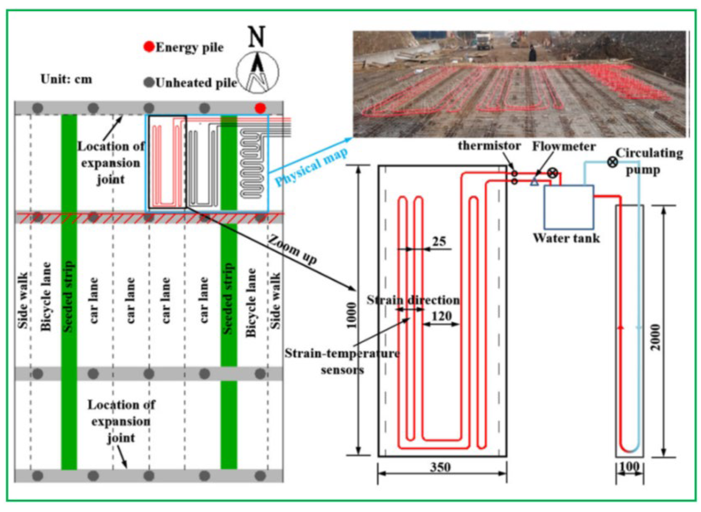
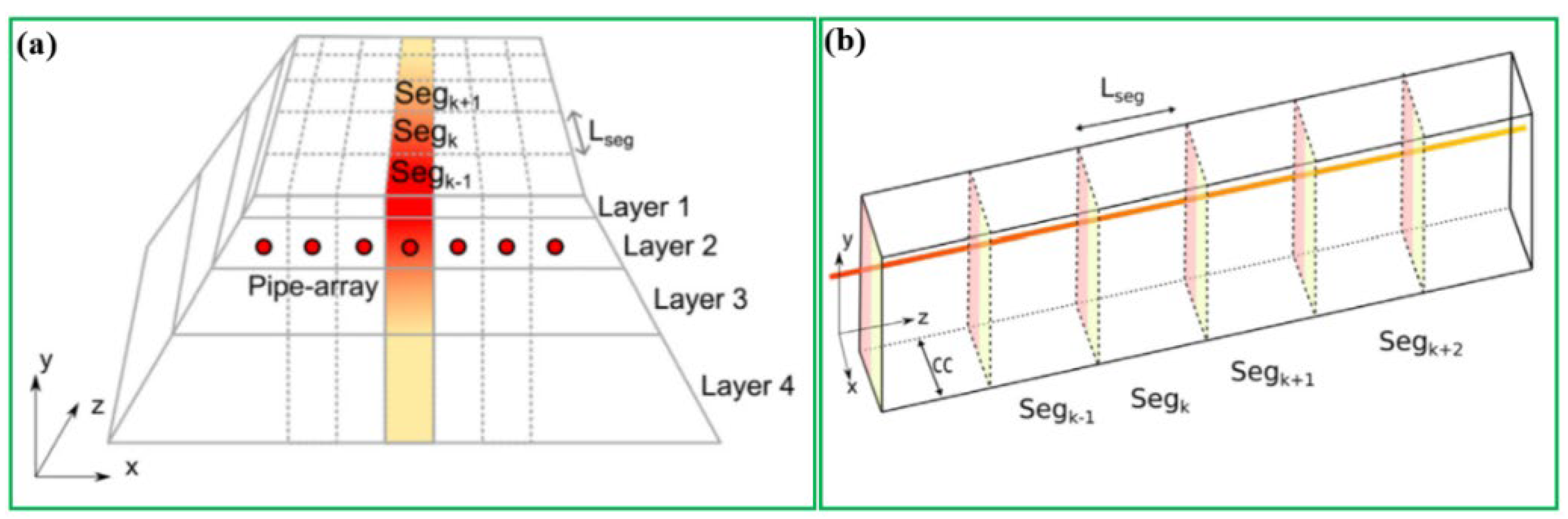
In another development, Kong et al. [31] experimentally tested a GRES for a bridge of 36 m by 26 m dimensions, that has two bicycle and four vehicle lanes. As presented in Figure 13, the GRES is mounted on the first span slab of the bridge and only half way is covered transversely. The pipe is a polyethylene (PE) tube that has the outer and inner diameters of 16 and 20 mm, which is embedded in the 100 mm thickness of concrete slab. Meanwhile, a thermal water tank is placed between the bridge and EP. The results illustrated in Figure 14a demonstrate that about 25.7% of the thermal expansion strain is limited via the unheated concrete slab, and the stress through the GRES reaches up to 206 kPa, which is far lower in comparison with the design parameter of the C40 concrete compressive strength of 19.1 MPa, as shown in Figure 14b.

3.1.2. Geothermal Pavement Energy System

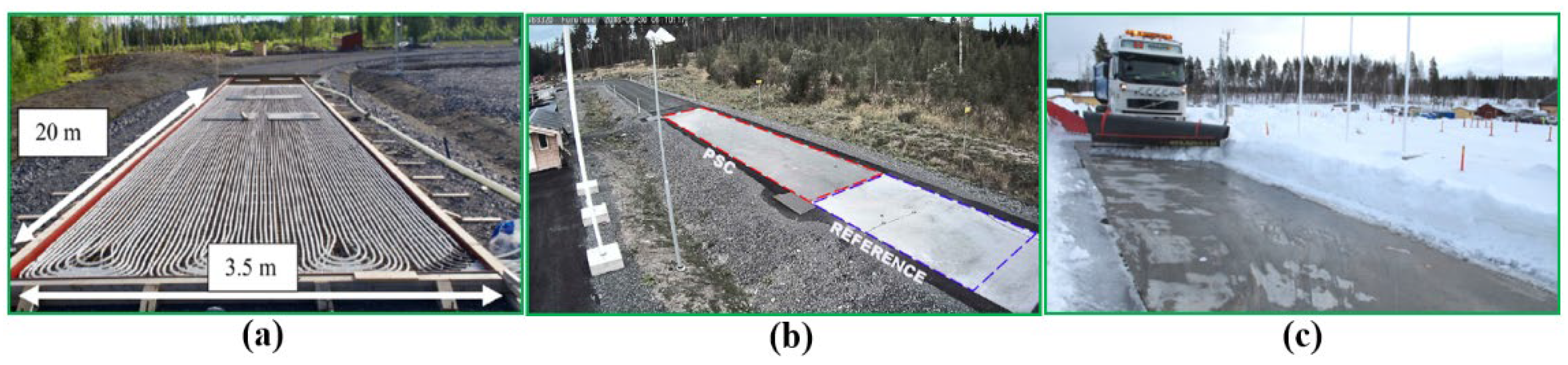
For the road pavement, Mirzanamadi et al. [32] implemented an experimental testing of the GRES to measure the pavement surface temperature based on Sweden’s weather condition. There is no noticeable infrastructure near the experimental site as displayed in Figure 15a, and therefore the shading impact of neighbouring infrastructure on the surface of the pavement is ignored; furthermore, the layers of the pavement and relevant parameters are given in Figure 15b.

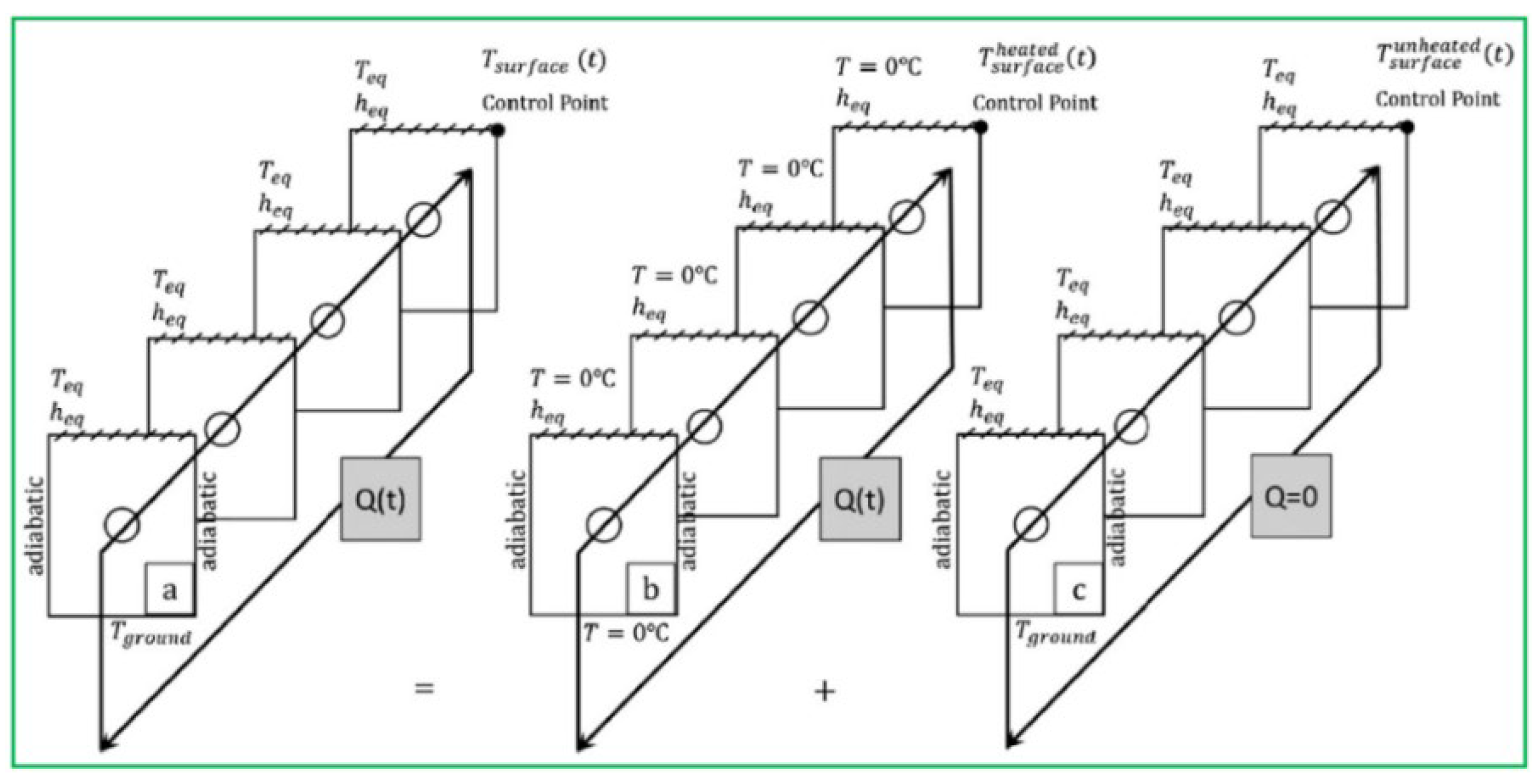
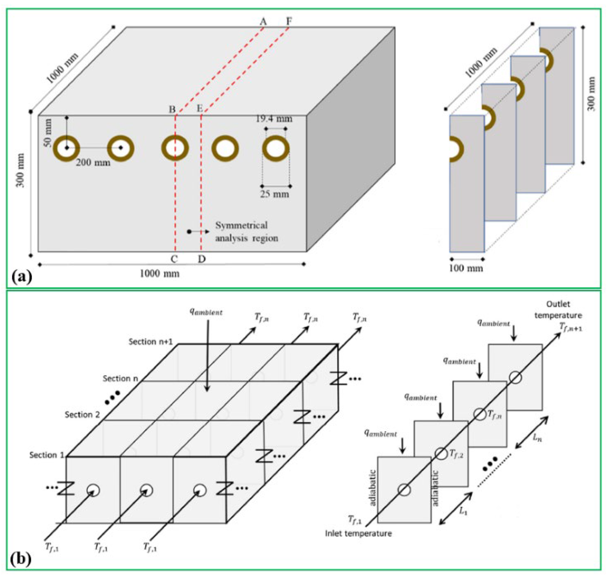
Afterwards, Mirzanamadi et al. [33] built a 3D heat transfer model of the GRES to investigate the unsteady anti-icing method on the basis of the superposition principle. Specifically, the model has a dimension of 1000 × 1000 × 300 mm (L × W × D) with 50 mm depth, a pipe distance of 200 mm is given in Figure 16a. For the purpose of reducing the computational time, the symmetrical section A-B-C-D-E-F is used to simulate the heat transfer process. According to Figure 16b, the 3D model is replaced by four 2D vertical cross sections that are serially linked to each other, the initial temperatures of the pavement bottom and top boundaries are set at 0 °C as given in Figure 17. The basic heat transfer equations are given in

Table 2. Hybrid 3D heat transfer model and the principle of superposition [33].

Description	Equations
Thermal resistance	${\mathrm{R}}_{\mathrm{e}\mathrm{q}-\mathrm{p}\mathrm{i}\mathrm{p}\mathrm{e}}={\mathrm{R}}_{\mathrm{p}\mathrm{i}\mathrm{p}\mathrm{e}}+{\mathrm{R}}_{\mathrm{i},\mathrm{j}}+{\mathrm{R}}_{\mathrm{P}\mathrm{W}\mathrm{S}}$ ${\mathrm{R}}_{\mathrm{p}\mathrm{i}\mathrm{p}\mathrm{e}}=\frac{\ln (\frac{{\mathrm{r}}_{\mathrm{o}\mathrm{u}\mathrm{t}\mathrm{e}\mathrm{r}}}{{\mathrm{r}}_{\mathrm{i}\mathrm{n}\mathrm{n}\mathrm{e}\mathrm{r}}})}{2\cdot \mathsf{\pi }\cdot {\mathsf{\lambda }}_{\mathrm{p}\mathrm{i}\mathrm{p}\mathrm{e}}}$ ${\mathrm{R}}_{\mathrm{i},\mathrm{j}}=\frac{\ln (\frac{{\mathrm{r}}_{\mathrm{i},\mathrm{j}}}{{\mathrm{r}}_{\mathrm{o}\mathrm{u}\mathrm{t}\mathrm{e}\mathrm{r}}})}{2\cdot \mathsf{\pi }\cdot {\mathsf{\lambda }}_{\mathrm{i},\mathrm{j}}}$ ${\mathrm{R}}_{\mathrm{P}\mathrm{W}\mathrm{S}}=\frac{1}{\mathsf{\pi }\cdot {\mathsf{\lambda }}_{\mathrm{f}}\cdot \mathrm{N}\mathrm{u}}$
Temperature distribution of working fluid within the pipe	${\mathrm{T}}_{\mathrm{e}\mathrm{q}-\mathrm{p}\mathrm{i}\mathrm{p}\mathrm{e}}={\mathrm{T}}_{\mathrm{f}}-{\mathrm{q}}_{\mathrm{i},\mathrm{j}}\cdot {\mathrm{R}}_{\mathrm{e}\mathrm{q}-\mathrm{p}\mathrm{i}\mathrm{p}\mathrm{e}}$
Outlet fluid temperature	${\mathrm{T}}_{\mathrm{f},\mathrm{n}+1}^{\mathrm{t}}={\mathrm{T}}_{\mathrm{e}\mathrm{q}-\mathrm{p}\mathrm{i}\mathrm{p}\mathrm{e},\mathrm{n}}^{\mathrm{t}}+({\mathrm{T}}_{\mathrm{f},\mathrm{n}}^{\mathrm{t}}\mathrm{p}{\mathrm{T}}_{\mathrm{e}\mathrm{q}-\mathrm{p}\mathrm{i}\mathrm{p}\mathrm{e},\mathrm{n}}^{\mathrm{t}})\cdot {\mathrm{e}}^{-({\mathrm{L}}_{\mathrm{n}}/{\mathrm{l}}_{\mathrm{n}})}$ ${\mathrm{l}}_{\mathrm{n}}={\mathrm{R}}_{\mathrm{e}\mathrm{q}-\mathrm{p}\mathrm{i}\mathrm{p}\mathrm{e}}\cdot {\mathsf{\nu }}_{\mathrm{f}}\cdot \mathsf{\pi }\cdot {\mathrm{r}}_{\mathrm{i}\mathrm{n}\mathrm{n}\mathrm{e}\mathrm{r}}^2\cdot {\mathsf{\rho }}_{\mathrm{f}}\cdot {\mathrm{c}}_{\mathrm{p},\mathrm{f}}$
Principle of superposition	${\mathrm{T}}_{\mathrm{s}\mathrm{u}\mathrm{r}\mathrm{f}\mathrm{a}\mathrm{c}\mathrm{e}}(\mathrm{t})={\mathrm{T}}_{\mathrm{s}\mathrm{u}\mathrm{r}\mathrm{f}\mathrm{a}\mathrm{c}\mathrm{e}}^{\mathrm{h}\mathrm{e}\mathrm{a}\mathrm{t}\mathrm{e}\mathrm{d}}(\mathrm{t})+{\mathrm{T}}_{\mathrm{s}\mathrm{u}\mathrm{r}\mathrm{f}\mathrm{a}\mathrm{c}\mathrm{e}}^{\mathrm{u}\mathrm{n}\mathrm{h}\mathrm{e}\mathrm{a}\mathrm{t}\mathrm{e}\mathrm{d}}(\mathrm{t})$

.

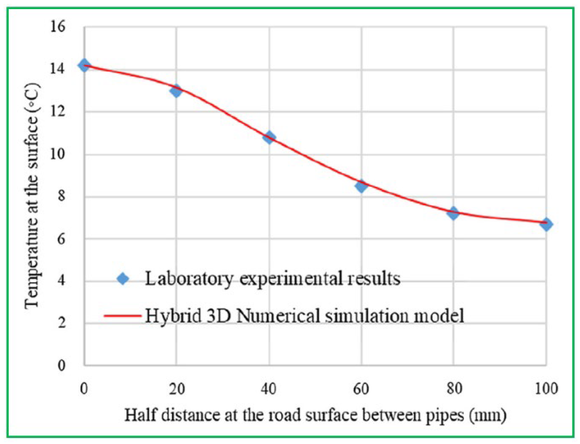
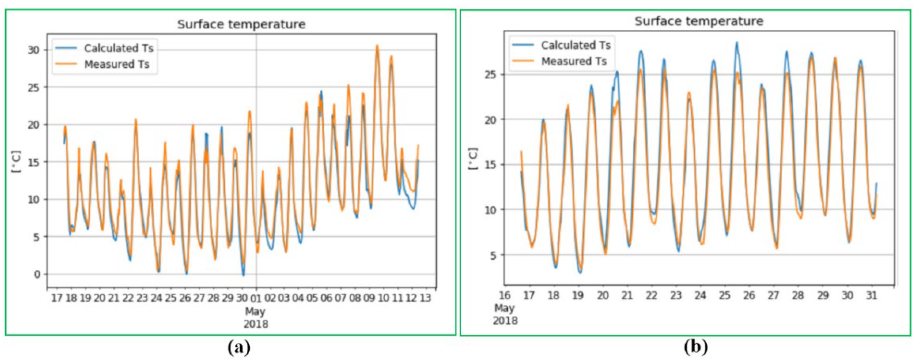
It is found from Figure 18 that the numerical results are in agreement with the testing data, with a maximum difference of 2.4%. Based on the hybrid 3D model, Mirzanamadi et al. [34] investigated the system performance for de-icing pavement surface for a 15-year operation period, and found that the maximum value associated with the solar energy harvested is 30 kWh/m² in July whereas the minimum value is 0.5 kWh/m² in April. Furthermore, the maximum energy demand is 25 kWh/m² in December and January, while the mean value of the required energy and the residual number of hours of slippery conditions from October and March are 1.3 kWh/m² and 9 h, respectively.

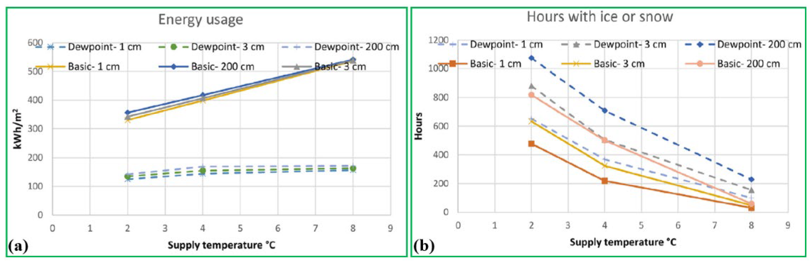
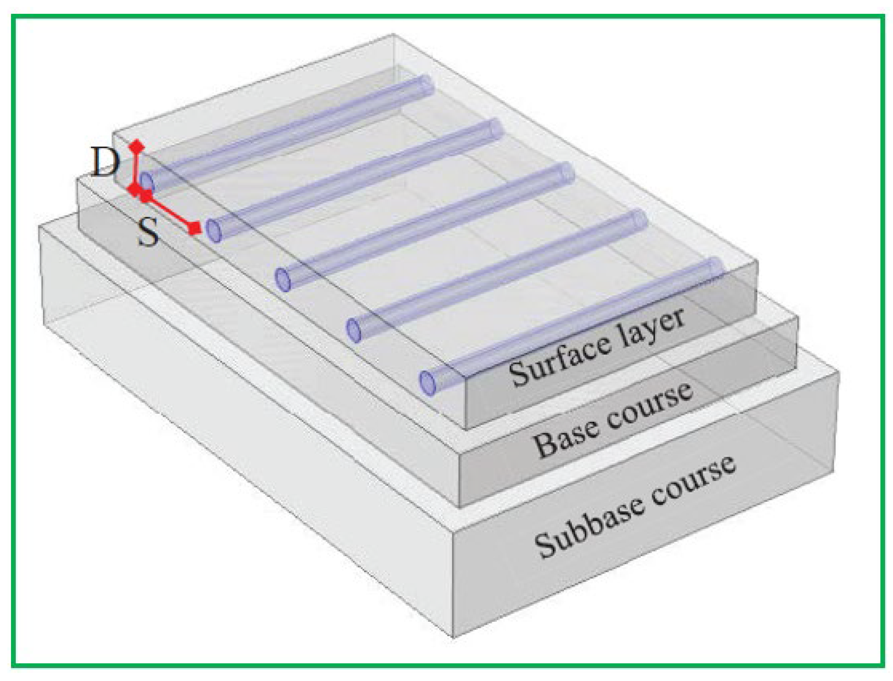
Adl-Zarrabi et al. [35] developed a 3D COMSOL model of a GRES to study the effect of the pipe position on de-icing performance as presented in Figure 19. The system involves a surface layer of 150 mm thickness, the base of 250 mm thickness and subbase courses as well as pipes of 1.5mm thickness, which are buried in the concrete slab. The results in Figure 20a show that the required time for melting the snow on the pavement could be enhanced speedily when the distance between pipes exceeds 200 mm. In other words, the best distance between pipes should be less than 200 mm. Additionally, as depicted in Figure 20b, there is little effect of the pipe depth on the anti-icing process when its depth is lower than 100 mm.

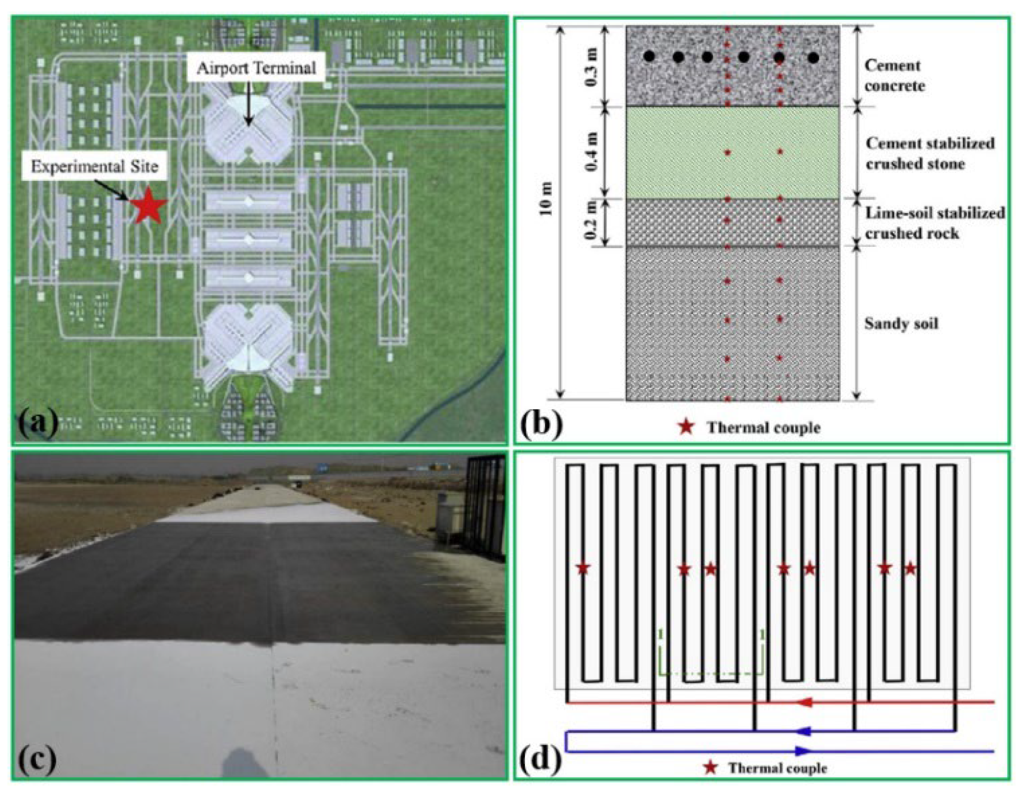
Xu et al. [36] setup a numerical model of the GRES to analyse the influences of preheating time and snowfall rate on the snow melting performance at Beijing New Capital International Airport as shown in Figure 21. The whole area of the experimental site is 90 m², with a stainless steel pipe of 32 mm diameter, 0.4 m length and a depth of 0.08 m embedded underground. A geothermal heat pump unit with a rated power of 50 kW is utilized to warm 25% of ethylene glycol solution. The basic equations of water transport, heat transport and error analysis are presented in

Table 3. GRES model [36].

Description	Equations
Water transport	$\frac{\partial \mathsf{\theta }}{\partial \mathsf{\tau }}=\nabla ({\mathrm{D}}_{\mathrm{l}}(\mathsf{\theta })\nabla \mathsf{\theta })+\nabla ({\mathrm{D}}_{\mathrm{l}}(\mathrm{T})\nabla \mathrm{T})-\frac{\partial \mathrm{K}(\mathsf{\theta })}{\partial \mathrm{y}}+\nabla ({\mathrm{D}}_{\mathrm{v}}(\mathsf{\theta })\nabla \mathsf{\theta })+\nabla ({\mathrm{D}}_{\mathrm{v}}(\mathrm{T})\nabla \mathrm{T})$ $\mathrm{K}{(\frac{\mathsf{\theta }-{\mathsf{\theta }}_{\mathrm{r}}}{{\mathsf{\theta }}_{\mathrm{s}}-{\mathsf{\theta }}_{\mathrm{r}}})}^{\mathrm{n}+2+\frac{2}{\mathrm{a}}}=\mathrm{K}(\mathsf{\theta })$ ${\mathrm{D}}_{\mathrm{v}}(\mathsf{\theta })=\frac{1}{{\mathsf{\rho }}_{\mathrm{w}}}{\mathrm{D}}_0\mathsf{\alpha }\mathrm{b}{\mathsf{\rho }}_0\frac{\partial {\mathrm{h}}_0}{\partial \mathsf{\theta }}$ ${\mathrm{D}}_{\mathrm{l}}(\mathsf{\theta })=\mathrm{K}(\mathsf{\theta })\frac{\partial \mathsf{\psi }}{\partial \mathsf{\theta }}$
Heat transport	$\frac{\partial }{\partial \mathsf{\tau }}(\mathrm{C}(\mathsf{\theta })\mathrm{T})=\frac{\partial }{\partial \mathrm{x}}(\mathsf{\lambda }(\mathsf{\theta })\frac{\partial \mathrm{t}}{\mathrm{x}})+\frac{\partial }{\partial \mathrm{y}}(\mathsf{\lambda }(\mathsf{\theta })\frac{\partial \mathrm{t}}{\mathrm{y}})$ $\mathrm{C}(\mathsf{\theta })={\mathrm{C}}_{\mathrm{d}\mathrm{r}\mathrm{y}}+\frac{\mathsf{\theta }}{{\mathsf{\theta }}_{\mathrm{s}}}({\mathrm{C}}_{\mathrm{s}\mathrm{a}\mathrm{t}}-{\mathrm{C}}_{\mathrm{d}\mathrm{r}\mathrm{y}})$ $\mathsf{\lambda }(\mathsf{\theta })={\mathsf{\lambda }}_{\mathrm{d}\mathrm{r}\mathrm{y}}+{\mathrm{K}}_{\mathrm{e}}({\mathsf{\lambda }}_{\mathrm{s}\mathrm{a}\mathrm{t}}-{\mathsf{\lambda }}_{\mathrm{d}\mathrm{r}\mathrm{y}})$
RMSE	$\mathrm{R}\mathrm{M}\mathrm{S}\mathrm{E}=\sqrt{\frac{1}{\mathrm{n}}{\displaystyle \sum {({\mathrm{N}}_{\mathrm{i}}-{\mathrm{O}}_{\mathrm{i}})}^2}}$
ME	$\mathrm{M}\mathrm{E}=\frac{1}{\mathrm{n}}{\displaystyle \sum ({\mathrm{N}}_{\mathrm{i}}-{\mathrm{O}}_{\mathrm{i}})}$

. The results indicate that the percentage of snow-free hours during snowfall at four preheating times is improved ranging from 1.3% to 5.6%. As a result, it is necessary to adjust the snow melting target by the traffic capacity as the design alternatives.

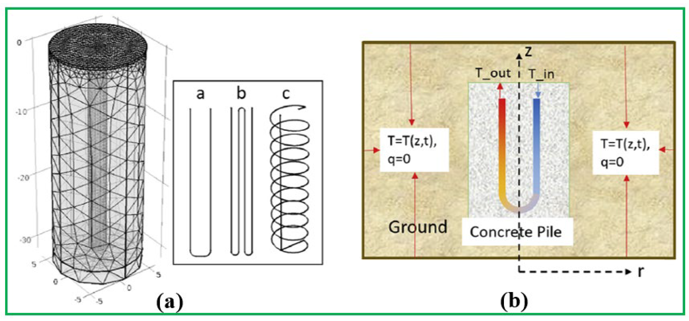
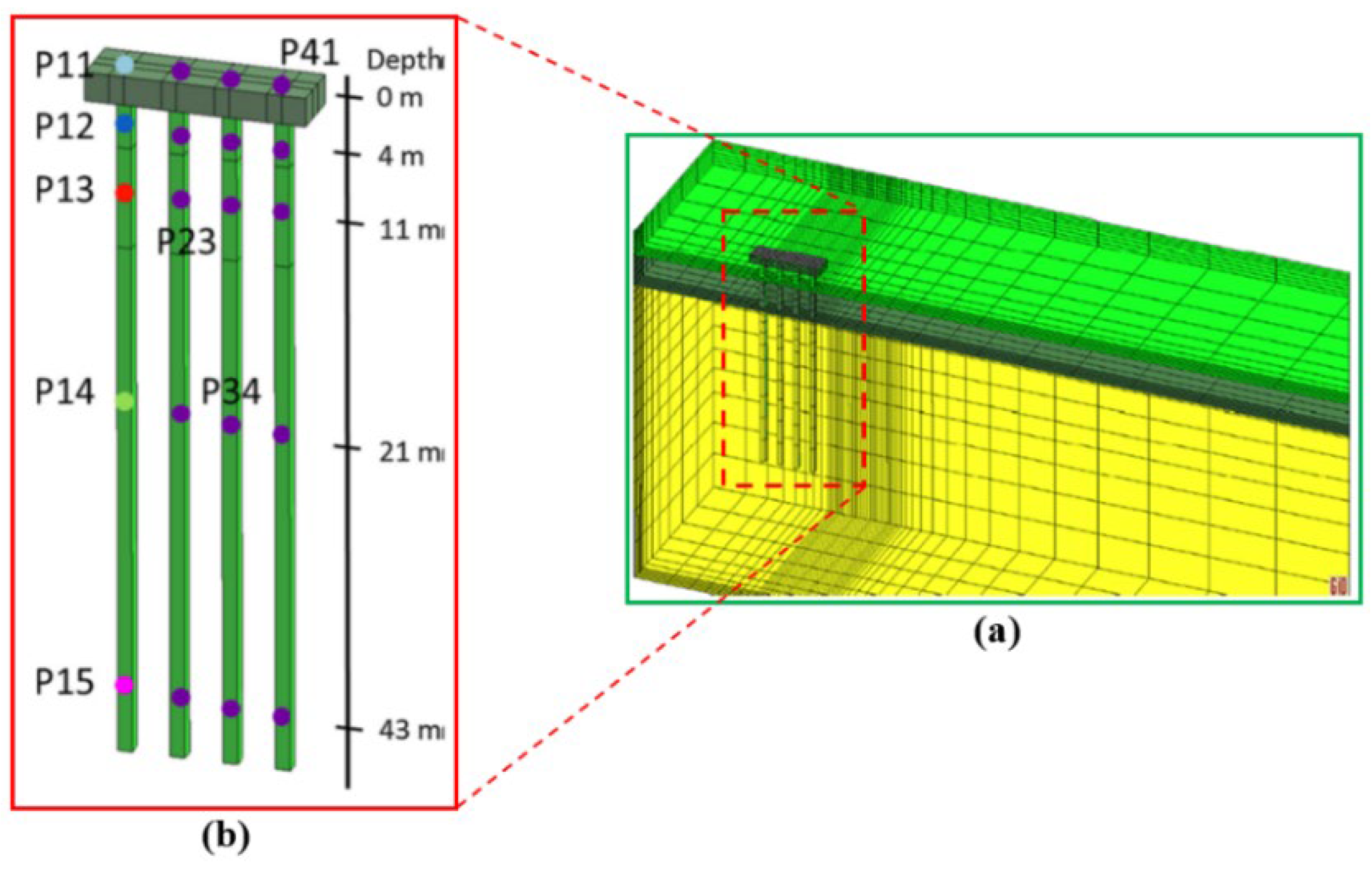
Han and Yu [37] set up a 3D model of the GRES with EP technology to assess the energy extraction rate and required pile number for three configurations in the USA. As shown in Figure 22a, the soil domain is defined as a cylinder and has a diameter of 12 m. The Dirichlet boundary condition is used as the borders of the calculation field with the magnitude set to be the undisturbed soil temperature as presented in Figure 22b.

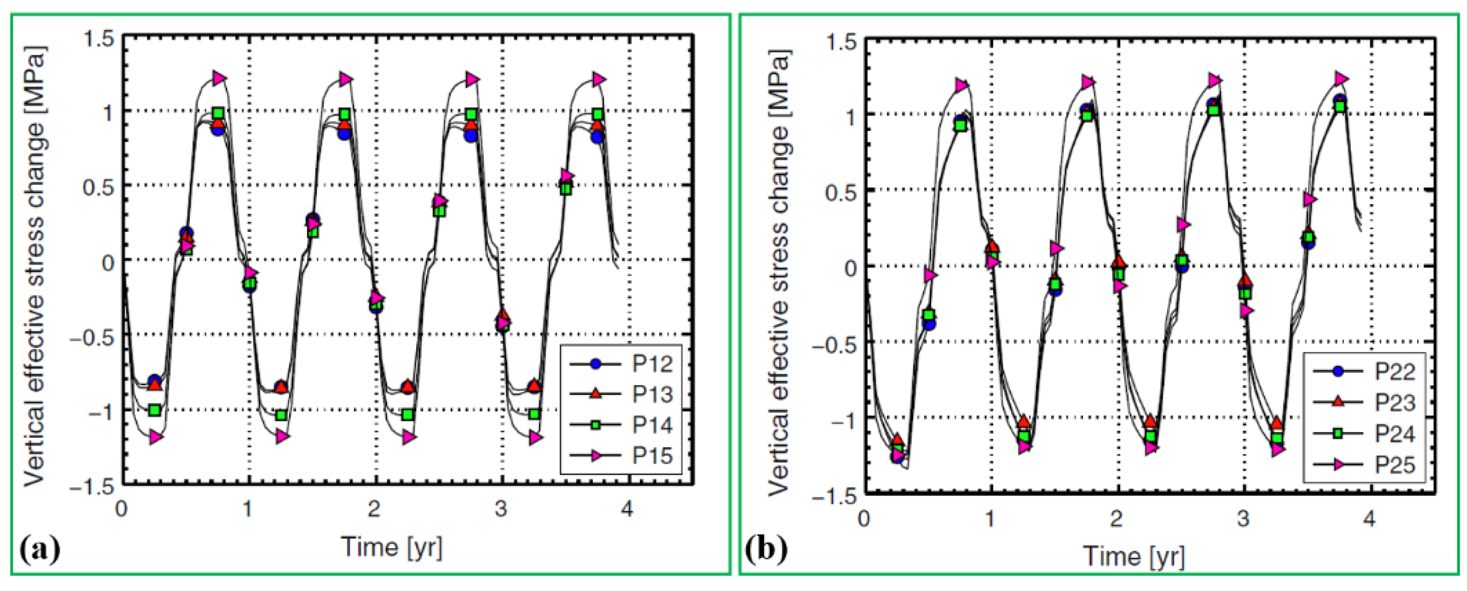
Additionally, it can be found from Figure 23 that high soil temperature contributes to extracting energy and producing high-temperature outlet fluid; moreover, the spiral pipe shape (type c) could extract more heat in comparison with U-shape (type a) and W-shape (type b) pipes; this means that the spiral pipe shape is the best choice for the system to improve snow melting performance under the constraint of limited pile length.

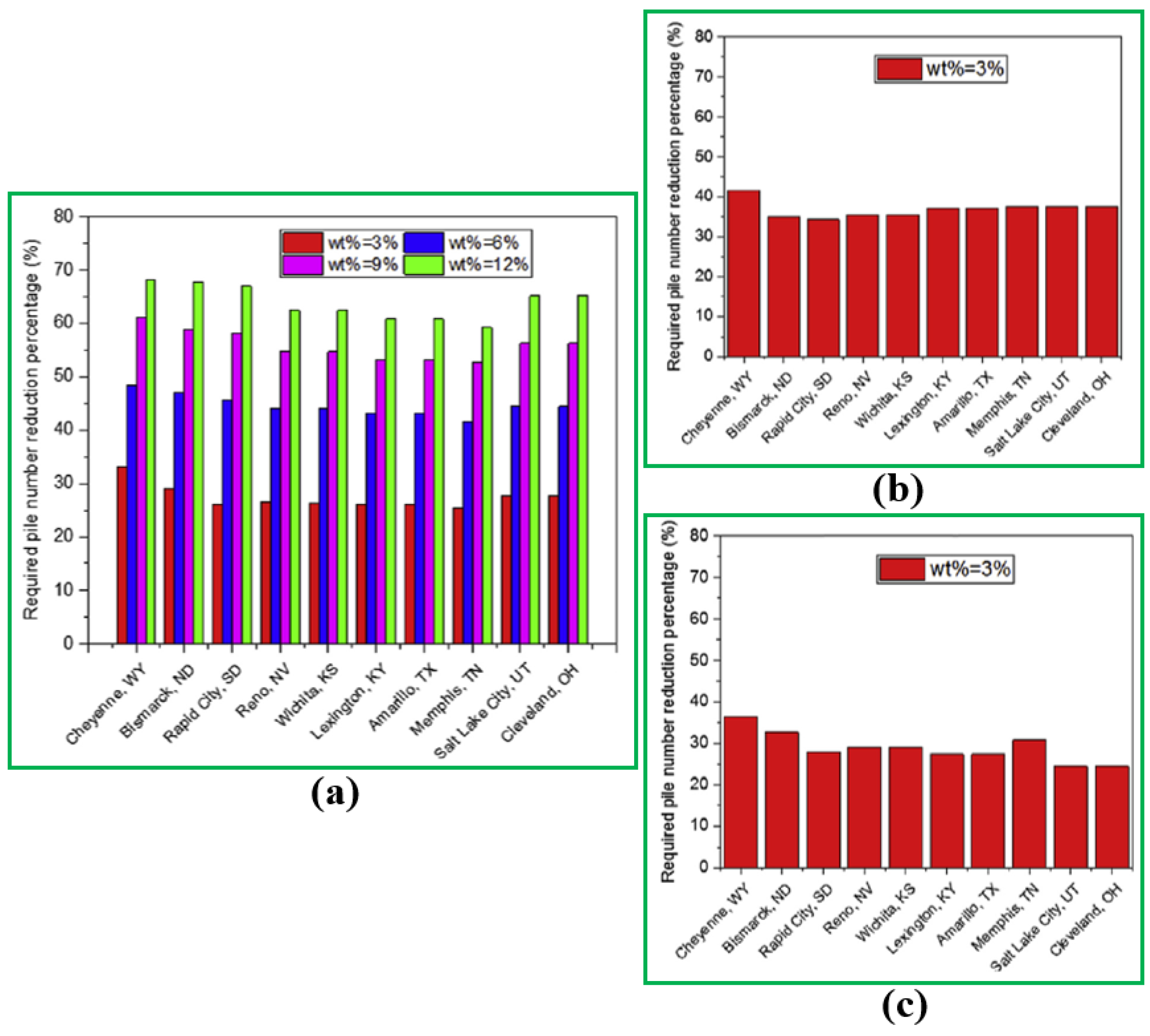
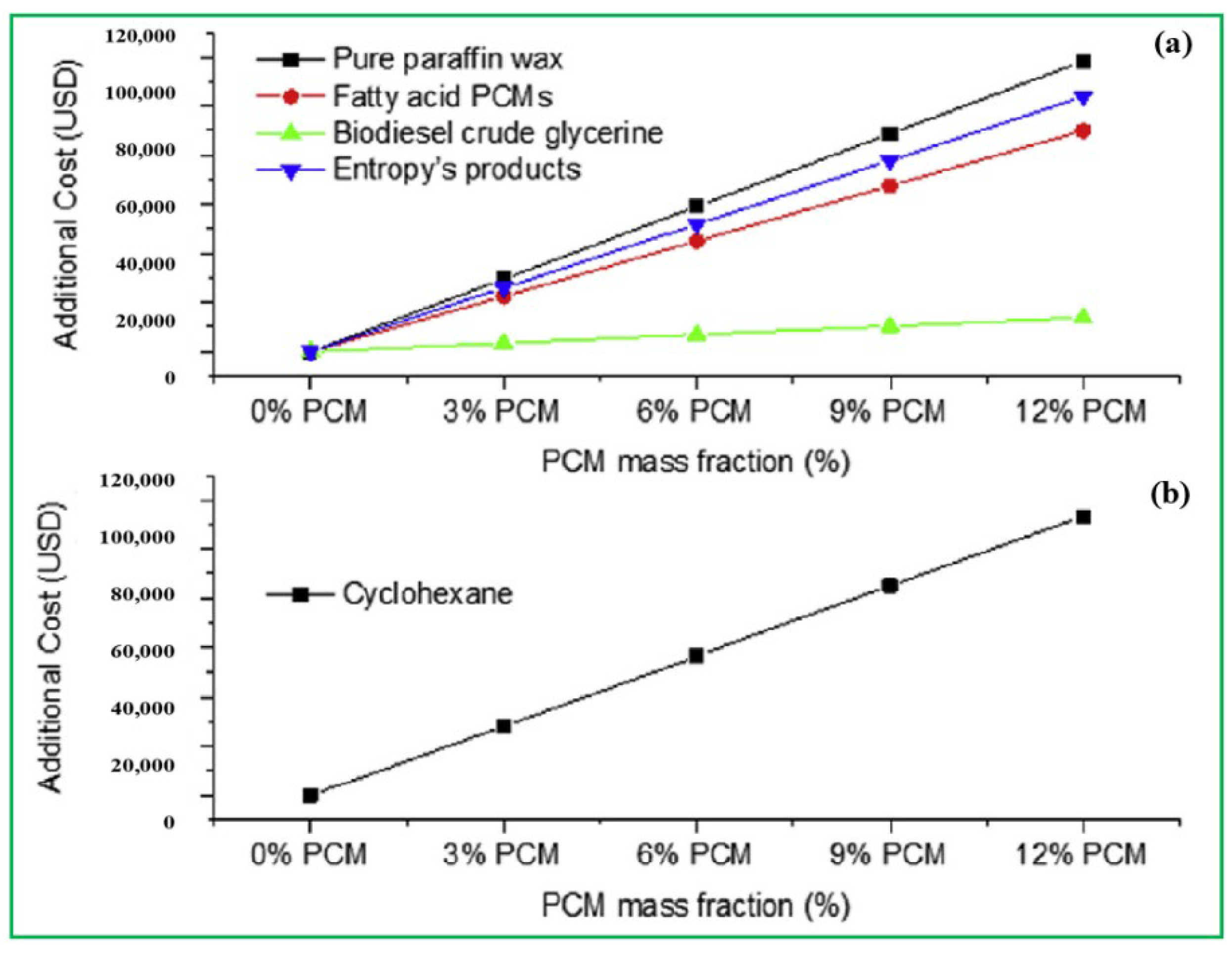
In addition, Han and Yu [38] modified the GRES with EP by integrating a phase change material (PCM) in order to enhance system performance as shown in Figure 24. The equations of the modified GRES model are given in

Table 4. PCM modified model [38].

Description	Equations
PCM model	$\mathsf{\rho }=\mathsf{\theta }(\mathrm{T}){\mathsf{\rho }}_{\mathrm{p}\mathrm{h}\mathrm{a}\mathrm{s}\mathrm{e}1}+[1-\mathsf{\theta }(\mathrm{T})]{\mathsf{\rho }}_{\mathrm{p}\mathrm{h}\mathrm{a}\mathrm{s}\mathrm{e}2}$ $\mathrm{k}=\mathsf{\theta }(\mathrm{T}){\mathrm{k}}_{\mathrm{p}\mathrm{h}\mathrm{a}\mathrm{s}\mathrm{e}1}+[1-\mathsf{\theta }(\mathrm{T})]{\mathrm{k}}_{\mathrm{p}\mathrm{h}\mathrm{a}\mathrm{s}\mathrm{e}2}$ ${\mathrm{C}}_{\mathrm{p}}=\frac{1}{\mathsf{\rho }}\{\mathsf{\theta }(\mathrm{T}){\mathsf{\rho }}_{\mathrm{p}\mathrm{h}\mathrm{a}\mathrm{s}\mathrm{e}1}{\mathrm{C}}_{\mathrm{p},\mathrm{p}\mathrm{h}\mathrm{a}\mathrm{s}\mathrm{e}1}+[1-\mathsf{\theta }(\mathrm{T}){\mathsf{\rho }}_{\mathrm{p}\mathrm{h}\mathrm{a}\mathrm{s}\mathrm{e}2}{\mathrm{C}}_{\mathrm{p},\mathrm{p}\mathrm{h}\mathrm{a}\mathrm{s}\mathrm{e}2}]\}+\mathrm{L}\frac{\partial {\mathsf{\alpha }}_{\mathrm{m}}(\mathrm{T})}{\partial \mathrm{T}}$ ${\mathsf{\alpha }}_{\mathrm{m}}(\mathrm{T})=\frac{1}{2}\frac{[1-\mathsf{\theta }(\mathrm{T})]{\mathsf{\rho }}_{\mathrm{p}\mathrm{h}\mathrm{a}\mathrm{s}\mathrm{e}2}-[\mathsf{\theta }(\mathrm{T}){\mathsf{\rho }}_{\mathrm{p}\mathrm{h}\mathrm{a}\mathrm{s}\mathrm{e}1}]}{\mathsf{\theta }(\mathrm{T}){\mathsf{\rho }}_{\mathrm{p}\mathrm{h}\mathrm{a}\mathrm{s}\mathrm{e}1}{\mathrm{C}}_{\mathrm{p},\mathrm{p}\mathrm{h}\mathrm{a}\mathrm{s}\mathrm{e}1}+[1-\mathsf{\theta }(\mathrm{T}){\mathsf{\rho }}_{\mathrm{p}\mathrm{h}\mathrm{a}\mathrm{s}\mathrm{e}2}]}$ ${\mathrm{M}}_{\mathrm{p}\mathrm{h}\mathrm{a}\mathrm{s}\mathrm{e}1}=(1-\mathrm{w}\mathrm{t}\%){\mathrm{M}}_{\mathrm{c}\mathrm{o}\mathrm{n}\mathrm{c}\mathrm{r}\mathrm{e}\mathrm{t}\mathrm{e}}+\mathrm{w}\mathrm{t}\%{\mathrm{M}}_{\mathrm{P}\mathrm{C}\mathrm{M},\mathrm{p}\mathrm{h}\mathrm{a}\mathrm{s}\mathrm{e}1}$ ${\mathrm{M}}_{\mathrm{p}\mathrm{h}\mathrm{a}\mathrm{s}\mathrm{e}1}=(1-\mathrm{w}\mathrm{t}\%){\mathrm{M}}_{\mathrm{c}\mathrm{o}\mathrm{n}\mathrm{c}\mathrm{r}\mathrm{e}\mathrm{t}\mathrm{e}}+\mathrm{w}\mathrm{t}\%{\mathrm{M}}_{\mathrm{P}\mathrm{C}\mathrm{M},\mathrm{p}\mathrm{h}\mathrm{a}\mathrm{s}\mathrm{e}1}$
Heat transport within EP	$\mathsf{\rho }{\mathrm{C}}_{\mathrm{p}}\frac{\partial \mathrm{T}}{\partial \mathrm{t}}+\nabla \cdot (-\mathrm{k}\nabla \mathrm{T})=-{\mathrm{Q}}_{\mathrm{w}\mathrm{a}\mathrm{l}\mathrm{l}}$

. As shown in Figure 25, the required numbers of PCM piles for U-, W- and spiral-shape pipes significantly reduce in comparison with those without PCM attached (wt % = 0). The utilization of 3% PCM additive by mass fraction leads to a 25–35% drop in the needed number of piles for the designated cities based on design conditions, and the usage of 12% PCM decreases the pile number by 60–70%; this means that the soil temperature and pipe configuration layout have an influence on the needed number of piles of the modified GRES.

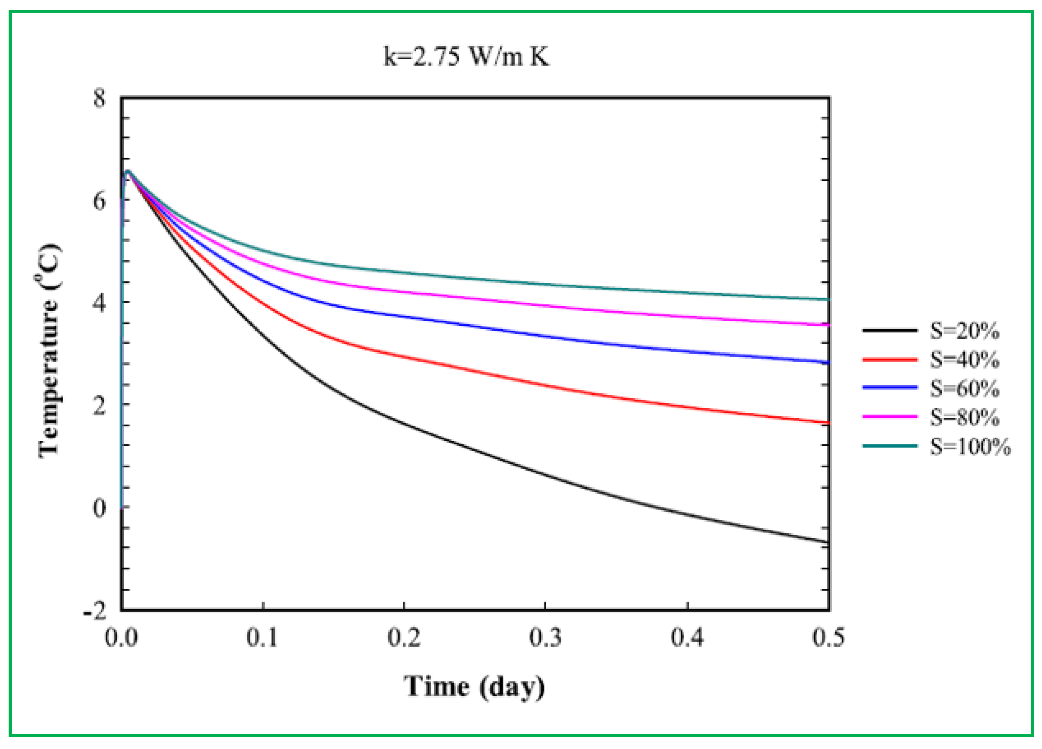
In another study [39], a finite element GRES model setup to investigate the outlet fluid temperature variation based on USA’s climate condition. As given in Figure 26, the system includes a heat pump and horizontal pipe loops that are laid under the soil at a depth of 6 m. Results confirm that the outlet fluid temperature could be kept higher than 4 °C when the soil is at full saturation, as indicated in Figure 27. On the other hand, the outlet fluid temperature could fall to −0.7 °C when the soil is completely dry; this implies that a dry soil is not an ideal medium to embed pipes within the soil layer.

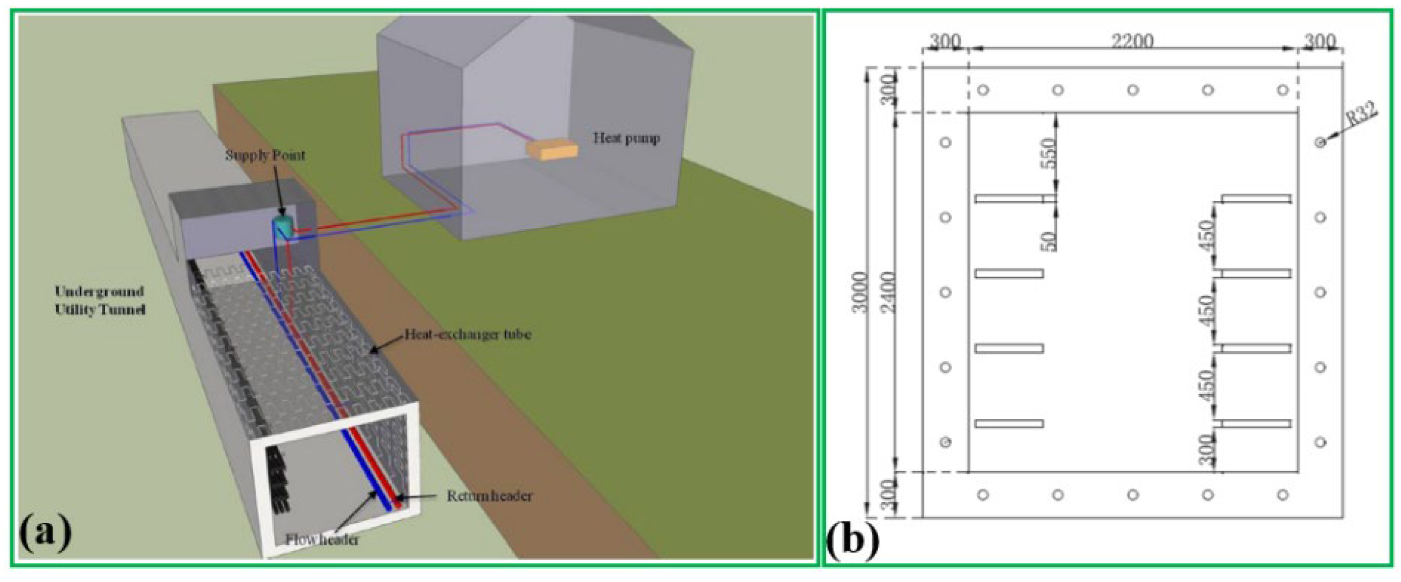
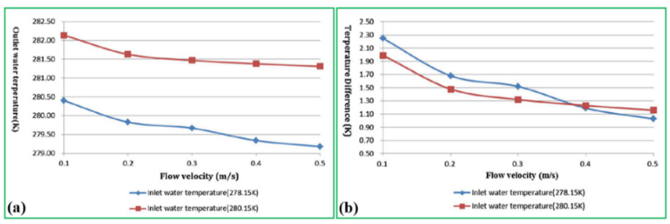
Yang et al. [40] developed a GRSE model for the underground utility tunnel (UUT) to extract heat from the soil and absorb waste heat within the tunnel. As exhibited in Figure 28, the UUT is constructed at a depth of 3–6 m under the urban roadway, which is deeper compared with the frozen soil layer. The dimension of the UUT is 3.0 × 2.8 m with 0.3 m of wall thickness. As indicated in Figure 29, the model results reflect that the outlet fluid temperature dramatically reduces while the maximum temperature difference between inlet and outlet is approximately 1 K when the inlet fluid temperature and flow velocity vary in the ranges of 280.15 K to 278.15 K and 0.1 m/L to 0.5 m/L, respectively; this suggests that the lower inlet water temperature and wind velocity improve the efficiency of heat transfer.

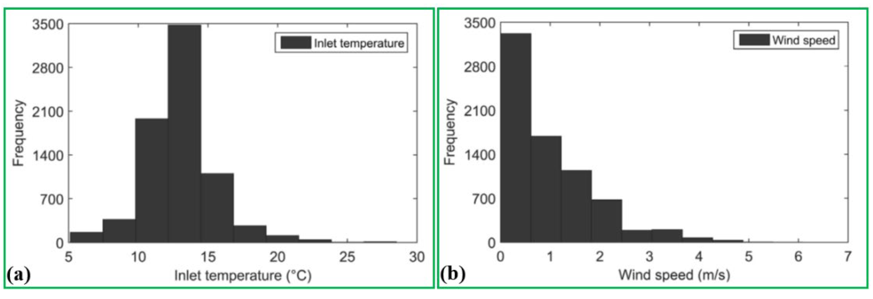
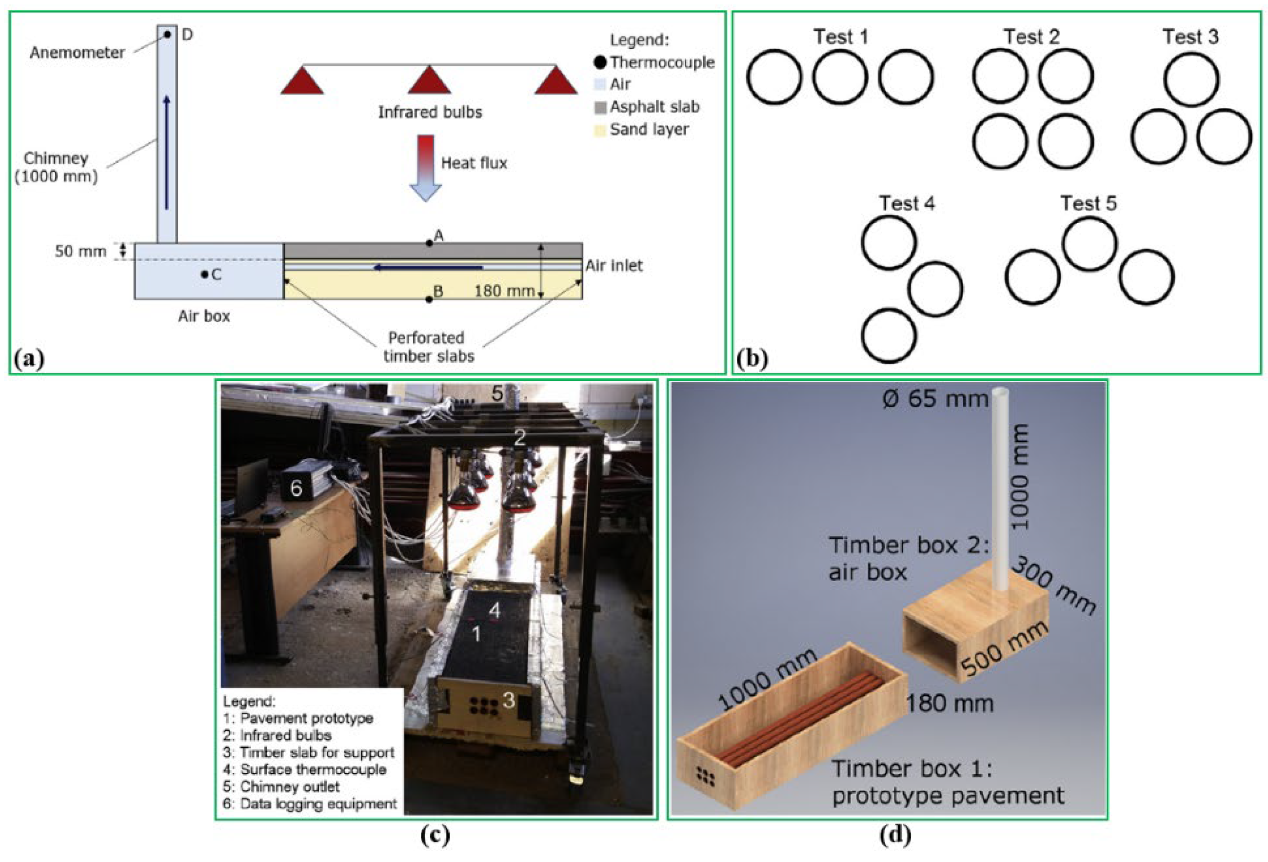
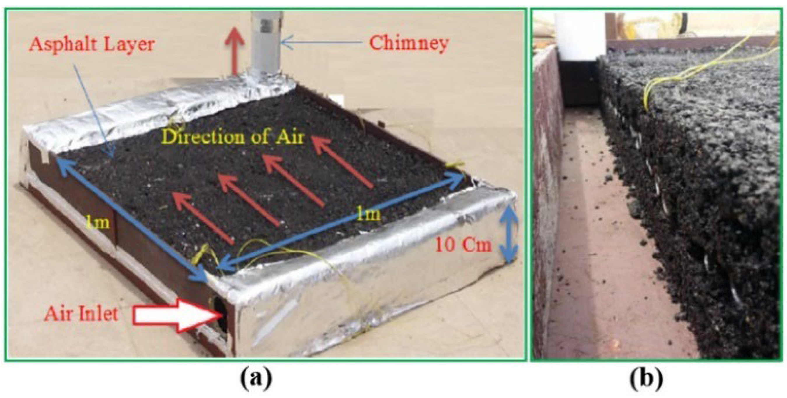
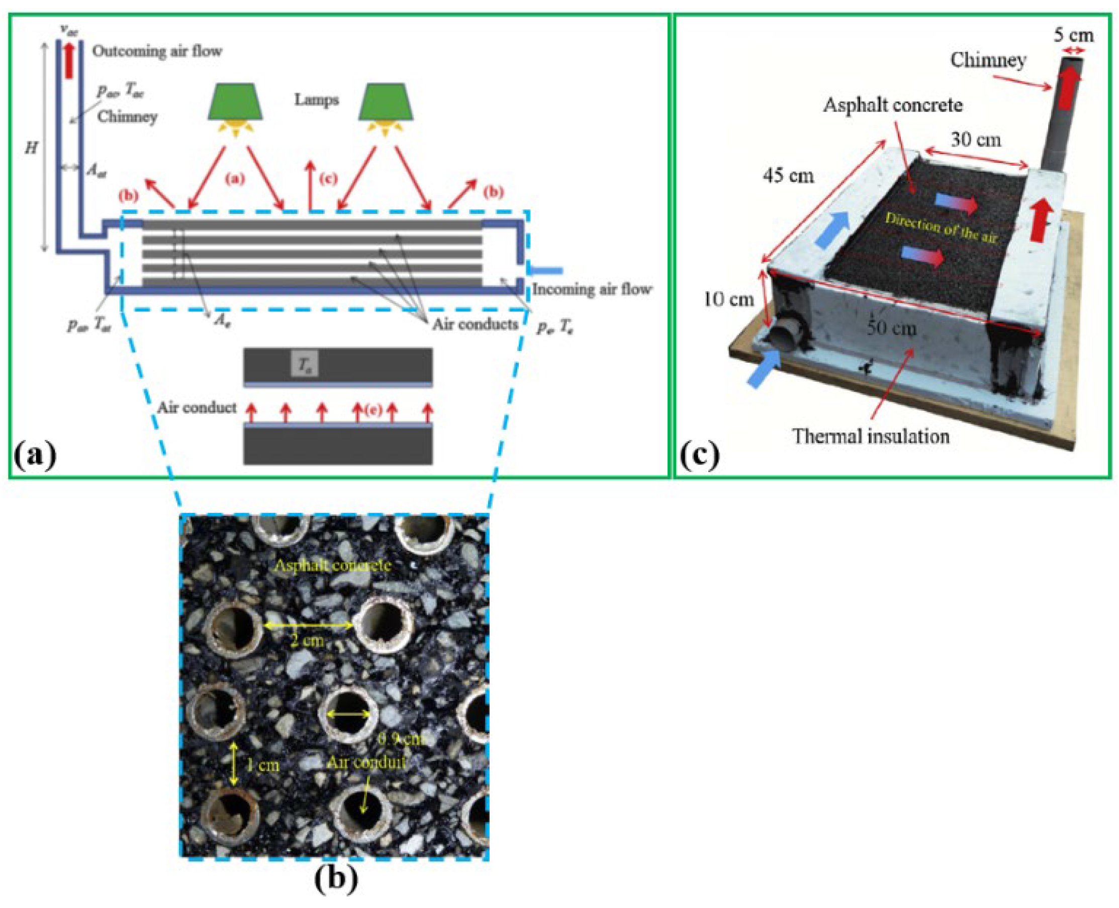
Chiarelli et al. [41,42] conducted a novel testing of the GRES called the ground source heat simulator to investigate the impact of the inlet air temperature and wind speed on system performance. As shown in Figure 30, the dimension of this prototype is 470 × 700 × 180 mm (L × W × H) with a 50 mm thickness of asphalt wearing course and 130 mm of thickness coarse gravel layer; this experiment is carried out at University of Nottingham, UK and divided into two scenarios including air temperature is higher and lower 15 °C of inlet temperature.

Their results reveal from Figure 31a that the most frequent inlet air temperature appears in the range from 14 °C to 15 °C, while the temperatures between 10 °C and 13 °C are also rather frequent; this is because the system is exposed to the outdoor environment, thereby inlet air temperature could not be maintained as a constant value in a real scenario. According to Figure 31b, the wind velocity has a negative effect on the pavement surface temperature; this implies that when the wind is existing, the road surface would be cold and less energy is available for extracting.

Mäkiranta and Hiltunen [43] implemented testing of the GRES to examine the effect of temperature variations at various depths of the soil layer on system energy capturing. As presented in Figure 32, there are four different pipe depths including two for 10 m depth, one for 5 m depth and two for 3 m depth in Finland. Results conclude that it is able to retain appropriate temperature up to 26 °C at the soil depth of 0.5 m, and there are positive temperature values for at least 9 months per annum; this indicates that the soil layer is suitable for assembling heat collection pipes.

Balbay and Esen [44,45] carried out an experimental investigation to explore the feasibility of the GRES utilization to heat roadways for snow melting as shown in Figure 33. During the testing, the processes of snow melting for bridge and pavement slabs at the initial state (t = 0) and intermediate state (t = 30 min.) are shown in Figure 34. Results demonstrate that the top surface of the pavement is typically exposed to bigger temperature fluctuation than the bottom surface. Besides, the thermal conductivity of the concrete slab and air convection coefficient have significant influences on the temperature of the pavement surface; this indicates that the higher wind speed, the higher the convection heat coefficient at the surface of the concrete slab, leading to a lower top surface temperature.

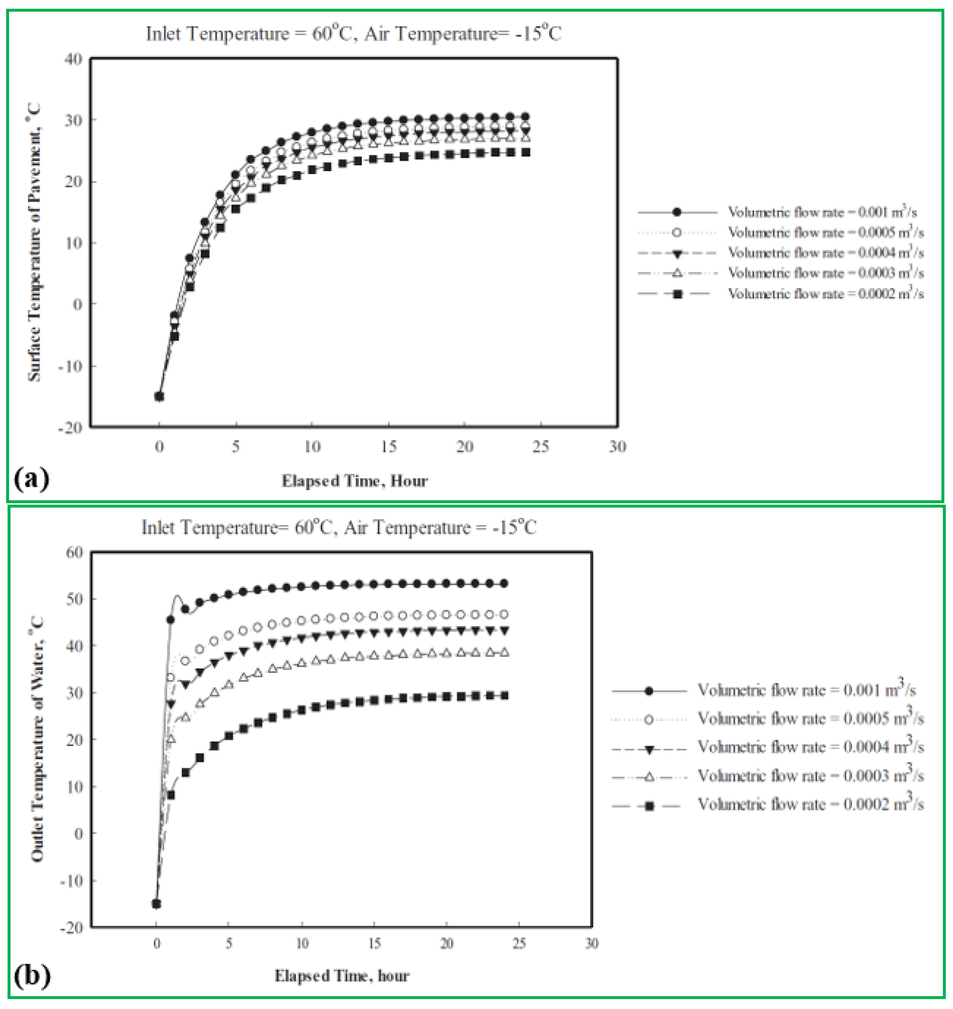
Ho et al. [46] proposed a 3D GRES model to analyze the pavement surface temperature variation. As illustrated in Figure 35, the GRES includes a closed-loop polyethylene tube that is embedded in the concrete slab, and the initial inlet fluid temperature is set in the range of 60 °C to 82.2 °C for snow and ice melting. As shown in Figure 36, a high flow rate can warm road surface to a high temperature, and a low fluid flow rate leads to a big temperature reduction.

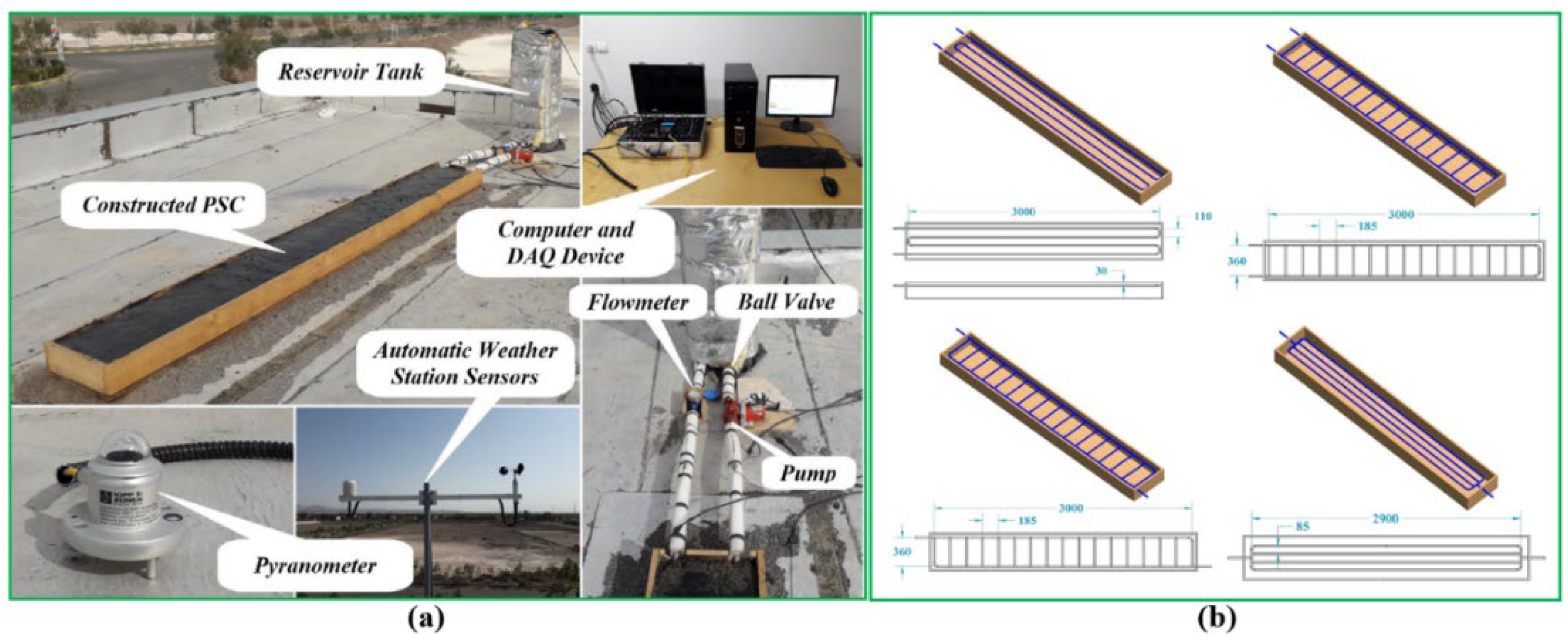
Tota-Maharaj et al. [47] designed a GRES experimental rig to evaluate snow removal rates for various mediums. The GRES consists of a geothermal heat pump (GHP) combined with a permeable pavement system (PPS). Figure 37 despites the interior and exterior views of the testing rig, the interior PPS includes six bins positioned in a temperature-controlled room with an average air temperature of 15 °C, while the exterior part is embedded in the soil where it is subjected to ground temperature and climate conditions. The schematic diagram of the PPS and pavement layers are presented in Figure 38; it is revealed from Figure 39 that the mean snow removal rate varies from 80% to 90% for biochemical oxygen demand (BOD), ammonia–nitrogen (NH4) and orthophosphate–phosphorus (PO4). By comparison, the removal rate of suspended solids (SS) is in the range of 40% to 60%.

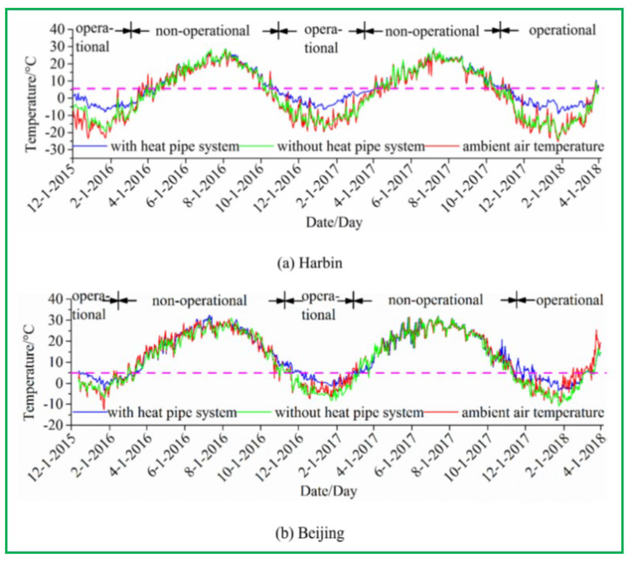
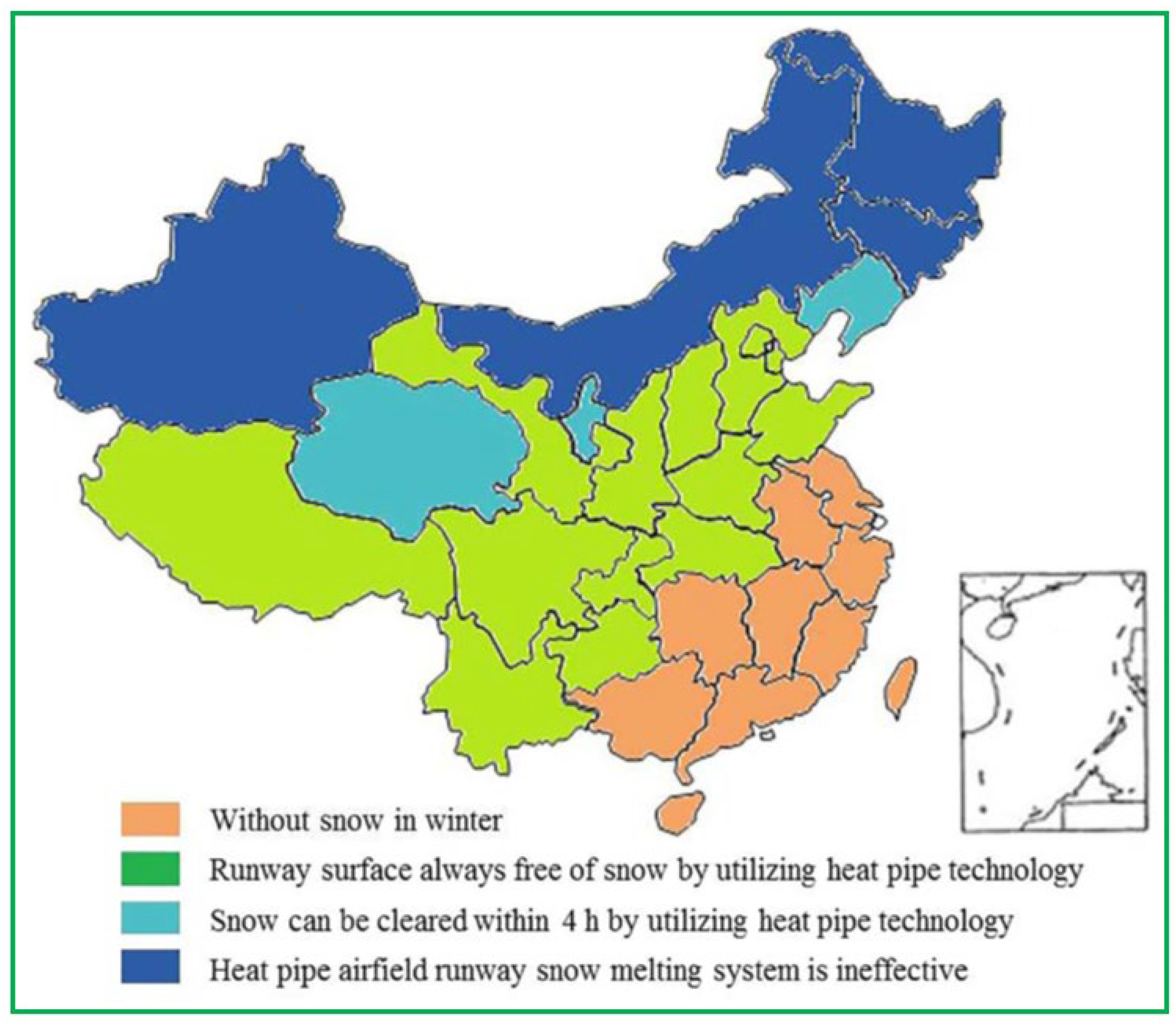
Zhang et al. [48] investigated the snow melting performance of a GRES with L-shaped heat pipe system for airfield runways in Beijing and Harbin of China as depicted in Figure 40; it can be seen from Figure 41 that the GRES could increase the two city mean airfield runway temperatures of 9.1 °C in 2015, 8.9 °C in 2016 and 9.4 °C in 2017, respectively; this implies that the GRES could work automatically primarily in heating season to enhance the surface temperature adequately to avoid ice accumulation; moreover, it can be found that the surface temperature of airfield-runway is below 0 °C at 68% time of the year in Harbin, whereas it is almost above 0 °C in Beijing for the whole winter period; this means that the geography plays a significant role in the system de-icing performance. As shown in Figure 42, the system for airfield-runway is applicable in central areas of China whose air temperature exceeds −10 °C, whereas it is inapplicable in north-western and north-eastern areas.

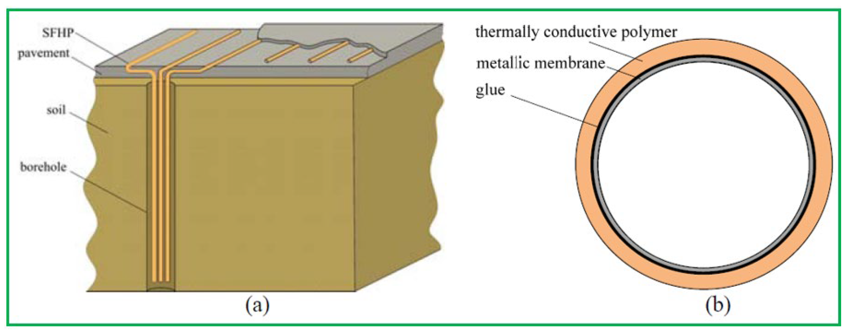
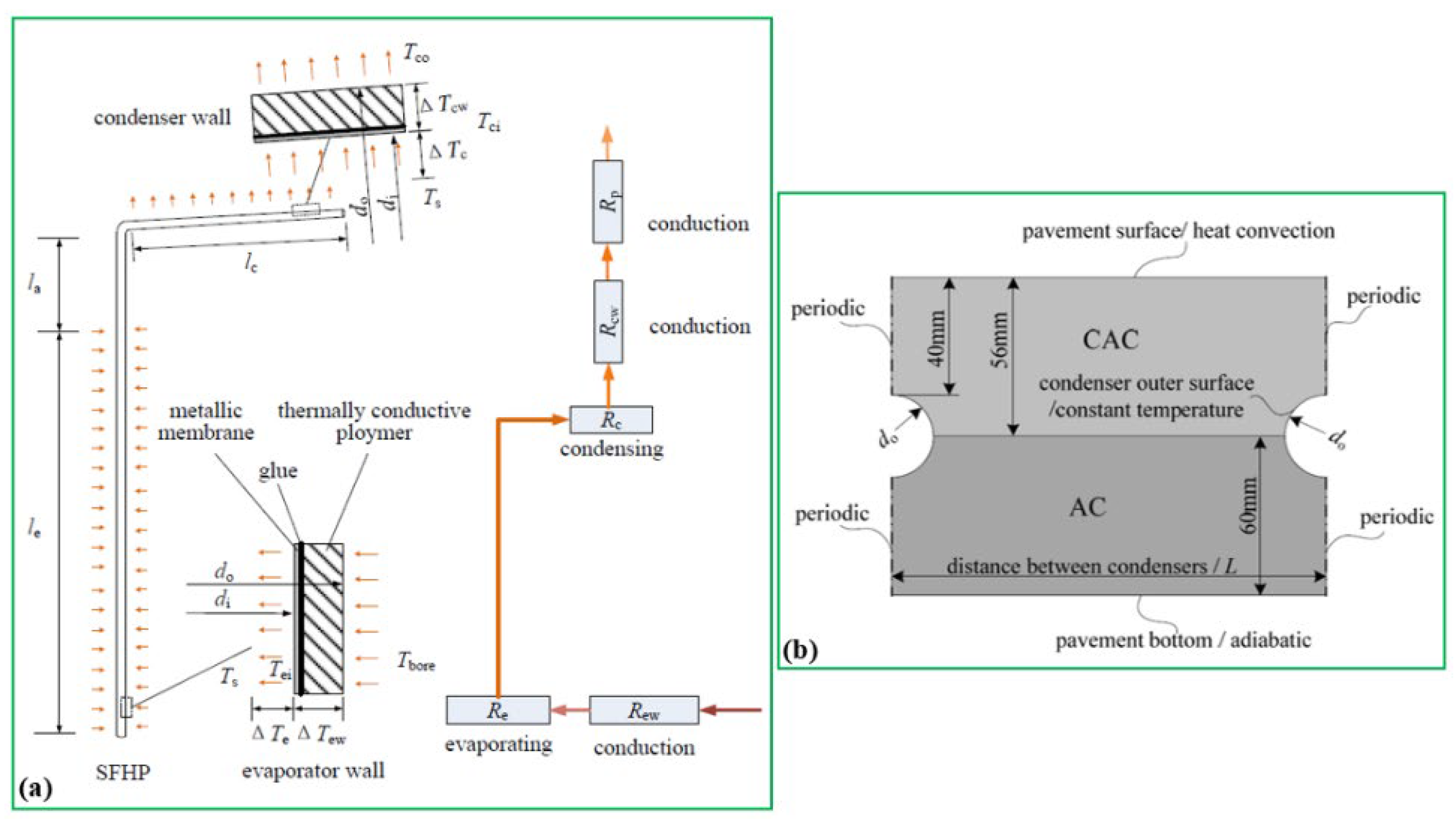
Wang et al. [49] developed a GRES with super flexible heat pipes (SFHPs) system to investigate the entrainment limit within the pipe and provide the optimal design plan based on the local climate condition. The fabrication and construction of the GRES with SFHPs are shown in Figure 43. In order to explore the heat transfer mechanism, thermal resistance model and boundary conditions are given in Figure 44. Simulation results reveal that ammonia is the most suitable thermal fluid for the high entertainment limit, and the system heat output could reach approximately 1.15 kW as illustrated in Figure 45. Besides, 70 m of SFHP length with Ø32 × 2 mm and 0.2 m distance of condenser horizontal interval are recommended as the optimal choice in the study.

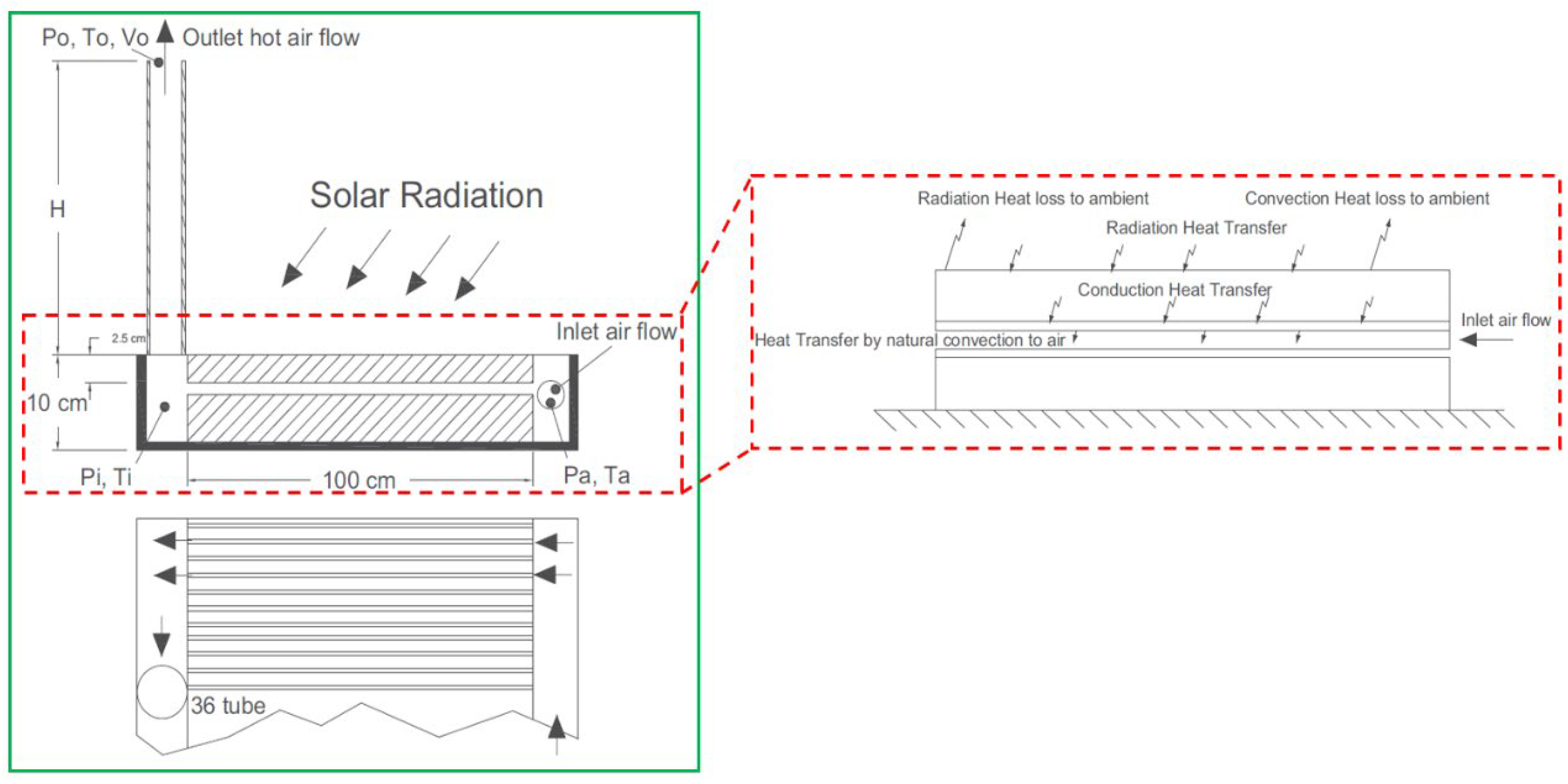
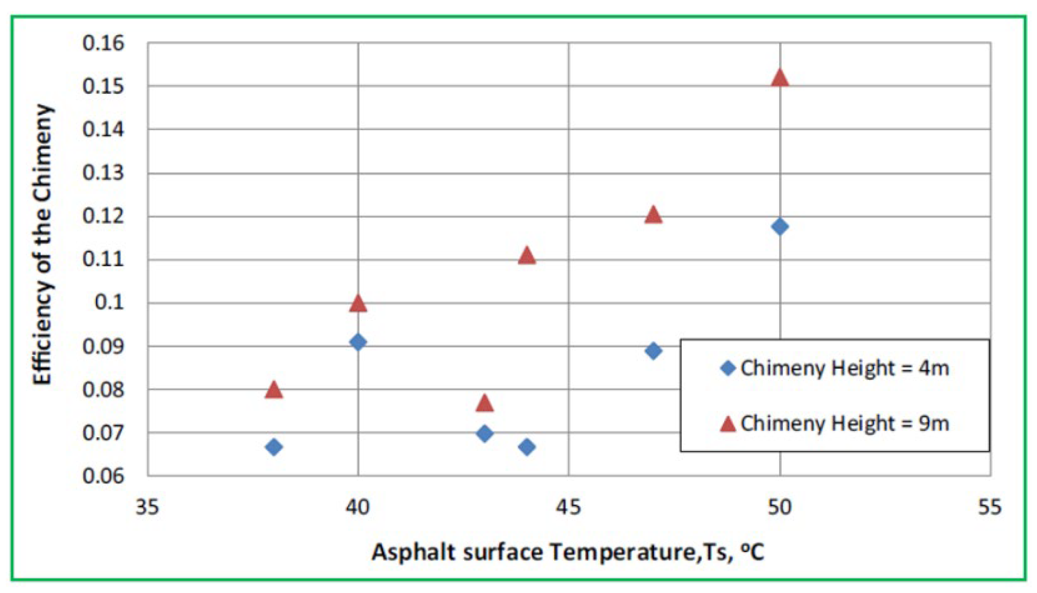
Mauro and Grossman [50] conducted a dynamic GRES simulation work to decrease the fluctuations of street temperature and avert ice formation. The system includes 12 EPs with a diameter of 150 mm and length of 20 m, and the substrate has a thickness of 20 mm and is placed beneath the street pavement with a thickness of 100 mm; it can be found from Figure 46 that the minimum street surface temperature varies from 4.6 °C to 6.6 °C in winter, while the maximum temperature changes from 3.8 °C to 7.5 °C in summer.

3.2. Solar Roadway Energy System

SRES is conducive to mitigating the HIE and eliminating the risk of permanent deformation. Recent studies have aimed to investigate the SRES performance based on experimental analyses and numerical simulations. Hence, some detailed illustrations in terms of roadway surface temperature reduction and influence factors on de-icing and snow melting performance are given in the section. To be more specific, Chiarelli et al. [25] tested an SRES on the basis of different pipe arrangements to evaluate the temperature variation and energy extracted rate. As given in Figure 47, the system involves six 1 m lengths of copper pipes in five configurations, and has two structure layers: a 50 mm thickness of asphalt wearing course layer and a 130 mm thickness of the aggregate layer. Besides, there are six infrared light bulbs that are utilized to heat the surface temperature to 80 °C. Results indicate that the harvested energy is in the range of 60 kJ to 100 kJ whereas their exergy varies from 20 kJ to 40 kJ in six testing periods.

Guldentops et al. [51] setup a 3D COMOSOL model of the SRES to assess the outlet fluid temperature and solar energy absorption efficiency. As shown in Figure 48, the dimension of the calculation region is defined as 4 × 0.9 m (L × W), and the whole length of solar collector pipe is 23.6 m with a diameter of 0.008 m and thickness of 0.3 m.

It can be found from Figure 49a that the system efficiency could be enhanced from 17% to 20% when the thermal conductivity of concrete slab rises from 1.0 to 2.0 W/m·K; this means that a higher thermal conductivity of concrete slab results in more thermal energy obtained by thermal fluid. In comparison, the efficiency of the SRES is increased from 15% to 17% when the absorptivity of the pavement surface is enhanced from 0.65 to 0.95 as depicted in Figure 49b; this indicates that as the asphalt concrete ages, it turns out to be lighter in colour and could, therefore, reflect more of the incident solar radiation. Additionally, the harvested thermal energy reduces from 21% to 14% when the depth of the pipe varies from 25 mm to 105 mm as illustrated in Figure 49c; this indicates that there is a significant influence of the pipe depth on the system performance, meanwhile, the long-time system thermal property enhancement is paramount by reducing the pipe depth as much as possible.

Saad et al. [52] designed an SRES porotype to study the chimney efficiency at different heights. 36 aluminium pipes with a length of 1 m, an interior diameter of 12 mm and a thickness of 0.9 mm are used as given in Figure 50. All pipes are positioned at one level in the horizontal direction placed below 25 mm from the roadway surface slab, and the total thickness of pavement slab is 100 mm. Figure 51 presents the image of the experimental rig; it is found that there is a vital influence of the chimney height on the efficiency. As shown in Figure 52, the chimney efficiency could reach 15% at the chimney height of 9 m whereas the efficiency is 11.7% at the chimney height of 4 m; this implies that the efficiency of the chimney increases with the chimney height.

Johnsson and Adl-Zarrabi [53,54] developed a 3D model of the SRES based on finite difference method (FDM) to study energy usage and de-icing performance. Figure 53 shows that the entire calculation domain of the model is partitioned into segments along z-axial direction, and there are the same thermal properties. By comparison, in the horizontal direction, the model includes several layers with diverse thermal properties. The top of pavement layer is uncovered to the open-air climate, and the boundary condition is defined as the adiabatic or a constant temperature value. The basic heat transfer model is expressed in

Table 5. The 3D model of SRES [53].

Description	Equations
Pavement surface	${\mathrm{q}}_{\mathrm{s}\mathrm{u}\mathrm{r}\mathrm{f}\mathrm{a}\mathrm{c}\mathrm{e}}+{\mathrm{q}}_{\mathrm{conv}}+{\mathrm{q}}_{\mathrm{p}\mathrm{r}\mathrm{e}\mathrm{c}\mathrm{i}\mathrm{p}\mathrm{i}\mathrm{t}\mathrm{a}\mathrm{t}\mathrm{i}\mathrm{o}\mathrm{n}}+{\mathrm{q}}_{\mathrm{l}\mathrm{w}}+{\mathrm{q}}_{\mathrm{s}\mathrm{w}}$ $+{\mathrm{q}}_{\mathrm{e}\mathrm{v}\mathrm{a}\mathrm{p}/\mathrm{c}\mathrm{o}\mathrm{n}}+{\mathrm{q}}_{\mathrm{s}\mathrm{u}\mathrm{b}/\mathrm{d}\mathrm{e}\mathrm{p}\mathrm{o}}+{\mathrm{q}}_{\mathrm{f}\mathrm{r}\mathrm{e}\mathrm{e}\mathrm{z}\mathrm{e}/\mathrm{t}\mathrm{h}\mathrm{a}\mathrm{w}}+{\mathrm{q}}_{\mathrm{t}\mathrm{r}\mathrm{a}\mathrm{f}\mathrm{f}\mathrm{i}\mathrm{c}}=0$
Roadway convection heat flux	${\mathrm{q}}_{\mathrm{conv}}={\mathrm{h}}_{\mathrm{c}}\cdot ({\mathrm{T}}_{\mathrm{a}\mathrm{m}\mathrm{b}\mathrm{i}\mathrm{e}\mathrm{n}\mathrm{t}}-{\mathrm{T}}_{\mathrm{s}\mathrm{u}\mathrm{r}\mathrm{f}\mathrm{a}\mathrm{c}\mathrm{e}})$
Heat flux due to precipitation	${\mathrm{q}}_{\mathrm{p}\mathrm{r}\mathrm{e}\mathrm{c}\mathrm{i}\mathrm{p}\mathrm{i}\mathrm{t}\mathrm{a}\mathrm{t}\mathrm{i}\mathrm{o}\mathrm{n}}={\mathrm{m}}_{\mathrm{p}\mathrm{r}\mathrm{e}\mathrm{c}\mathrm{t}}\cdot {\mathrm{c}}_{\mathrm{p}-\mathrm{p}\mathrm{r}\mathrm{e}\mathrm{c}\mathrm{t}}\cdot ({\mathrm{T}}_{\mathrm{a}\mathrm{m}\mathrm{b}\mathrm{i}\mathrm{e}\mathrm{n}\mathrm{t}}-{\mathrm{T}}_{\mathrm{s}\mathrm{u}\mathrm{r}\mathrm{f}\mathrm{a}\mathrm{c}\mathrm{e}})$
Long-wave radiation	${\mathrm{q}}_{\mathrm{l}\mathrm{w}}={\mathrm{q}}_{\mathrm{l}\mathrm{w}}^{\mathrm{i}\mathrm{n}}-{\mathrm{q}}_{\mathrm{l}\mathrm{w}}^{\mathrm{o}\mathrm{u}\mathrm{t}}$ ${\mathrm{q}}_{\mathrm{l}\mathrm{w}}^{\mathrm{i}\mathrm{n}}={\mathrm{F}}_{\mathrm{s}\mathrm{k}\mathrm{y}\mathrm{v}\mathrm{i}\mathrm{e}\mathrm{w}}{\mathsf{\epsilon }}_{\mathrm{s}\mathrm{k}\mathrm{y}}\mathsf{\sigma }{\mathrm{T}}_{\mathrm{a}\mathrm{m}\mathrm{b}\mathrm{i}\mathrm{e}\mathrm{n}\mathrm{t}}^4+(1-{\mathrm{F}}_{\mathrm{s}\mathrm{k}\mathrm{y}\mathrm{v}\mathrm{i}\mathrm{e}\mathrm{w}})\mathsf{\sigma }{\mathrm{T}}_{\mathrm{a}\mathrm{m}\mathrm{b}\mathrm{i}\mathrm{e}\mathrm{n}\mathrm{t}}^4$ ${\mathrm{q}}_{\mathrm{l}\mathrm{w}}^{\mathrm{o}\mathrm{u}\mathrm{t}}={\mathsf{\epsilon }}_{\mathrm{s}\mathrm{u}\mathrm{r}\mathrm{f}\mathrm{a}\mathrm{c}\mathrm{e}}\mathsf{\sigma }{\mathrm{T}}_{\mathrm{s}\mathrm{u}\mathrm{r}\mathrm{f}\mathrm{a}\mathrm{c}\mathrm{e}}^4$
Short-wave radiation	${\mathrm{q}}_{\mathrm{s}\mathrm{w}}=(1-{\mathsf{\alpha }}_1)\cdot \mathrm{I}$
Sensible heat from the traffic	${\mathrm{q}}_{\mathrm{t}\mathrm{r}\mathrm{a}\mathrm{f}\mathrm{f}\mathrm{i}\mathrm{c}}=0$
Fluid temperature reduction in each segment	${\mathrm{T}}_{\mathrm{f}}^{\mathrm{k}}={\mathrm{T}}_0^{\mathrm{k}}+({\mathrm{T}}_{\mathrm{f}}^{\mathrm{k}-1}-{\mathrm{T}}_0^{\mathrm{k}}){\mathrm{e}}^{-\mathrm{L}\mathrm{s}\mathrm{e}\mathrm{g}/\mathrm{l}\mathrm{c}}$ ${\mathrm{T}}_0^{\mathrm{k}}=2{\mathrm{R}}_0(\frac{{\mathrm{T}}_{\mathrm{i},\mathrm{j}}^{\mathrm{k}}}{{\mathrm{R}}_{\mathrm{i},\mathrm{j}}^{\mathrm{p}\mathrm{i}\mathrm{p}\mathrm{e}}}+\frac{{\mathrm{T}}_{\mathrm{i},\mathrm{j}+1}^{\mathrm{k}}}{{\mathrm{R}}_{\mathrm{i},\mathrm{j}+1}^{\mathrm{p}\mathrm{i}\mathrm{p}\mathrm{e}}})$ ${\mathrm{R}}_0={[2(\frac{1}{{\mathrm{R}}_{\mathrm{i},\mathrm{j}}^{\mathrm{p}\mathrm{i}\mathrm{p}\mathrm{e}}}+\frac{1}{{\mathrm{R}}_{\mathrm{i},\mathrm{j}+1}^{\mathrm{p}\mathrm{i}\mathrm{p}\mathrm{e}}})]}^{-1}$
Heat flux from one segment	${\mathrm{q}}_{\mathrm{f}}^{\mathrm{k}}=\frac{({\mathsf{\nu }}_{\mathrm{f}}\mathsf{\pi }{\mathrm{r}}_{\mathrm{p}\mathrm{i}}^2)\cdot {\mathsf{\rho }}_{\mathrm{f}}\cdot {\mathrm{c}}_{\mathrm{f}}({\mathrm{T}}_{\mathrm{f}}^{\mathrm{k}-1}-{\mathrm{T}}_{\mathrm{f}}^{\mathrm{k}})}{{\mathrm{L}}_{\mathrm{s}\mathrm{e}\mathrm{g}}}$
Heat flux nearby the pipe	${\mathrm{q}}_{\mathrm{i},\mathrm{j}}^{{\mathrm{k}}^{\mathrm{s}\mathrm{o}\mathrm{u}\mathrm{r}\mathrm{c}\mathrm{e}}}={\mathrm{q}}_{\mathrm{f}}^{\mathrm{k}}\frac{{\mathrm{R}}_0}{{\mathrm{R}}_{\mathrm{i},\mathrm{j}}^{\mathrm{p}\mathrm{i}\mathrm{p}\mathrm{e}}}+\frac{{\mathrm{T}}_0^{\mathrm{k}}-{\mathrm{T}}_{\mathrm{i},\mathrm{j}}^{\mathrm{k}}}{{\mathrm{R}}_{\mathrm{i},\mathrm{j}}^{\mathrm{p}\mathrm{i}\mathrm{p}\mathrm{e}}}$

.

As shown in Figure 54, a top layer of pavement slab involves the polyethylene pipe is positioned at a depth of 62 mm with a distance of 50 mm, 10 parallel pipes within the concrete have a length of around 140 m and cover an area of 70 m². A good agreement in terms of surface temperature between the testing and numerical results is achieved as illustrated in Figure 55, the root mean square error (RMSE) and mean error (ME) are 1.34 °C and −0.55 °C, respectively. As illustrated in Figure 56, the energy usage varies from 330 kWh/m² to 540 kWh/m² with an ice and snow cover lasting for 1100 h to 430 h, respectively; this implies that about 62% of system energy consumption could be saved by using the SRES.

Zaim et al. [55] implemented a testing investigation of the SRES to analyse the influence of pipe configuration on the system performance as depicted in Figure 57a. Specifically, the system composes of pipe loops, a tank, a water pump, a flowmeter, a pyranometer, an anemometer and a data logger. The pipe external dimension is 3 × 0.4 × 0.2 m (L × W × H) with the inner diameter of 15.8 mm, which is embedded in a regular arrangement with a center-to-center spacing of around 110 mm; furthermore, Figure 57b presents various configurations involving the parallel, series, balanced and unbalanced ladder-shape that are constructed in the SRES; it can be found from Figure 58 that the pipe arrangements have significantly effects on the system outlet fluid temperature during the testing. The outlet fluid temperatures are similar between the balanced ladder-shape and parallel arrangements, but the highest outlet fluid temperature occurs in the series pipe arrangement. As demonstrated in Figure 59, the various pipe arrangements have little influence on the pavement surface temperature; however, solar irradiation plays a vital role in the surface temperature.

Alonso-Estébanez et al. [56] built a 3D CFD model of the SRES to assess the influences of solar radiation and different slab thickness on system performance. As shown in Figure 60, the numerical model consists of four calculation regions involving working fluid within the pipe, copper pipe, asphalt mixture and ambient air. The boundaries of the top and side walls within the ambient air domain are 20 m away from the heat source. The water velocity and flow rate are defined as 1.6 m/s and 2 L/min, respectively. Meanwhile, an experimental test is implemented to validate the 3D model as presented in Figure 61. The prototype consists of a 2 × 2 configuration that includes 4 slabs with 420 × 130 × 60 mm (L × W × D) and a U-tube copper pipe with exterior and interior diameters of 1.7 m and 0.016 m and a depth of 0.25 m. The validation result confirms that the errors between numerical and experimental results do not exceed 10% in terms of thermal performance, temperature variation and energy collection. As demonstrated in Figure 62a, solar radiation has important influences on the pavement surface temperature, working fluid flow rate and size, the system thermal efficiency could reach up to 74% based on the simulation analysis. What is more, the additional energy stored within the roadway slabs has less impact on system thermal performance as illustrated in Figure 62b.

Daniels et al. [57] designed a prototype of the SRES to assess de-icing performance in the USA. As illustrated in Figure 63, the testing slab has a dimension of 3050 × 1220 × 130 mm (L × W × D), and a 500-gallon thermal storage tank is used to link the pavement slabs and solar collectors, and placed on a high density polyurethane foam as its bottom insulation. The polyethylene pipe is embedded below the pavement surface of 50 mm to meet the minimum concrete cover demand. As shown in Figure 64, an infrared image of the snow-melting process of pavement surface is given in the period of 6 h from 4:37 a.m. to 10:37 a.m. After the SRES works about 4.13 h, the power consumption is around 0.51 kWh, thereby, the fluid temperature of the thermal storage tank could decrease from 60 °C to 49.4 °C during the test period.

García and Partl [58] conducted an experimental study of the SRES with parallel air conduits to overcome the damage of the buried pipes and evaluate the system efficiency. As shown in Figure 65, sixty steel tubes with 300 mm length and internal and external diameters of 9 and 11 mm are embedded in the asphalt concrete material. Two air chambers of 10 × 10 × 45 cm are assembled at both sides of the test porotype as the inlet and outlet of the air conduits. Results from Figure 66 reveal that system efficiencies could be improved around 10% and 12% for heating up air and chimney usage, respectively, implying that it is extreme important to use the chimney.

Wu et al. [59] explored the influences of fluid flow rate within the SRES on the pavement surface and the heat obtained. As described in Figure 67, the prototype composes of a small-scale asphalt solar collector, a circulation pump, a flow meter and a control valve. The pavement slab includes three layers of compacted asphalt mixture that has a dimension of 300 × 300 × 150 mm (L × W × D). The hose pipe is regarded as thermal isolation and utilized to connect all devices. Results from Figure 68a demonstrate that the working flow rate has a restricted effect on the maximum surface temperature. In particular, when the working flow rate increases to 1886 mL/min, the surface temperature decreases up to 36.7 °C, by comparison, when the working flow rate falls to 54 mL/min, the temperature reaches the maximum value of 38.58 °C; this indicates that the high working fluid rate results in a superior amount of thermal energy that could be extracted. Additionally, it can be observed from Figure 68b that thermal energy of about 400 W/m² can be extracted when the flow rate is in the range of 400 to 1800 mL/min; this means that the flow rate has less influence on enhancing the heat transfer coefficient of working fluid within the pipe.

Du et al. [60] established a new numerical model to analyze the temperature distribution and heat transfer rate in comparison with the control structure. As illustrated in Figure 69a, the calculation domain includes asphalt layers that have a base and sub-base layers with a size of 5 × 5 cm, subgrade and steel rods that have dimensions of 5 × 10 cm and 0.6 × 2 cm, respectively. The model boundary conditions for top, left and right are defined as thermally insulated and constant thermal properties of all materials. Besides, the temperatures and heat fluxes of sections A, B and C are employed to study the model heat transfer mechanism as presented in Figure 69b. Seven rod-implanting modes are applied to investigate their effects on the temperature distribution for the pavement as exhibited in Figure 69c. The simulation results in Figure 70a reveal that the new model could absorb about 31% solar energy in comparison with the control structure; furthermore, the internal and surface temperatures could be decreased by up to 6.4 °C and 3.5 °C, respectively, in comparison to the control structure, as exhibited in Figure 70b.

Dakessian et al. [61] compared two SRES efficiencies between a close-loop configuration and a single-pass configuration as displayed in Figure 71, and found that the single-pass system could reach the efficiency of 21.9% while the close-loop system achieves the efficiency of 10.9%. Additionally, as shown in Figure 72, a 3D finite element model of the SRES is established to investigate the energy harvesting and roadways surface temperature variations for the single-pass system at different seasons; it is demonstrated from Figure 73 that the single-pass SRES could enhance water temperature and decrease roadways surface temperature by 10.2 °C and 1.24 °C for spring, 13.6 °C and 1.69 °C for summer, 7.5 °C and 0.67 °C for autumn as well as 4 °C and 0.52 °C for winter, respectively.

3.3. Summary

To sum up, both the GRES and SRES use renewable energy technologies to solve the problems induced by conventional chemical-based snow and ice melting approaches. The two types have the ability to decrease energy consumption by approximately 30%, and increase the surface temperature of roadway by around 5 °C in winter and reduce it by 6 °C in summer.

Table 6. Detailed descripted of GRES.

Researchers	Type	Region	Method	Working Fluid	Key Findings
Liu et al. [26,27]	Hybrid horizontal and vertical	Canada	Numerical model	Water	The energy consumption could be decreased by 29% through using insulation materials. About 30% growth in the snowfall rate could cause around a 35% increasing of energy consumption. The flow fluid rate within the GRES has the most vital influence on spiral loops. Soil thermal imbalance not only disturbs system energy efficiency but also badly affects the structural integrity of EP.
Yu et al. [28]	Horizontal	USA	Experiment testing	Water	The system could provide about 60% heating to the surface of the bridge deck. The heat flux of the surface obtained from the GRES is in the range from 120 to 270 W/m2.
Fabrice et al. [30]	Vertical	Switzerland	Numerical model	Water	The thermally induced stresses have a vital effect on the short-term local temperature gradient and pile temperature. The average overstress could achieve 80 kPa/°C and 90 kPa/°C for cooling and heating seasons, respectively
Kong et al. [31]	Horizontal	China	Experiment testing	Water	The thermal expansion strain variation is linearly with the increment of concrete slab temperature. The maximum stress caused by the GRES is lower than design parameter.
Mirzanamadi et al. [32,33,34]	Horizontal	Sweden	Numerical model and experiment testing	Ethylene glycol-water solution	The system performance could be improved based on the closer distance between each pipe, the shallow depth, big pipe diameter and low emissivity parameter of the pavement surface. The most vital effect on enhancing system de-icing performance is the distance between each pipe to shorten the hours of slippery. There are 2% drop in the capturing solar energy and 5% fall in the needed energy for de-icing performance when the working fluid rate is in the range between 8 L/min and 50 L/min.
Adl-Zarrabi et al. [35]	Horizontal	Sweden	Numerical model	Water	The system performance is based on pipes arrangement, thermal properties of concrete slab as well as temperature level of the thermal storage unit. The distance between the pipes has a bigger effect on the system thermal performance compared with the pipe buried depth.
Xu et al. [36]	Horizontal	China	Numerical model and experiment testing	Ethylene glycol-water solution	The heat mass GRES model contributes to averting overestimating the requirement of the heat flux to obtain the most optimum system. In comparison with the heat-only GRES model, the needed heat fluxes could be decreased ranging from 6% to 17% through the heat-mass model.
Han and Yu [37,38]	Vertical	USA	Numerical model	Ethylene glycol-water solution	The spiral shaped pipe could extract more heat compared with other shapes. The growth of working fluid velocity has few effects on the soil energy obtained for the U- and W- shapes whereas it has a vital influence on the spiral-shape. The GRES with PCM model could extract more soil heat energy and cut down the requirement of pile number for de-icing pavement surface.
Ho and Dickson [39]	Horizontal	USA	Numerical model	Ethylene glycol-water solution	The GRES is suggested to install the soil layer that has a high degree of saturation and high thermal conductivity. The most optimum volumetric flow rate is recommended as at or beneath 1.0 L/s.
Yang et al. [40]	Horizontal	China	Numerical model	Ethylene glycol-water solution	The GRES applied in the underground tunnel has an important influence on energy-saving and producing more cooling. Lower inlet fluid temperature and flow velocity conduce to enhancing the heat exchange efficiency.
Chiarelli et al. [41,42]	Horizontal	UK	Numerical model and experiment testing	Water	Simulation results reveal that surface pavement temperature could improve from 0.4 °C and 2.1 °C in winter by comparison, the temperature could reduce 2 °C–6 °C in summer. The pavement temperature in winter depends upon the air temperature and humidity.
Mäkiranta and Hiltunen [43]	Vertical	Finland	Experiment testing	Ethylene glycol-water solution	Soil temperature at depth of 0.5 m is very promising for heat extraction during cooling season in Finland. Asphalt heat could be regarded as thermal energy storage, and decrease the peak loads of heat energy consumption in winter.
Balbay and Esen [44,45]	Vertical	Turkey	Numerical model and experiment testing	Propylene glycol	Results conclude that the top surface temperatures of pavement and bridge exhibit more fluctuations compared with the bottom one. Air convection coefficient and thermal conductivity of BS and PS have an important influence on surface temperature. The system COP could achieve 1.99 for 30 m soil depth, 2.66 for 60 m soil depth and 3.05 for 90 m soil depth, respectively.
Ho et al. [46]	Horizontal	USA	Numerical model	Water	It can be found that when 60 °C of working fluid temperature to de-icing the road surface, it is applicable to most the weather conditions in the USA. When air temperature varies from −5 °C to −25 °C and working fluid could achieve between 50 °C and 60 °C, the GRES is able to operate well, by contrast, when the working fluid ranges from 30 °C and 40 °C, the GRES could not operate efficiently.
Tota-Maharaj et al. [47]	Vertical	UK	Experiment testing	Water	The mean removal rates vary between 80 and 90% for BOD, NH4 and PO4. By comparison, the removal rate of suspended solids (SS) is in the range from 40% and 60%. The system EER efficiency could attain ranging from 1.5 to 2.5.
Zhang et al. [48]	Horizontal	China	Experiment testing	Ethylene glycol-water solution	The GRES could work automatically largely in the heating season and enhance the surface pavement temperature. The geography has a critical effect on the system de-icing performance. The GRES could enhance the road surface temperature by about 17 °C. The GRES technology could be utilized in more than 78% of the cities in China.
Wang et al. [49]	Vertical	China	Numerical model	Ammonia	The system heat output could achieve approximately 1.15 kW. The suggested entire length of SFHPs is 70 m with Ø 32 × 2 mm and 0.2 m distance of condenser horizontal interval.
Mauro and Grossman [50]	Vertical	Italy	Numerical model	Ethylene glycol-water solution	The system could enhance the street surface temperature ranging from 4.6 °C to 6.6 °C in heating season. The system could decrease the street surface temperature ranging from 3.8 °C to 7.5 °C in cooling season.

and

Table 7. Detailed description of SRES.

Researchers	Type	Region	Method	Working Fluid	Key Findings
Chiarelli et al. [25]	Vertical	Finland	Experiment testing	Atmospheric air	The energy harvested could reach ranging from 60 kJ and 100 kJ whereas their exergy varies from 20 kJ and 40 kJ during the six testing period. The roadway surface temperature can be reduced by up to 5.5 °C.
Guldentops et al. [51]	Horizontal	USA	Numerical model and experiment testing	Atmospheric air	Thermal production is increased from 14% to 21% when the depth of pipe is decreased from 105 mm to 25 mm. The system efficiency rises from 17% to 20% when the thermal conductivity of the concrete slab enhances, ranging between 1.0 and 2.0 W/m·K. The increase in thermal behavior and decrease of the pipe depth are significant for system’s long-term operation.
Saad et al. [52]	Hybrid horizontal and vertical	Canada	Numerical model	Atmospheric air	The chimney efficiency based on different heights has an important influence on the pavement surface temperature. The chimney efficiency could achieve 15% and 11.7% for 9 m and 4 m height chimney, respectively.
Johnsson and Adl-Zarrabi [53,54]	Horizontal	USA	Experiment testing	Ethylene glycol-water solution	The ME between testing and numerical results is approximately −0.55 °C while the RMSE is about 1.39 °C. The system could decrease the energy consumption by 62%. The average surface roadway temperature could be reduced about 6.4 °C in summer.
Zaim et al. [55]	Horizontal	Sweden	Numerical model and experiment testing	Water	The various pipe arrangements have few influence on the roadway surface temperature under different seasons. The system indicates that the solar irradiation plays a vital effect on the roadway surface temperature. The growing of solar radiation contributes to booting the average surface temperature.
Alonso-Estébanez et al. [56]	Horizontal	Sweden	Numerical model	Water	The system could achieve 74% of thermal efficiency. The thickness of the collector has a little influence on the thermal performance.
Daniels et al. [57]	Horizontal	China	Numerical model and experiment testing	Ethylene glycol-water solution	The power consumption is around 0.51 kWh when the SRES works about 4.13 h. The fluid temperature of thermal storage tank could decrease from 60 °C to 49.4 °C during the test period.
García and Partl [58]	Vertical	USA	Numerical model	Atmospheric air	The system efficiency could reach around 10% and 12% for heating up air and chimney usage, respectively, It is extreme vital to decrease the energy loss by the chimney.
Wu et al. [59]	Horizontal	UK	Numerical model and experiment testing	Water	The surface temperature reduces up to 36.7 °C, when the working flow rate enhances to 1886 mL/min. The surface temperature could achieve up to 38.58 °C, when the working flow rate decreases to 54 mL/min. The growth of flow rate conduces to boosting the heat transfer coefficient of fluid inside the pipe.
Du et al. [60]	Vertical	Turkey	Numerical model and experiment testing	Water	The model could absorb about 31% solar energy in comparison with the control structure. The internal and surface temperatures could decrease by up to 6.4 °C and 3.5 °C, respectively, in comparison to the control structure.
Dakessian et al. [61]	Horizontal	Lebanon	Numerical model and experiment testing	Water	The single-pass system could reach an efficiency of 21.9% which is higher compared with the close-loop system reaching 10.9%. The single-pass SRES could enhance water temperature and decrease roadways surface temperature by an average of 10.2 °C and 1.24 °C for spring, 13.6 °C and 1.69 °C for summer, 7.5 °C and 0.67 °C for autumn as well as 4 °C and 0.52 °C for winter, respectively.

illustrate the research regions, applied methods and key findings. What is more, the effects of climate condition, pipe type and dimension, pipe arrangement, flow rate, initial fluid temperature, thermal conductivities of soil and wearing layer, absorptivity and emissivity of the roadway surface, preheating time, chimney height, slab thickness and pavement surface absorptivity, on the GRES and SRES de-icing and snow melting performance are individually summarized and compared in

Table 8. The influences of various parameters on GRES performance.

System	Researchers	Impact Factors
		Climate Condition	Pipe Arrangement Type	Pile Diameter and Depth	Distance between Pipe	Evaporator Section Length	Flow Rate	Initial Fluid Temperature	Thermal Conductivity of Wearing Layer	Thermal Conductivity of Soil	Emissivity of Road Surface	Absorptivity of Road Surface	Thermal Recharging Analysis	Preheating Time
GRES	Liu et al. [26,27]	✓	✖	✓	✖	✖	✓	✓	✖	✖	✖	✖	✓	✖
	Yu et al. [28,29]	✓	✖	✓	✓	✖	✖	✖	✖	✖	✖	✖	✖	✖
	Fabrice et al. [30]	✓	✖	✓	✓	✖	✓	✓	✖	✖	✖	✖	✖	✖
	Kong et al. [31]	✓	✖	✖	✖	✖	✖	✓	✖	✖	✖	✖	✖	✖
	Mirzanamadi et al. [32,33,34]	✓	✖	✓	✓	✖	✓	✓	✓	✓	✓	✓	✖	✖
	Adl-Zarrabi et al. [35]	✓	✖	✓	✓	✖	✓	✓	✖	✓	✖	✖	✖	✓
	Xu et al. [36]	✓	✖	✖	✖	✖	✖	✖	✖	✖	✖	✖	✖	✓
	Han and Yu [37,38]	✓	✓	✖	✖	✖	✖	✖	✖	✖	✖	✖	✖	✖
	Ho and Dickson [39]	✓	✖	✓	✓	✖	✓	✓	✖	✓	✖	✖	✖	✖
	Yang et al. [40]	✖	✖	✖	✖	✖	✓	✖	✖	✖	✖	✖	✖	✖
	Chiarelli et al. [41,42]	✓	✖	✖	✖	✖	✖	✖	✖	✖	✖	✖	✖	✖
	Mäkiranta and Hiltunen [43]	✓	✖	✓	✖	✖	✖	✖	✖	✓	✖	✖	✖	✖
	Balbay and Esen [44,45]	✖	✖	✓	✖	✖	✖	✖	✖	✖	✖	✖	✖	✖
	Ho et al. [46]	✓	✖	✖	✖	✖	✓	✓	✖	✖	✖	✖	✖	✖
	Tota-Maharaj et al. [47]	✓	✖	✖	✖	✖	✖	✖	✖	✖	✖	✖	✖	✖
	Zhang et al. [48]	✓	✖	✓	✓	✓	✖	✖	✖	✖	✖	✖	✖	✖
	Wang et al. [49]	✖	✖	✖	✓	✖	✖	✓	✖	✖	✖	✖	✖	✖
	Mauro and Grossman [50]	✓	✖	✖	✖	✖	✖	✖	✖	✖	✖	✖	✖	✖

and

Table 9. The effects of different parameters on SRES performance.

System	Researchers	Impact Factors
		Climate Conditions	Pipe Arrangement Type	Pile Diameter	Pipe Depth	Distance between Pipe	Chimney Height	Chimney Inlet Temperature	Air Flow Rate	Fluid Flow Rate	Slab Thickness	Wind Speed	Thermal Conductivity of Slab Concrete	Pavement Surface Absorptivity
SRES	Chiarelli et al. [25]	✓	✓	✓	✖	✓	✖	✖	✓	✖	✖	✖	✖	✖
	Guldentops et al. [51]	✖	✖	✖	✓	✖	✖	✖	✖	✖	✖	✖	✓	✓
	Saad et al. [52]	✖	✖	✖	✖	✖	✓	✓	✓	✖	✖	✓	✖	✖
	Johnsson and Adl-Zarrabi [53,54]	✓	✖	✖	✖	✓	✖	✖	✖	✓	✖	✖	✖	✖
	Zaim et al. [55]	✓	✓	✖	✖	✖	✖	✖	✖	✖	✖	✓	✖	✖
	Alonso-Estébanez et al. [56]	✖	✖	✓	✖	✖	✖	✖	✖	✓	✓	✖	✖	✖
	Daniels et al. [57]	✓	✖	✖	✖	✖	✖	✖	✖	✖	✖	✓	✖	✖
	García and Partl [58]	✖	✖	✖	✖	✖	✓	✓	✓	✖	✖	✖	✖	✖
	Wu et al. [59]	✖	✖	✖	✓	✖	✖	✖	✖	✓	✖	✖	✖	✖
	Du et al. [60]	✓	✖	✓	✓	✓	✖	✖	✖	✖	✖	✖	✖	✖
	Dakessian et al. [61]	✓	✖	✖	✓	✖	✖	✖	✖	✖	✖	✖	✖	✖

; it is discovered that the climate condition, pipe layout arrangements, soil thermal conductivity, preheating time, slab thickness and chimney height play a significant role in the GRES and SRES performance whereas the diameter of pipe has a slight influence.

4. Economic Assessment

Various economic feasibility researches are implemented to determine the cost-savings of the GRES and SRES as well as their payback periods (PBP). Typically, the capital investments of the GRES and SRES primarily involve project design, heat pump unit and installation; moreover, the system operating costs include power consumption of heat pump, monitoring, maintenance and replacement. Hence, some key models and cases are elaborated in the section.

4.1. Geothermal Roadway Energy Systems

Liu et al. [27] carried out an economic analysis of the GRES with the EP in order to determine the cost-saving and PBP in Canada. As illustrated in Figure 74, it can be found that the PBP of the GRES is less than 4 years compared with the traditional electrical heating unit’s; furthermore, the GRES has the potential to save about CAD 1.5 million by the end of 30 years’ operating.

Han and Yu [38] conducted an economic assessment for a modified GRES with PCM to assess the expense factor and decrease the expense barrier. In this study, the additional expenses of five PCM categories are investigated as depicted in Figure 75; it is found that the system expense of cyclohexane is more than ten times higher compared with the other materials’. Meanwhile, when an EP with 3% PCM is used to replace the cyclohexane, a 90% system cost-saving can be achieved; this indicates that when the expense of materials decreases, the expense barriers are able to be removed. The additional expense of the EP could be decreased to USD 207 when the biodiesel crude glycerine is used in the model. Yang et al. [40] implemented a finical evaluation of the GRES to resolve the high capital investment and assess the system financial viability in a typical city of China. Results obtained from Figure 76 reflect that the total net present value (NPV) could be 150,000 CNY when the internal rate of return (IRR) is 4.9% for 15-year’s operating period. In the meantime, the system PBP is approximately 8 years. Mauro and Grossman [50] analysed how to decrease the cost of the GRES based on pipe configuration. In this study, the main expenses of the whole system include the pipe material purchasing, rock-soil drilling, installation, customized concrete attained through using high thermal conductivity aggregates and the mixture preparation; it is found that the cost of the GRES is in the range between 850 and 1250 EUR/m², however, it is possible to be further cut to about 450 EUR/m² by materials optimization, size modified and hollow pile installation.

Habibzadeh-Bigdarvish et al. [62] performed life cycle cost (LCC) and sensitive analyses of the GRES for bridge deck de-icing based on the Monte Carlo Simulation (MSC) method. Results from Figure 77a reveal that the main cash flow is from traffic flow improvement profits in the 25th and 32nd years of the analysis; this means that the traffic flow improvement is the most sensitive random variable. Meanwhile, the NPV value indicates that the system profits overweigh its initial investment after 25 years, and could achieve USD 2.4 million after 50 years. According to Figure 77b, the GRES is a cost effective solution for heating bridge deck when the daily traffic volume is over a minimum of 7000 vehicles.

Nahvi et al. [63] conducted economic analyses of the GRES for the Minneapolis/Saint Paul International Airport (MSP) and Des Moines International Airport (DSM). Results from Figure 78a show that the annual system energy consumption costs at the MSP could reach about USD 1.96 million which is almost six times higher compared to that at the DSM; moreover, as shown in Figure 78b, the benefit-cost ratio (BCR) is the most sensitive to capital investment on the basis of the dimension of airport and site location. In other words, the numbers of airplane operating have a significant influence on the BCR.

4.2. Solar Roadway Assessment Energy Systems

Dakessian L et al. [61] carried out an economic investigation for the SRES in the light of the life extension, NPV and PBP based on a 10 m section of a two-lane road in Lebanon. As indicated in Figure 79, the SRES could extend the lifetime service from 20 to 23 years, thus saving the cost of about USD 600 compared with the conventional roadway. Furthermore, a positive NPV of USD 3000 with about 5 years of the PBP is achieved in the study.

Sable [64] implemented a finical assessment of the SRES to investigate the system payback period and cost-saving; it is found that the annual cost-saving could be achieved in the range of Rs. 6106.5 to Rs. 9838.3, in the meantime, the PBP is in the range from 2.3 to 4.1 years.

4.3. Summary

Several economic models are utilized broadly to study the economic factors affecting the markets for the GRES and SRES in various countries and regions. Based on the research results, the GRES has a higher capital investment because of the drilling and installation fees, which are almost three times higher than those of the SRES, while the PBPs of the GRES and SRES are in the ranges of 4 to 8 years and 2.3 to 5 years respectively. A detailed summary of economic analyses of the GRES and SRES by different researchers is shown in

Table 10. Economic analyses of GRES and SRES.

Researchers	Type	Region	Key Findings
Liu et al. [27]	GRES	Canada	For geothermal EP system, the initial excavation expense can be saved in comparison with the traditional geothermal heat pump system. The PBP for the GRES is less than 4 years than the traditional electrical heating system. The GRES is able to save about CAD 1.5 million by the end of 30 years’ operating.
Han and Yu [38]	GRES	USA	The system expense of cyclohexane is ten times higher compared with the other materials. A 90% system cost-saving could be achieved when an EP with at 3% PCM is replaced via the cyclohexane. When the expense of materials is dropped, the expense barriers are able to be removed.
Yang et al. [40]	GRES	China	The total NPV could achieve CNY 150,000 when the internal rate of return (IRR) is 4.9% during the 15-year’s operating period. The system PBP is approximately 8 years.
Mauro and Grossman [50]	GRES	Italy	The system cost is able to be further cut to about 450 EUR/m2 by materials optimization, size modified and hollow piles application.
Habibzadeh-Bigdarvish [62]	GRES	USA	The cash flow is from traffic flow improvement benefits in the 25th and 32nd years of the assessment. The NPV presents that the benefits of system overweigh its initial investigation after 25 years, and could achieve USD 2.4 million after 50 years. The system could provide a cost effective solution for heating bridges decks when the daily traffic volume could achieve a minimum of 7000 vehicles.
Nahvi et al. [63]	GRES	USA	The annual system energy consumption costs at MSP could reach about USD 1.96 million which is nearly 6 times bigger than that at DSM reaching around USD 0.34 million. The BCR is the most sensitive to capital investment on the basis of the dimensions of airport. The numbers of airplane operating have a significant influence on the BCR.
Dakessian et al. [61]	SRES	Lebanon	The SRES could extend the lifetime service from 20 to 23 years, thus saving the cost of about USD 600 compared with the conventional roadway. A positive NPV of USD 3000 with about 5 years of PBP are achieved for the system.
Sable [64]	SRES	India	The annual cost-saving could achieve ranging between Rs. 6106.5 and Rs. 9838.3. The PBP is in the range from 2.3 to 4.1 years.

. In addition, there is often an extraordinary discrepancy in the financial influence factors, including initial cost, operation and maintenance expenses and inflation rates, operations and delay periods as well as percentage of weather related delay, which could cause considerable differences in the investment decision and key financial performance, as presented in

Table 11. The economic influence factors of GRES and SRES.

Researchers	Types	Regions	Influence Factors
			Initial Investment	Discounted Rate	Inflation Rate	Internal Rate of Return	Maintenance and Operation Cost	Number of Operations and Delay Durations	Percentage of Weather Related Delay
Liu et al. [27]	GRES	Canada	✓	✖	✓	✖	✓	✖	✖
Han and Yu [38]	GRES	USA	✓	✖	✖	✖	✓	✖	✖
Yang et al. [40]	GRES	China	✓	✖	✖	✓	✓	✖	✖
Mauro and Grossman [50]	GRES	Italy	✓	✖	✖	✖	✓	✖	✖
Habibzadeh-Bigdarvish [62]	GRES	USA	✓	✓	✖	✖	✓	✖	✖
Nahvi et al. [63]	GRES	USA	✓	✓	✖	✖	✓	✓	✓
Dakessian et al. [61]	SRES	Lebanon	✓	✖	✖	✖	✓	✓	✖
Sable [64]	SRES	India	✓	✖	✓	✖	✓	✖	✖

.

5. Future Developments

The GRES and SRES as renewable energy systems are imperatively challenging areas of research in terms of climate condition, pipe configuration and material, thermal conductivities of soil and slab concrete, and initial design condition. Although more endeavours have been focused on the advanced and promising techniques, there are still a few challenges needed to be disposed for forthcoming exploration and spreading out the applicability of the technologies, those challenges are displayed as below:

• Numerical models of the GRES and SRES are still required to be established to predict the system de-icing and snow-melting performance more accurately, thereby this contributes to improving system designs in the future.
• Further investigation on the GRES and SRES should be focused on the construction and maintenance technique for pavement with pipes; this is because if the subsidence deformation or structure crack happens during the fitting and operation, this may damage the enclosed state, causing the groundwater entry and pipeline leak, and decreasing the system service lifetime. Hence, it is essential to setup a real time monitoring system to check the effect of the surrounding environment on the structure deformation.
• Heat pipe is generally banded with the reinforced steel cage in the EP system, therefore massive attention should be spent to avoid the pipe damage during concreting, and appropriate measures should be adopted to prevent blockage at the connecting point. What is more, freezing injury should be taken into account in cold region, this is because the frozen soil and road excavation may result in the freezing of water within the GRSE. Furthermore, using the PCM to replace the regular concrete in ground heat exchanger should be further studied.
• The soil and asphalt layers can store thermal energy in the GRES, therefore, in this aspect, the thermal storage capacity should be clarified to complement roadway energy consumption.
• A detail analysis should be implemented to identify the influences of air convection on the physical properties of the GRES and SRES in the fields of energy capturing, LCC and CO₂ emission.

6. Conclusions

The GRES and SRES can effectively solve ice and snow accumulation issues on roadway which cause inconvenience for drivers and traffic accidents in winter, but they consume less energy and produce less or no CO₂ emission compared with conventional chemical based melting solutions. In summer, the GRES and SRES can reduce the pavement surface temperature to mitigate the heat effect and extend its service lifetime. A comprehensive review of their technological performance and economic evaluation is conducted in this study based on numerical and economic models, and experimental analyses. Three vital aspects of the technology performance assessment, involving roadway surface temperature, energy consumption and main influence factors, are explored in different regions and countries. Energy and economic evaluations of the two technologies for various climatic conditions, different pipe configurations and design conditions are carried out as well. As a result, some crucial conclusions are summarized as follow:

• The climate data such as ambient temperature, solar radiation, snowfall rate as well as wind speed, are the essential information to design de-icing and snow-melting systems.
• The spiral shape pipe could extract more soil heat in comparison with U-shape and W-shape pipes, so it is the best choice in the GRES system under the limited pile length. The velocity of the working fluid has less effects on the system performance with the U- and W- shape pipes whereas it has a significant influence on that with the spiral-shape pipe.
• Approximately 35% less hours of the pavement slippery condition are achieved when the working fluid temperature increases by about 15 °C in the GRES.
• In the GRES, the soil thermal imbalance influences not only the system energy conversion but also the structural foundation, so this imbalance should be avoided by injecting a large amount of heat to the soil.
• The modified GRES, such as using the EP and PCM to replace the traditional ground pipe loop and concrete, could extract more thermal energy and reduce the pile number for de-icing pavement surface, which is conducive to decreasing the capital investment and maintenance cost.
• In the SRES, the increasing of the pipe thermal conductivity and decreasing of its depth have significant effects on the system long-term operation. The thermal gain decreases from 21% to 14% when the depth of the ground pipe varies from 25 mm to 105 mm.
• In the SRES, the chimney height is a vital parameter influencing on the system performance, the chimney efficiency increases from 11.7% to 15% when its height rise from 4 m to 9 m. The higher the chimney, the lower the energy loss.
• Compared with the traditional ways, the GRES and SRES could decrease energy consumption by approximately 30%, the roadway surface temperature could be increased by around 5 °C in winter and reduced by about 6 °C in summer.
• The service lifetimes of the GRES and SRES could attain 25 to 30 years and 20 to 23 years, respectively. The GRES has a higher capital investment because of the drilling and installation fees, which is almost three times higher than that of the SRES, while the PBPs of the GRES and SRES are in the ranges of 4 to 8 years and 2.3 to 5 years respectively.