Article

Land-Use-Based Runoff Yield Method to Modify Hydrological Model for Flood Management: A Case in the Basin of Simple Underlying Surface

College of Urban and Environmental Sciences, Peking University, No.5 Yiheyuan Road, Haidian District, Beijing 100871, China
*
Author to whom correspondence should be addressed.
Sustainability 2022, 14(17), 10895; https://doi.org/10.3390/su141710895
Submission received: 5 August 2022 / Revised: 26 August 2022 / Accepted: 28 August 2022 / Published: 31 August 2022
(This article belongs to the Special Issue Regional Climate Change and Application of Remote Sensing)

Abstract

:
The study of runoff under the influence of human activities is a research hot spot in the field of water science. Land-use change is one of the main forms of human activities and it is also the major driver of changes to the runoff process. As for the relationship between land use and the runoff process, runoff yield theories pointed out that the runoff yield capacity is spatially heterogeneous. The present work hypothesizes that the distribution of the runoff yield can be divided by land use, which is, areas with the same land-use type are similar in runoff yield, while areas of different land uses are significantly different. To prove it, we proposed a land-use-based framework for runoff yield calculations based on a conceptual rainfall–runoff model, the Xin’anjiang (XAJ) model. Based on the framework, the modified land-use-based Xin’anjiang (L-XAJ) model was constructed by replacing the yielding area (f/F) in the water storage capacity curve of the XAJ model with the area ratio of different land-use types (L/F; L is the area of specific land-use types, F is the whole basin area). The L-XAJ model was then applied to the typical cultivated–urban binary land-use-type basin (Taipingchi basin) to evaluate its performance. Results showed great success of the L-XAJ model, which demonstrated the area ratio of different land-use types can represent the corresponding yielding area in the XAJ model. The L-XAJ model enhanced the physical meaning of the runoff generation in the XAJ model and was expected to be used in the sustainable development of basin water resources.

1. Introduction

The sustainable development of water resources has intimate associations with the quality of human life in modern society [1,2,3]. A runoff yield calculation is one of the key components in basin water resource management, which plays an important role in hydrologic processes [4,5,6,7,8]. In the past few decades, runoff yield models, which were used for hydrological forecasting and water resources management, have been providing decision-making services for basin management and planning [5,9,10,11,12,13]. Saturation-excess runoff generation theory pointed out that runoff occurs when the soil water content in the unsaturated zone exceeds the field capacity [14]. Based on this theory, numerous rainfall–runoff models have been developed and applied extensively around the world over the past century, which proved the effectiveness of the theory [15,16,17,18,19].
The runoff yield is closely related to the underlying surface condition [20,21]. In a basin, the characteristics of runoff yield are spatially differentiated. Different hydrological models invariably construct a curve to describe this difference in the runoff yield, e.g., the water storage capacity curve of the XAJ model, which has demonstrated widespread utility in most natural basins of humid and semi-humid regions [22,23]. However, intensive human activities are changing the natural basin deeply [24], which has a profound impact on the runoff yield. The natural distribution of the runoff yield and the original runoff yield mechanism are changed along with these drastic land-use changes [25,26,27]. Zhu et al. [28] and Zheng et al. [29] have found that land-use change is the strongest contributor to a change in the runoff process and may be directly responsible for more than 70%. Studies also found that hydrological models tend to underperform more in artificial basins than in natural basins [25]. Some scholars pointed out that it is mainly due to the land-use changes, which influence the runoff yield [30,31,32].
The effect of land use on the runoff yield was widely discussed in hydrology [33,34,35]. The basic consensus is that land-use change is the most important factor affecting the runoff yield [24,36,37,38,39,40,41,42,43,44]. Among them, lots of studies concentrated on the relationship between different land-use changes and runoff yield (e.g., vegetation [45,46,47,48], urbanization [49,50], agricultural activities [51,52,53]). In general, afforestation will reduce the runoff yield, while deforestation, urbanization and overgrazing will increase the runoff yield; furthermore, the effect of agricultural activities varies with tillage practices [54,55,56,57,58,59]. Moreover, relevant studies indicated that the land-use structure and spatial layout (e.g., land-use distribution [60,61], land-use pattern and landscape features [62,63]) also have a deep impact on the runoff yield, runoff patterns and the runoff processes. These studies suggest that the land-use type is closely related to the runoff processes, which may be the key factor to determine the runoff yield.
Although many studies concerned the relationship between land-use change and runoff [64,65,66], few of them took land use as a parameter to integrate into conceptual hydrological models. Inspired by previous scholars, this paper assumes that the distribution of the runoff yield can be divided by the land-use form, i.e., areas with the same land-use form are similar in their runoff yield, while areas of different land uses are significantly different. As for the XAJ model, it can be expressed by replacing the yielding area with the area ratio of land use in the basin. The main objective of this study is to construct a land-use-based Xin’anjiang (L-XAJ) model with the relationship between the yielding area (f/F) and the area of different land uses (L/F) for better runoff generation simulation in a typical cultivated–urban binary land-use-type basin, thus providing a better tool for the sustainable development of water resources at the basin scale. This research is expected to be used for flood management and the sustainable development of water resources in the basin. The remainder of this paper was organized as follows: Section 2 describes the methods and study area, Section 3 summarizes the research results and discussions and, lastly, the conclusions are drawn in Section 4.

2. Materials and Methods

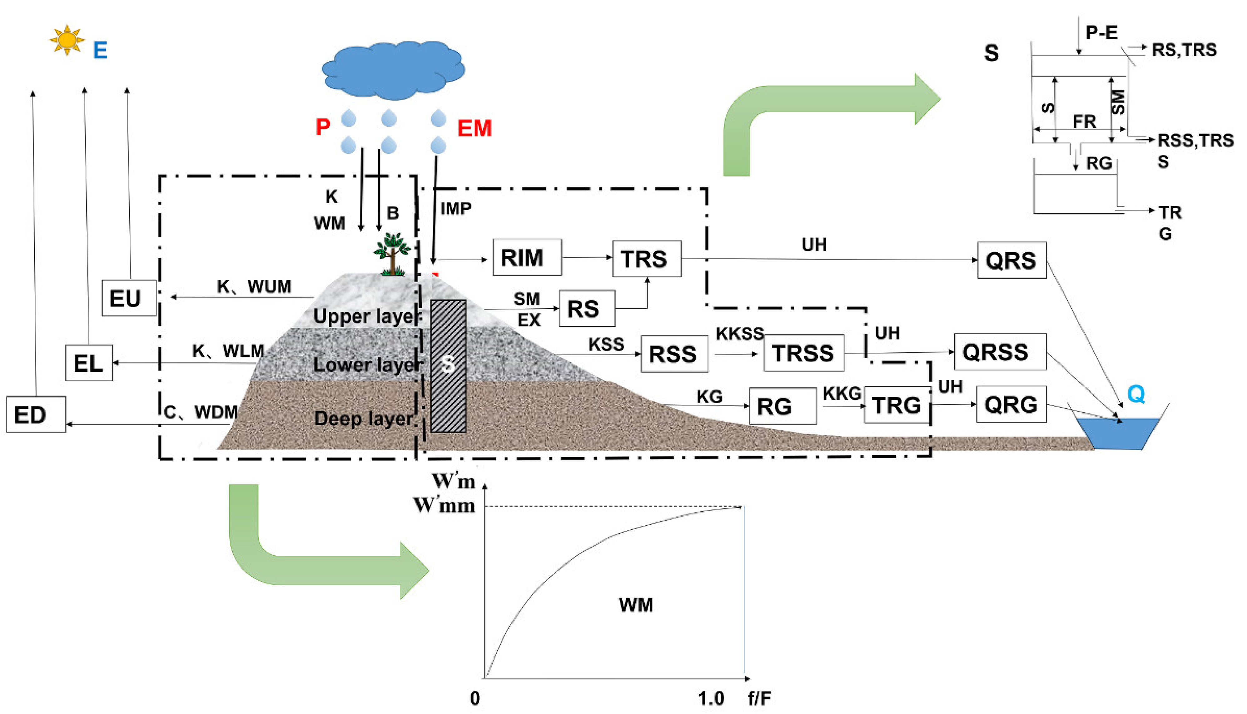
2.1. Runoff Yield in XAJ Model

XAJ model is one of the most famous hydrological models in China, which is widely used in humid and semi-humid areas [14]. XAJ model can be divided into four parts: evapotranspiration, runoff generation, runoff sources partition and runoff concentration (Figure 1). Runoff generation is one of the most important modules and the parabolic curve is used to calculate the runoff yield, which can be represented by the following equation:
f F = 1     ( 1     W m W mm ) B
where W m is the storage capacity of a point in the basin (mm), f is the fraction of the basin area for which the storage capacity is less than W m , F is the whole basin area, W mm is the maximum value of W m and B is the shape parameter of the storage capacity distribution.
Based on Equation (1), the average water storage capacity (WM) of the basin can be obtained:
WM = 0 1 W m d ( f F ) = W mm 1 + B
As shown in Figure 2a, there are two basic initial assumptions for the runoff generation process: (1) the initial soil water content of the basin is W 0   and the maximum field storage capacity is A; (2) the area of a proportion of α 0   over the basin is in saturation state and the rainfall that falls on this area directly produces runoff, on the area of 1 − α 0   , it does not. Hence, the initial state of the basin is:
A = W mm * [ 1     ( 1     W 0   WM ) 1 1 + B ]
If rainfall is P and evapotranspiration is E, when evapotranspiration exceeds rainfall (P − E < 0), runoff is not generated; when rainfall exceeds evapotranspiration (P − E > 0), then runoff is generated.
If P − E + A < W mm for local runoff generation, the soil water storage is the LOSS part in Figure 2a and the runoff yield R can be obtained by the following equation:
R = dPE     A A + ( P     E ) ( 1     α 0 ) dW m   = P     E + WM ( 1     A + P     E W mm ) B + 1 + W 0       WM
Otherwise, the runoff yield R can be obtained by the equation:
R = P         E       ( WM       W 0 )
The runoff generation process can be calculated by Equations (4) and (5). From Equations (4) and (5), the rainfall–runoff relationship can be obtained as Figure 2b, which indicates that runoff yield only is controlled by net rainfall P-E and soil moisture W 0   .

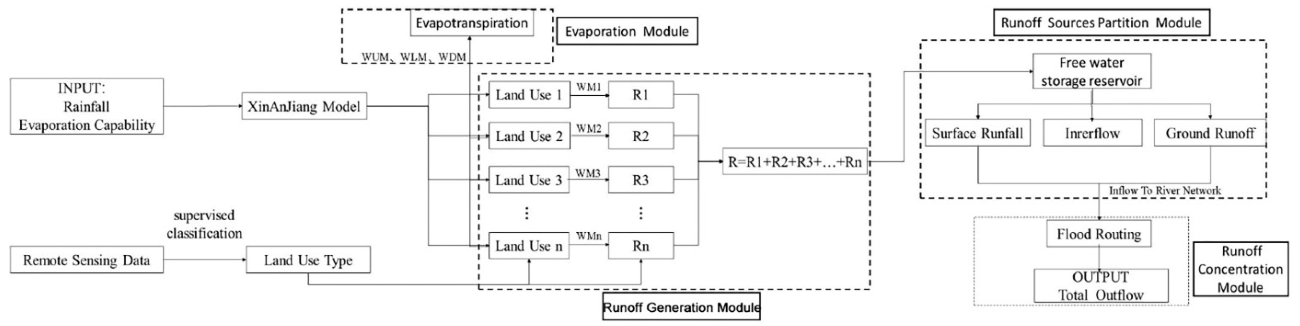
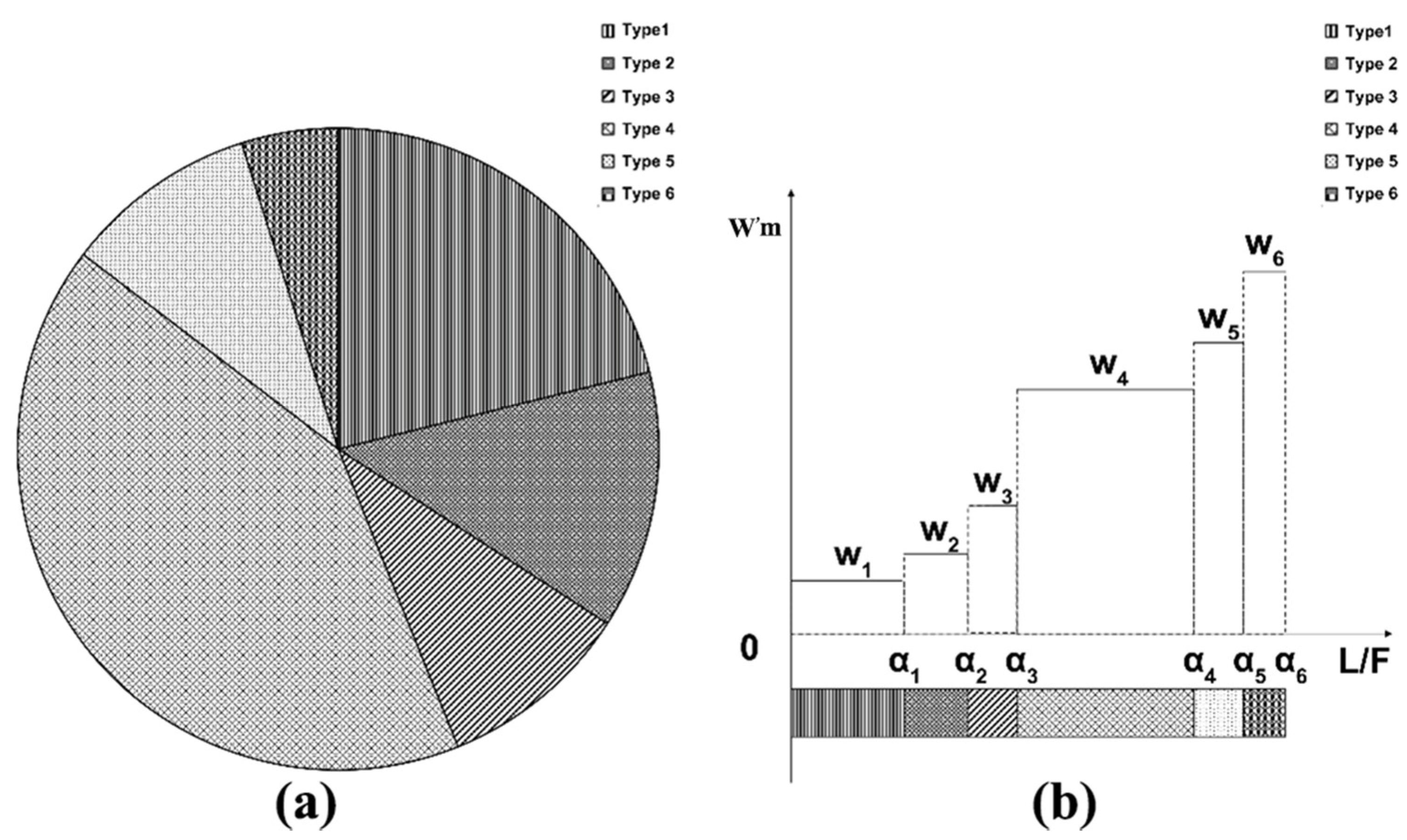
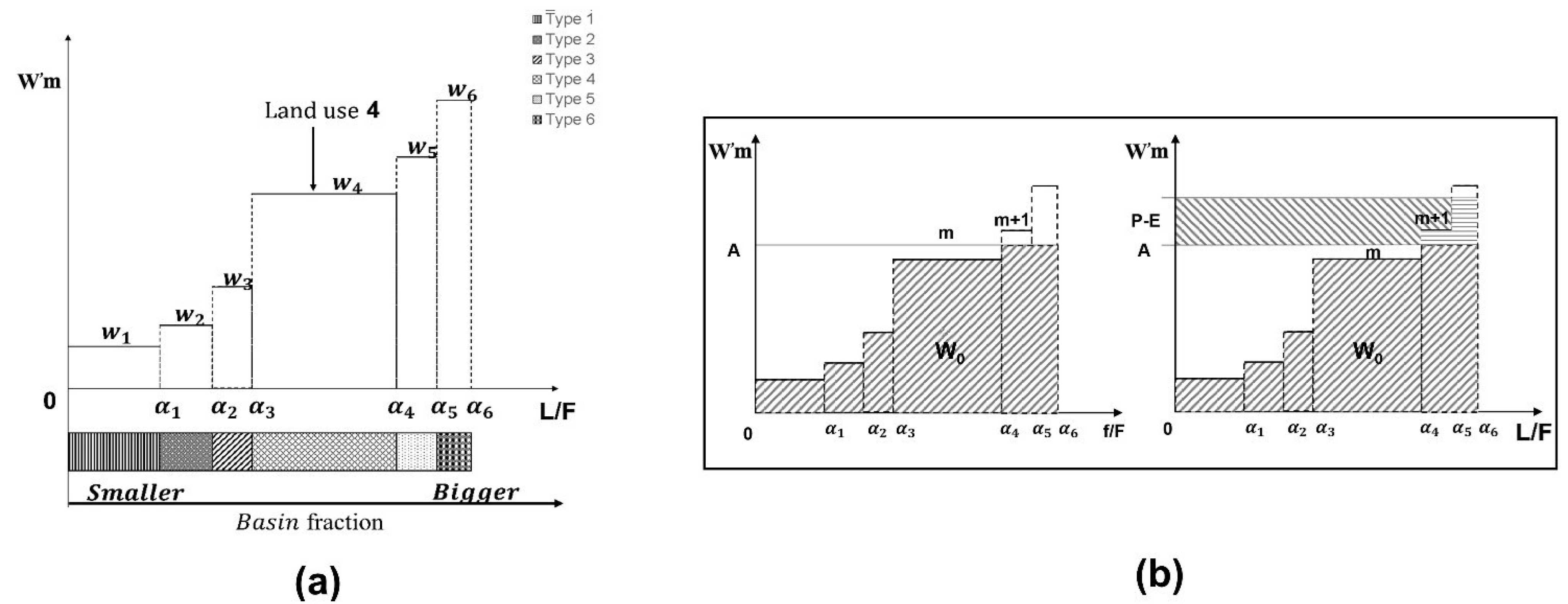
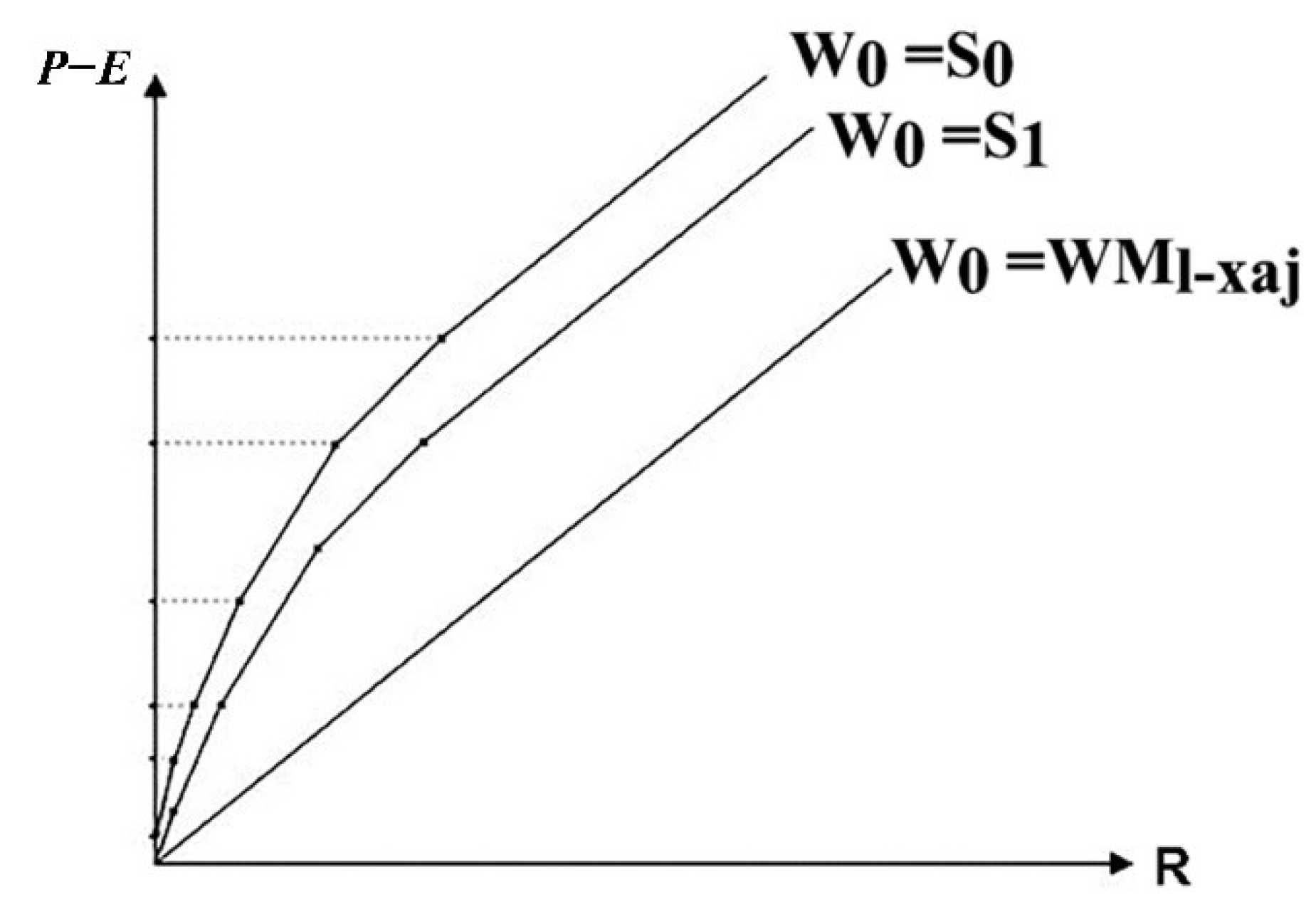
2.2. Runoff Yield in L-XAJ Model

The XAJ model provides an effective solution for runoff yield calculation but has no clear physical meaning [67,68]. However, its parameters implicitly represent the influence of underlying surface factors such as land use on runoff yield. To clarify the underlying surface information of the model, we assumed that the distribution of runoff yield in a basin can be divided by land-use form, i.e., areas with the same land-use form are similar in runoff yield, while areas of different land uses are significantly different. L-XAJ model calculates the runoff yield under each land-use type by specific water storage capacity value, accumulates the runoff yield of all land-use types as the basin’s runoff yield and then goes into the free water storage reservoir for the partition of runoff sources (Figure 3).
As shown in Figure 4, land-use pattern can be obtained from remote sensing images. This is assuming that the land use of the rectangle can be divided into four regions, A, B, C and D, which is grassland, forest, urban and grassland, respectively. Though the water storage capacity is spatially heterogeneous in this rectangle, it can be roughly distinguished as the four regions. The water storage capacity values of regions A and D, are roughly at the same level; while the values of regions A, B and C are at different levels. So, we can use a mean value a to represent the average water storage capacity of region A and D, a mean value b for region B and a mean value c for region C; a, b and c are not equal to each other.
In this framework, water storage capacity is indeed different at different points within the same land-use type. It is difficult to calculate the water storage capacity of each point, but its statistical law is presented in the water storage capacity curve of XAJ model. The mean value of each land-use segment is used to represent its water storage capacity value.
To describe the land-use-based water storage capacity curve by clear mathematical formulas, we assume that there are n different land-use types in a certain basin (Figure 5a) and their area ratios over the basin are s 1 ,   s 2 s n , respectively, as the abscissa in L-XAJ model by αi, such as (α0, α1], (α1, α2] …(αn−1, αn], where α0 = 0, αi − αi−1 = si (1 ≤ i ≤ n) (Figure 5b). The water storage capacity value of different land-use types are W1, W2 …Wn, representing the average value of the water storage capacity of different land-use types as the ordinate in L-XAJ model. As shown in Figure 6a, L-XAJ model is a monotone increasing piecewise function and each segment of the function represents one kind of land-use type in the basin, including urban, surface water bodies, grassland, crops, forest, etc. In application, land-use types can be adjusted based on the true condition of different basins. The area of i-th (1 ≤ i ≤ n) land-use type is αi − αi−1 = si and was reflected on the abscissa in L-XAJ model. The water storage capacity value of the ith land-use type is Wi, reflecting the ordinate in L-XAJ model, and the water storage capacity value within [αi−1, αi] is always Wi. Therefore, the average water storage capacity of the ith land-use type WS i can be obtained:
WS i = W i × ( α i     α i 1 ) = W i × s i   ( 1     i     n )
In addition, the average storage capacity, WM l xaj , of L-XAJ model can be calculated as follows:
WM l xaj = i = 1 n WS i = i = 1 n W i × ( α i     α i 1 )   ( 1 i n )
In the quantification, the shape of the L-XAJ model is determined by certain constraints. In this paper, the total water storage capacity of the same basin should be the same. Therefore, there are two constraints of XAJ model and L-XAJ model: (1) the maximum water storage capacity of the basin should be the same and (2) the average water storage capacity also should be the same. So:
WM = W mm 1 + B = WM l xaj = i = 1 n W i × ( α i     α i 1 )
Additionally,
W mm = W n
Here, W mm and B are the parameters of XAJ model, which can be obtained by parameter calibration, n and α i are the land-use parameters, which can be obtained from the land-use analysis of the basin, W i is the water storage capacity value of ith land-use type and W n is the maximum water storage capacity value.
After the L-XAJ model is constructed, it is necessary to further analyze the rainfall–runoff relationship and calculate the runoff yield under different rainfall conditions. As shown in Figure 6b, we assume that the basin soil moisture before rainfall is W 0 , which is distributed horizontally in L-XAJ model, the first m land-use types in the basin have reached the saturation state, while the m + 1 land-use type has not reached or has just reached it. In this case:
A = W 0     i = 1 m W i × ( α i     α i 1 ) 1     α m
If rainfall is P, evapotranspiration is E. When evapotranspiration exceeds rainfall (P − E < 0), runoff is not generated. When rainfall exceeds evapotranspiration (P − E > 0) then, if P − E + A > Wn, total runoff generation:
R = P     E     ( WM l xaj     W 0 )
Otherwise, for local runoff generation, the soil water storage is the horizontal fill part in Figure 6b and runoff yield R is:
R = ( P     E )     i = a b ( W i     A ) · ( α i     α i 1 )     i = b + 1 n ( P     E ) · ( α i     α i 1 )
where a and b satisfy the constraints:
W a > A P     E + A W b
where a takes the smallest integer value that satisfies Equation (13) and b takes the largest integer value.
So, the runoff yield of L-XAJ model can be calculated by Equations (11) and (12) and the rainfall–runoff interactions can be studied. When set, the soil moisture content is Si (S0 = 0) and at the same time, the soil moisture is just enough to make the land-use type i reach the storage-full state. In this condition, the rainfall–runoff relationship (Figure 7) is different to XAJ model; it is segmented form, but there is continuity between adjacent segments. When W 0 = S0, the line is n segments with different slopes, which in turn are 1/αi (1 ≤ i ≤ n); when W 0 = S1, the line is n − 1 segments with different slopes, which in turn are 1/αi (2 ≤ i ≤ n), and so on. When Si−1 < W 0 < Si, the segment is similar to the W 0 = Si−1, but the position will be changed. When W 0 = WM l xaj , then R = P − E and the line which is straight line from the origin with slope is 1, which means all rainfall generated runoff yield. So, the L-XAJ model satisfies the principle of the saturation-excess runoff mechanism.

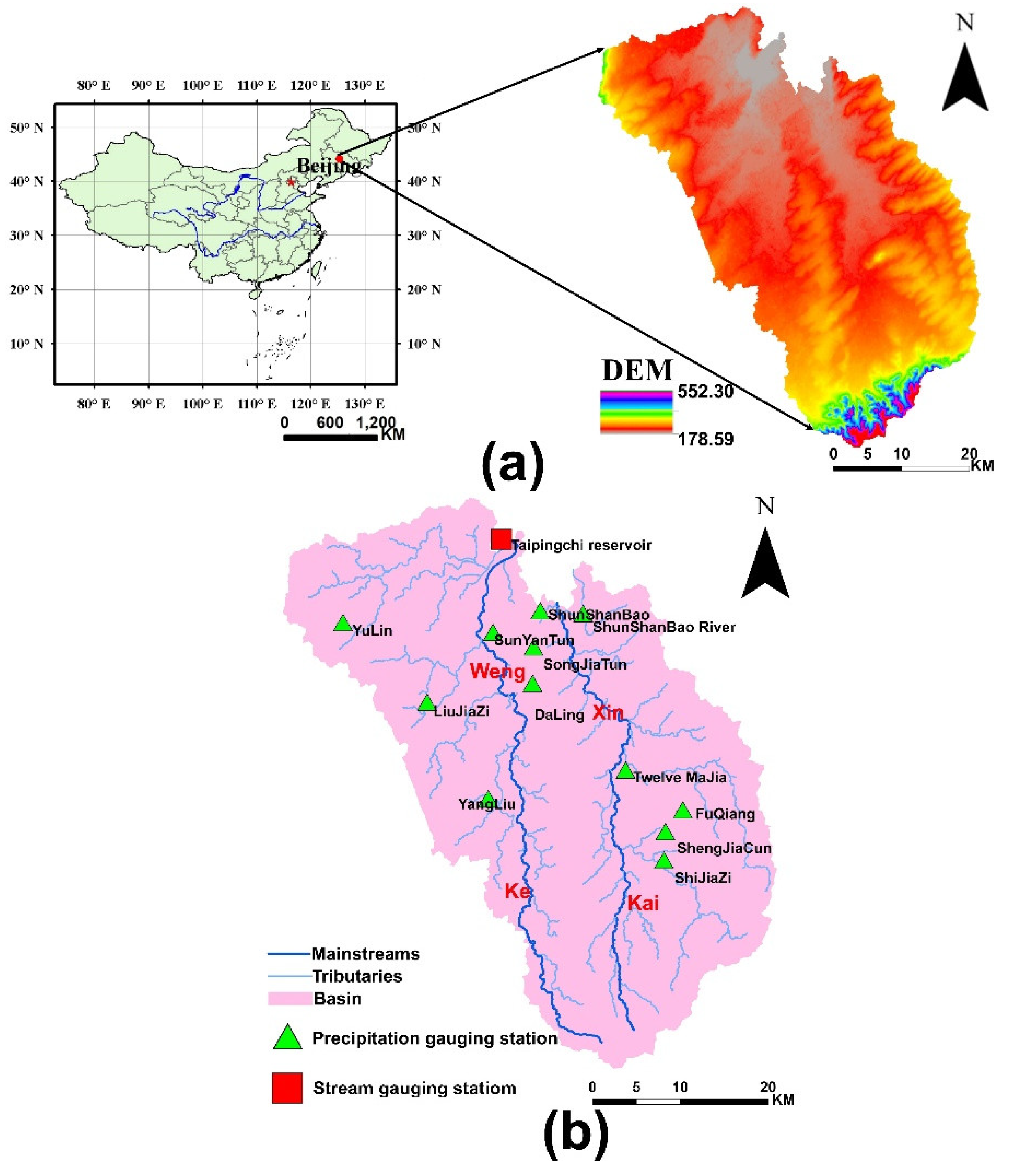
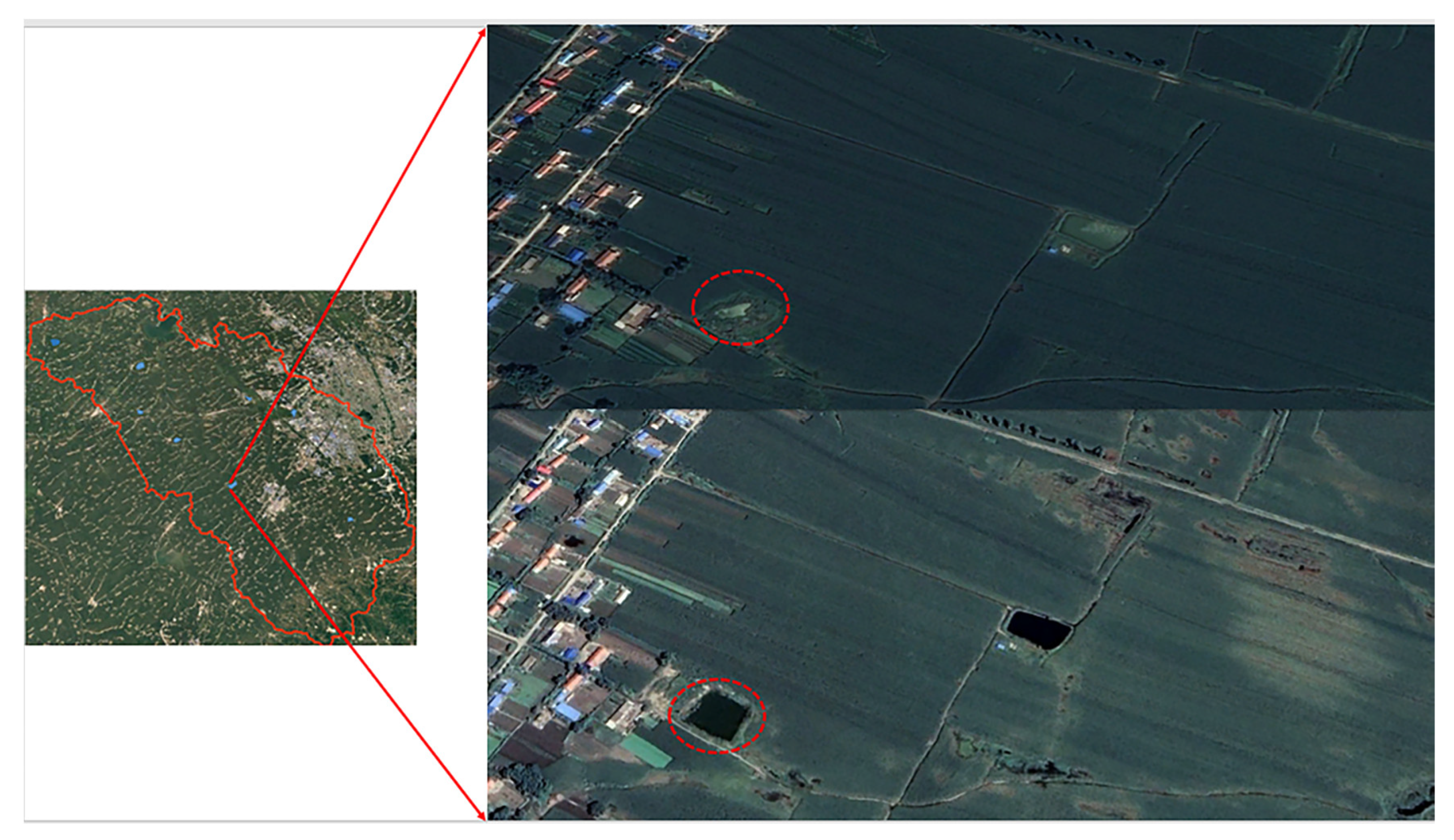
2.3. Study Area and Data Set

In the piecewise-function-described L-XAJ model, the more diverse the land-use types of the basin are, the more segments the curve is divided into and the more accurate it is to describe the water storage capacity with a continuous curve. As a result, a basin with simple land-use form and homogeneous soil is more suitable to verify the L-XAJ model. Therefore, Taipingchi basin was chosen as the study area.
Taipingchi basin, located in northeast China (Figure 8a), has an area of 1706 km2. Two tributaries, the Wengke River and the Xinkai River, flow into the mainstream of Taipingchi (Figure 8b). The elevation of the whole basin from the northwest to the southeast gradually increases, from 178 m to 552 m, with gentle fluctuations (Figure 8a). The main landform type in the basin is valley plains. Taipingchi basin is a typical human activity-dominated basin. Almost all of the basin has been built into towns or reclaimed as farmland. Urban and agricultural land account for above 95% of the total area of the basin (urban about 10% and agricultural land about 85%). According to the L-XAJ model, we guess the continuous water storage capacity curve would not be accurate enough to describe the real situation accurately as possible and the XAJ model would not perform well in this basin.
The basin is dominated by a typical semi-arid and semi-humid climate. The average annual temperature in the basin is about 4.9 °C. The annual average precipitation is 515.7 mm. Seventy percent of rainfall is in the summer from July to September. In the main flood season, July and August are prone to short-term heavy rainfall, which can easily lead to heavy flood disasters. The inter-annual variability of precipitation is large and the distribution is extremely uneven during the year. The annual average evaporation in the basin is about 947 mm.
The hydrological data mainly include the 21 flood events of 12 hydrological observation stations in the Taipingchi basin from 2009 to 2012 and 1 runoff observation station (Figure 8b), including average rainfall and runoff data (Δt = 6 h).
Based on 30 m Landsat TM image data (the data set is provided by Geospatial Data Cloud site, Computer Network Information Center, Chinese Academy of Sciences (http://www.gscloud.cn, (accessed on 24 February 2022))) and in consideration of the impact of land characteristics on runoff, the supervised classification method (by the maximum likelihood classification in ArcGIS) was adopted to classify the land-use types into five categories: forest, crops, grassland, surface water bodies, and urban (Figure 9). See Table 1 for statistical information.

2.4. Modeling Set

In this study, 21 flood events from 2009 to 2012 that took place in the Taipingchi basin were used for model calibration and verification at a 6-h time step. Fifteen flood events were chosen to calibrate the model parameters and six events to verify the model. Calibration and optimization of XAJ model parameters were based on the parameter estimation algorithm (PEST) with MATLAB environment [69]. Thirteen parameters related to evapotranspiration, runoff generation, runoff source partition and runoff routing (Table 2) were calibrated. There are three main factors to consider in the calibration process: the lower and upper boundaries [23], the objective function and termination condition. The objective function can be updated as below:
OF = i = 1 n ( Q s     Q o ) 2
where OF is objective function, i is the time order, n is the time step, Q s is the simulated discharge and Q o is the observed discharge.
L-XAJ model and XAJ model are slightly different in the parameter calibration process of runoff yield module: the WUM, WLM, WDM and B are the parameters by the XAJ, however, these parameters are replaced by the area ratios of specific land-use type (Ra1 and Ra2) and their corresponding water storage capacity values (W1 and W2) in L-XAJ. The remaining parameters are the same in both XAJ and L-XAJ. See Table 2 for parameter results.

2.5. Statistical Criteria

According to the accuracy standard for hydrological forecasting in China, the results were evaluated by three statistical criteria including the Nash–Sutcliffe efficiency coefficient (NSE), the flood volume error (FVE) and the flood peak error (FPE). The detailed equations are expressed as follows:
NSE = 1       ( Q o     Q s ) 2   ( Q o     Q o ¯ ) 2
FVE =   Q s       Q o   Q o × 100 %
FPE = MAX ( Q s )     MAX ( Q o ) MAX ( Q o ) × 100 %
where Q o is the observed discharge (m3/s), Q s is the simulated discharge (m3/s), Q o ¯ is the mean value of the observed discharge (m3/s), MAX ( Q s ) is the simulated peak discharge and MAX ( Q o ) is the observed peak discharge.
According to the accuracy standard, when NSE exceeds 0.9, it is considered to meet standard A and when 0.7 ≤ NSE ≤ 0.9, it meets standard B.

3. Results and Discussions

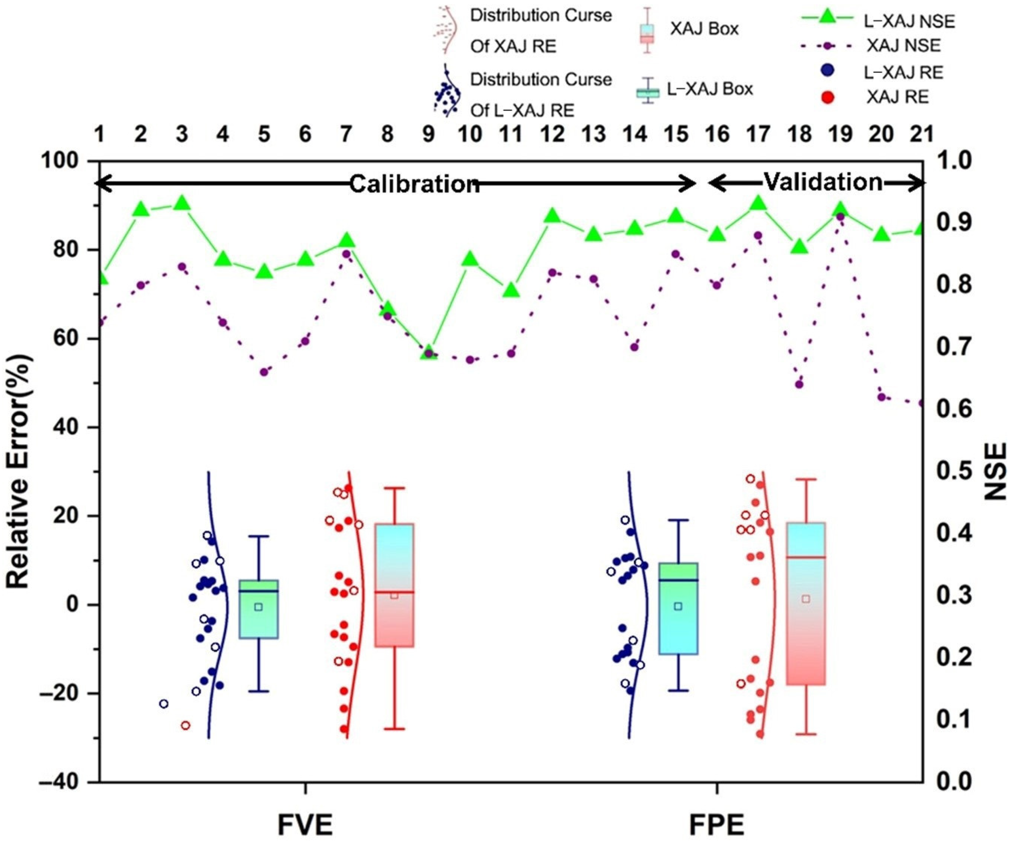
3.1. Simulated Results and Global Analysis

Both the L-XAJ model and XAJ model were applied in the Taipingchi basin. From 2009 to 2012, a total of 21 flood events occurred in the Taipingchi basin and they were all simulated by these two models. The performances of the two models were tested by the statistical indicators (NSE, FVE, FPE) mentioned in Section 2.5, and showed in Table 3.
As shown in Table 3, the NSE of the L-XAJ model ranged from 0.69 to 0.93, with the average being 0.86. Meanwhile, the NSE of the XAJ model ranged from 0.61 to 0.91, with the average being 0.75. For the FVE and FPE, all 21 flood events of the L-XAJ model were within 20% and the qualified rate was 100%. However, there were only 12 flood events within 20% of the FPE in the XAJ model and the qualified rate only was 57.14%. The L-XAJ model reduced the average FPE from 19.16% to 11.10% and the FVE from 14.03% to 8.87%. Overall, only 10 flood events were simulated accurately in the XAJ model, while all flood events were accurately simulated by the L-XAJ model; the simulation results of the L-XAJ model were better than the XAJ model under all the three statistical criteria. This showed that the L-XAJ model was successfully used in the Taipingchi basin.
The distributions of the FVE, FPE and NSE statistics for all simulations (both calibration and validation events) were showed in Figure 10. The NSE of the L-XAJ model was higher than the XAJ model (except 20101010) and the FPE and FVE distribution of the L-XAJ model was lower than the XAJ model. This showed that the performance of the L-XAJ model in the Taipingchi basin was comprehensively better than that of XAJ model.
Several rainfall–runoff processes were shown in Figure 11. The discharge process of the XAJ model and the L-XAJ model were basically similar and there was only a certain difference in the flood volume, indicating that the two models had the same runoff sources partition and runoff concentration and differ only in the runoff generation. The discharge processes of the two models were similar with the observed discharge (OBQ), indicating that the two models can reflect the runoff process.
Focusing on the calibration period, as the parameters of the XAJ model were calibrated by these 15 floods, it should be expected to perform well in this period. However, none of the NSE achieved standard A and three flood events of FVE and four flood events of FPE exceeded 20%, which indicates that the XAJ model is not accurate enough to reproduce the rainfall–runoff process. This is in line with our prediction in Section 2.3. In contrast, the L-XAJ model performed well during the calibration period, though its parameters were calibrated by the XAJ model. The NSE of four flood events achieved standard A and all the FVE and FPE are within 20%. The results indicated that the L-XAJ model could reflect the rainfall–runoff process more accurately; or more precisely, the land-use-based water storage capacity curve is more accurate in illustrating the runoff yield in the Taipingchi basin. Furthermore, it indicated that the land-use area ratio (L/F) is substantially associated with the yielding area (f/F) of the XAJ model, which validates the hypothesis of a corresponding relationship between the different land-use types and the yield area.
As for the validation period, the NSE of the L-XAJ model had two flood events for standard A and four for standard B in all of the six floods, while all the FVE and FPE were within 20%. The validation results performed well.
Generally, the performance of the XAJ model in the Taipingchi basin is mediocre, which indicated that the XAJ model would not perform well in a simple land-use basin. On the other hand, the L-XAJ model outperformed in 17 of 21 floods, not only in the validation period, but also in the calibration period. This indicated that the L-XAJ model is more suitable for simulating the hydrological process of the Taipingchi basin than the XAJ model or that the land-use-based water storage capacity curve can describe the runoff yield more accurately than the original water storage capacity curve of the XAJ model.

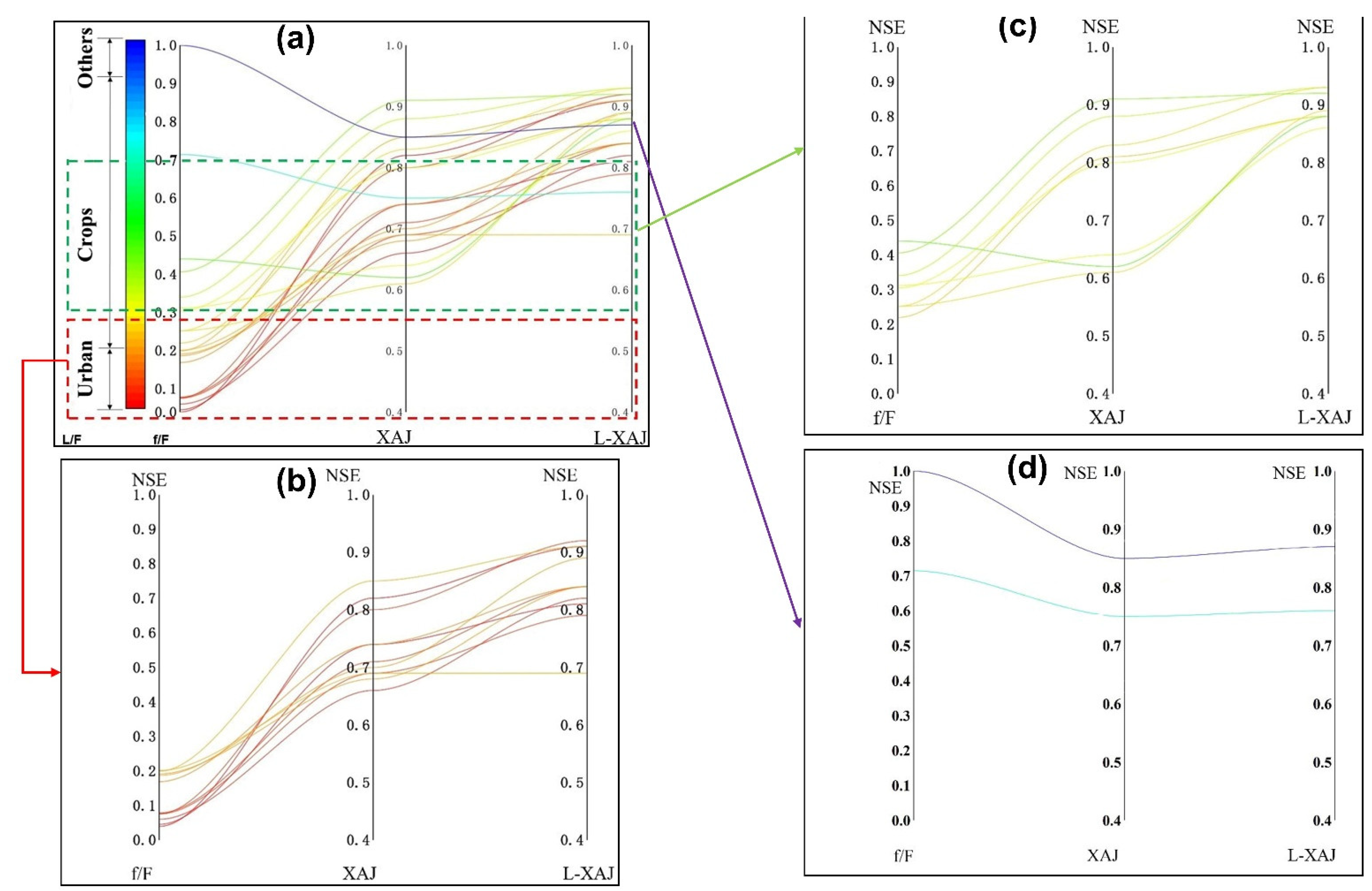
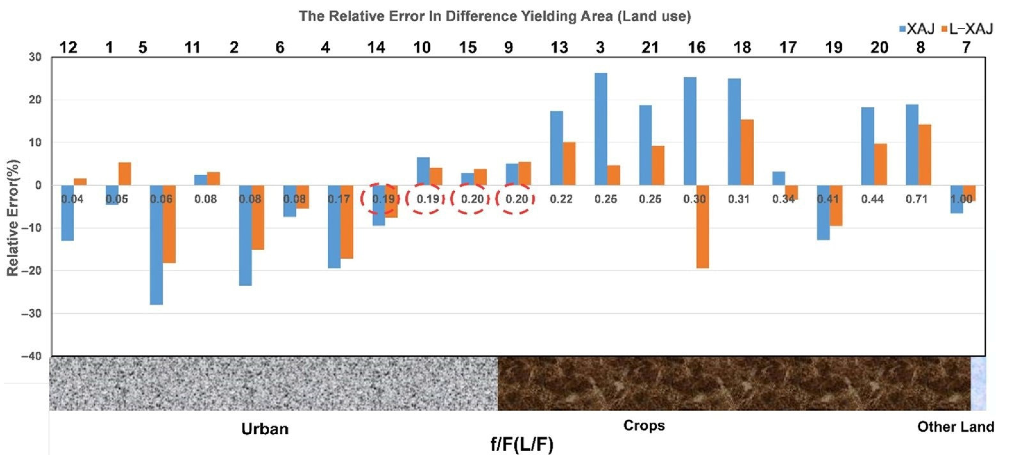
3.2. Simulation Results in Different Yielding Area

During severe rainfall events or high-intensity rainfalls, the runoff yield is not synchronized everywhere in the basin [70]. Generally, an impervious surface usually yields earlier than the other areas; farmland with low vegetation usually has less interception than forests with tall vegetation, so it yields earlier than the forest area. Under the same underlying surface type, the higher the soil moisture is, the earlier the flow is produced. That is to say, in different flood events, the actual yielding area and yielding process are different.
On the other hand, a rainfall–runoff model ignoring the underlying surface would perform differently from a model based on land-use form. This difference would be changed by the yielding area and can be shown in Figure 12. As the urban area takes up about 20% of the basin area and crops take up above 70%, the total yielding area (Figure 12a) can be separated easily from each other, such as (0, 0.2) (Figure 12b), [0.2, 0.7] (Figure 12c) and (0.7, 1] (Figure 12d). The larger the yielding area, the smaller difference of the NSE between the XAJ model and L-XAJ model (Figure 12a): when the yielding area was small (Figure 12b), the basin was relatively dry and the impact of 20% of the urban area on the runoff generation was reflected in the L-XAJ model, which can make up for the artificially intercepted rainfall, so the NSE is higher; when the yielding area increases (Figure 12c), the basin was relatively humid and the level of 70% crops was reflected. At this stage, although the NSE of L-XAJ has been improved relative to XAJ, the improvement effect is not as obvious as the previous stage (dry stage). This is because the urban and crops worked together on the runoff yield and the difference in the runoff calculation between XAJ and L-XAJ is not as large as that in the dry stage (Figure 2a and Figure 6b); when the basin was in a near-saturated state (Figure 12d), there was almost no difference between the two models and both are simulated well. These were expected due to the mechanism of land use on runoff generation [71]. These results explained the effect of different land uses on rainfall redistribution when the basin was in different stages. Hence, correspondence between the yield area (in XAJ) and land-use type (in L-XAJ) is characterized.
Figure 13 showed the FVE under different yielding areas. Under the control of the urban area, the FVE of the XAJ model was very large and the flood volume was always smaller than observed, while the L-XAJ model not. It was closely related to the influence of the urban area on the runoff yield [72]. While under the control of the crops, the flood volume was always larger than observed, which was because crops had an impact on the runoff yield [73]. The water storage capacity of crops in the Taipingchi basin was relatively large, so the runoff yield in this part was low, but the XAJ model did not consider it.
In conclusion, the land-use form influences the runoff process. It could be found that the area of different land types and its storage capacity value correspond to the yielding area of XAJ model. Hence, we verified that f/F corresponds to L/F and that the research objectives that were discussed in the introduction of this paper were met.

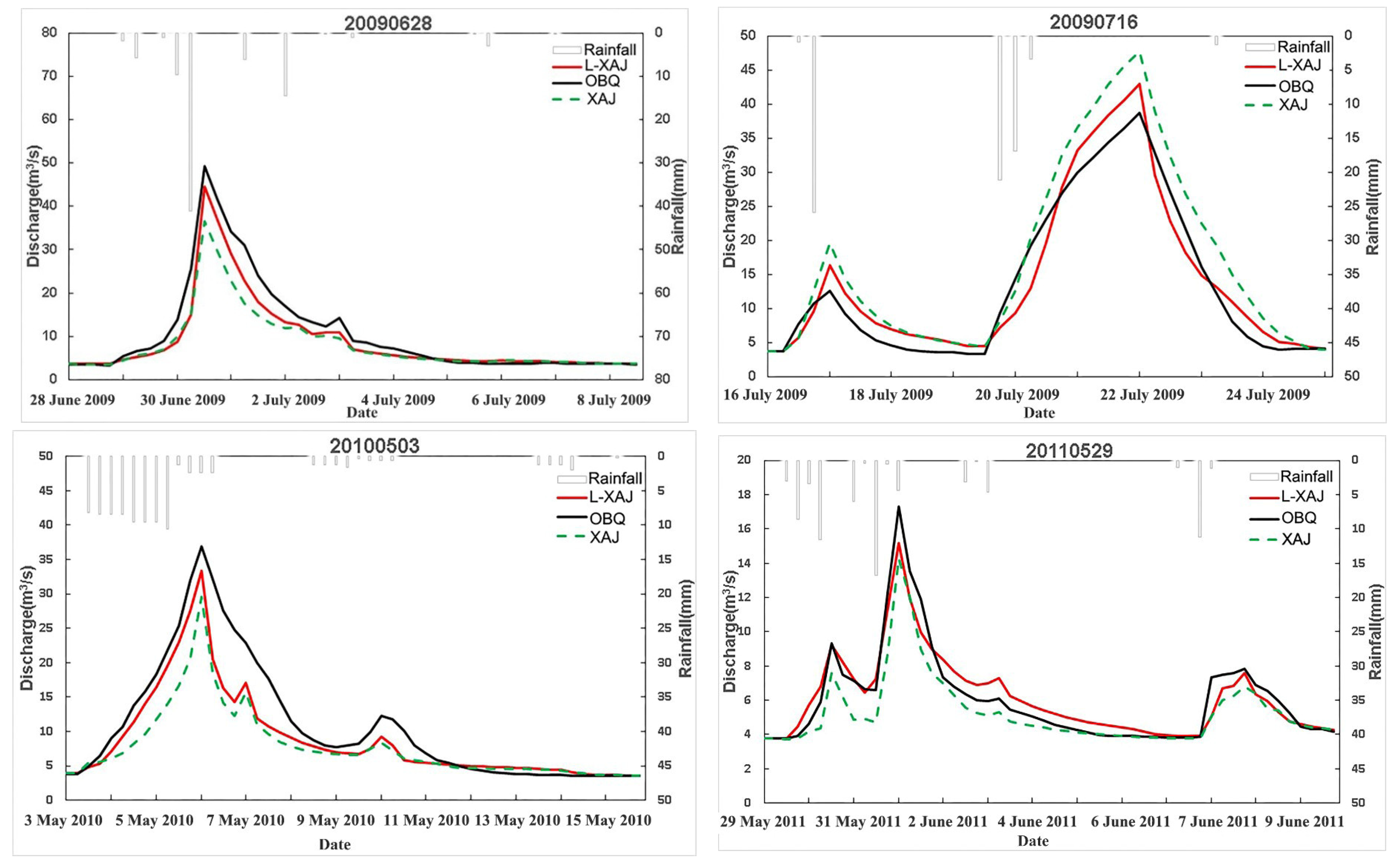
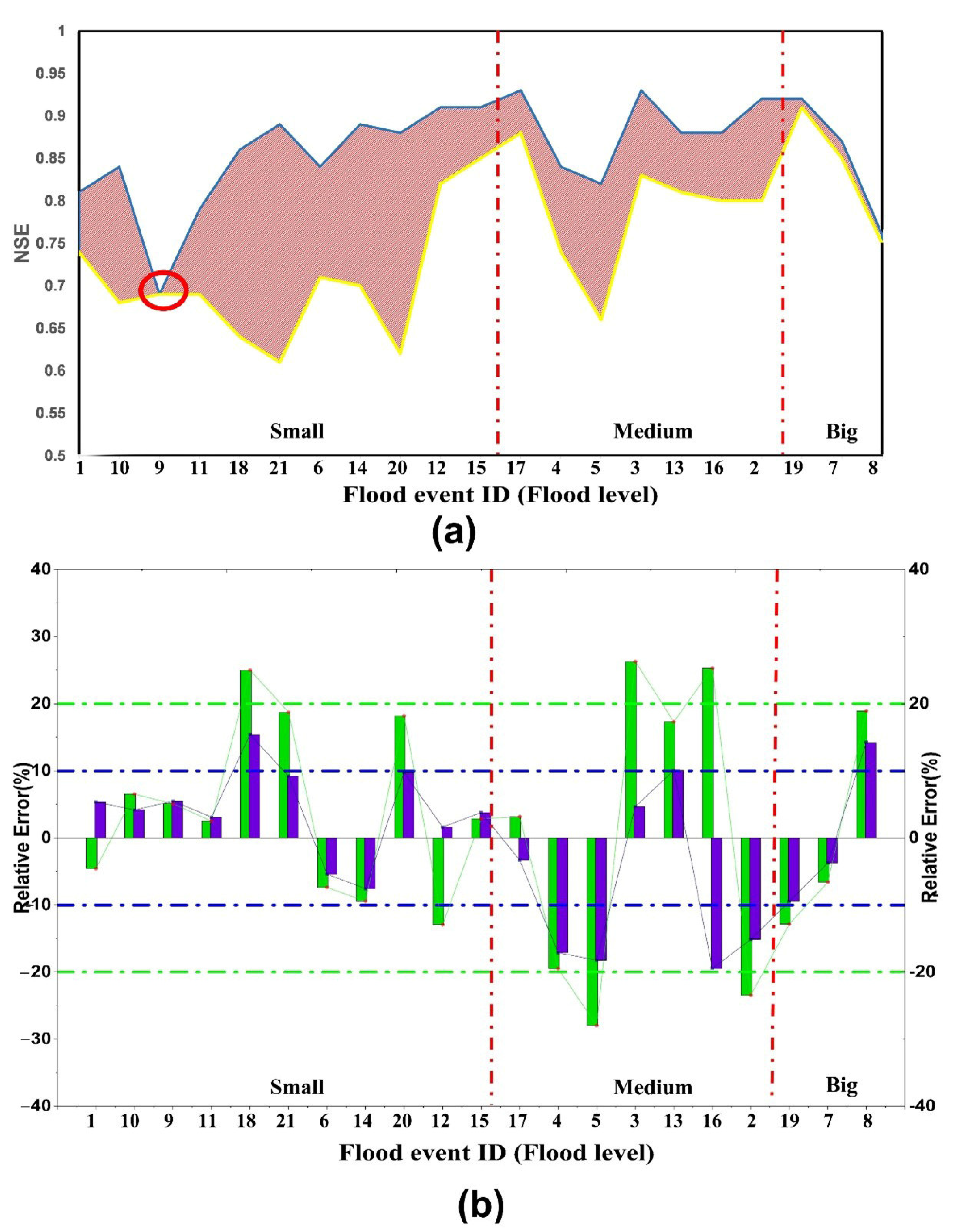
3.3. Simulation Results in Different Flood Types

In order to study the sensitivity of the XAJ model and L-XAJ model to the flood magnitude, 21 flood events were divided into three levels: large, medium and small, according to the peak discharge. There were three large flood events, seven medium flood events and eleven small flood events. The NSE and the FVE in different flood levels were shown in Figure 14.
It could be seen from Figure 14a that the NSE of the L-XAJ model was greatly improved compared with the XAJ model in small and medium floods, especially for small floods. The major reason for this was that the runoff of small floods is more easily affected by land use [71,74]. However, the third flood (circled in red in Figure 14a) had not been improved. After analysis, this might be due to the yielding area which was around 0.2 and the difference between the L-XAJ model and XAJ model was not significant.
The FVE of the different flood levels were shown in Figure 14b: for small floods, the FVE was smaller, but compared to the XAJ model, the L-XAJ model had higher accuracy; for medium floods, the FVE of the XAJ model was relatively large. This was because most of the seven medium floods were at the beginning of each year or after the flood season. At this time, for crop growth, many ponds had been artificially established in the basin to store rainfall [75] (Figure 15), which had a significant impact on the runoff yield, however, the runoff yield calculated by L-XAJ is more than that of XAJ at this stage (Figure 2a and Figure 6b), so the store rainfall can be partially offset in L-XAJ. How to consider the rainfall interception in L-XAJ is the main direction of our in-depth research. For big floods, the larger accuracy indicated a better performance of both models, which is in agreement with the relevant literature [71].
To further analyze the performance of the L-XAJ model compared to XAJ, the improved accuracy of the L-XAJ model relative to the XAJ model was analyzed and the improved results were shown in Figure 16. For the NSE, compared with the XAJ model, the L-XAJ model had a significant improvement of small and medium floods, but almost no improvement for large floods. For the FPE and FVE, in small floods, the FVE increased by 16.57% on average and the FPE by 44.76%; in medium floods, the FVE increased by 38.25% on average and the FPE by 43.42. In large floods, the FVE increased by 31.42% on average and the FPE by 2.66%. Therefore, it was further proved that the L-XAJ model can significantly improve the performance of flood simulation.
Based on the results in Section 3.2, this change can be easily explained: the runoff yield usually occurs in part of the basin in small floods and medium floods, while the runoff yield of big floods generally occurs in the entire basin.

4. Conclusions

Effective basin water resource management is of significant importance for the basin’s sustainable development. The main objective of this research is to study the relationship between the yielding area (f/F) and the area of different land uses (L/F) for better basin flood resource management. The L-XAJ model was constructed by integrating the land-use information into the runoff generation of the XAJ model and the model is shown to improve the performance of the runoff in a typical cultivated–urban binary land-use-type basin: the Taipingchi basin. The major findings of this paper were summarized as follows:
(1) The distribution of the runoff yield can be divided by the land-use form, which is, the areas with the same land-use form are similar in runoff yield, while areas of different land uses are significantly different. In the XAJ model, particularly, that is to say, the yielding area of the XAJ model, (f/F) is determined by the area ratio of different land-use types (L/F) (Section 3.2).
(2) The L-XAJ model can be well used in a rainfall–runoff simulation (Table 3 and Figure 10). It performed better than the XAJ model in a simple land-use-form basin (mean NSE: 0.86 > 0.75, FVE: 8.87% < 14.03%, FPE: 11.10% < 19.06%).
(3) The L-XAJ model can well improve the simulation accuracy of small and medium floods compared to large floods (Figure 16).
Although our preliminary test demonstrated the relationship between the runoff yield and land use, we still know little about the calculation of the runoff yield for specific areas. Ongoing research could focus on analyzing the effect of vegetation type, soil type, topography and other remotely-sensed data on the runoff yield. How to establish an index that integrates various factors to further enhance the physical meaning of the runoff generation in the XAJ model to obtain better results is worthy of further study.

5. Patents

The patent “A method and system for determining runoff yield of artificial watershed” (patent number: CN 202011611825.9) resulted from the work reported in this manuscript.

Author Contributions

Conceptualization, C.X.; Data curation, C.X.; Formal analysis, C.X.; Investigation, C.X. and H.F.; Methodology, C.X.; Project administration, H.F.; Resources, C.X. and Y.W.; Software, C.X. and J.Y.; Supervision, H.F.; Validation, C.X. and L.W.; Visualization, C.X. and Y.W.; Writing—original draft, C.X. and H.F.; Writing review and editing, J.Y., L.W. and Y.W. All authors have read and agreed to the published version of the manuscript.

Funding

This research was funded by Major Science and Technology Program for Water Pollution Control and Treatment, grant number No. 2014ZX07203-008.

Institutional Review Board Statement

Not applicable.

Informed Consent Statement

Not applicable.

Data Availability Statement

Some or all data, models, or codes that support the findings of this study are available from the corresponding author upon reasonable request.

Acknowledgments

The authors would like to acknowledge Xiaoliu Yang of Peking University, China, for his theoretical support and guidance. This research was funded by the Major Science and Technology Program for Water Pollution Control and Treatment (Grant No. 2014ZX07203-008). The authors would like to thank the Jilin Provincial Water Resources Department for providing the hydrological data for this article.

Conflicts of Interest

The authors declare no conflict of interest.

References

  1. Huang, F.; Zhang, Y.D.; Zhang, D.R.; Chen, X. Environmental Groundwater Depth for Groundwater-Dependent Terrestrial Ecosystems in Arid/Semiarid Regions: A Review. Int. J. Environ. Res. Public Health 2019, 16, 763. [Google Scholar] [CrossRef] [PubMed]
  2. Li, P.Y.; Wang, D.; Li, W.Q.; Liu, L.N. Sustainable water resources development and management in large river basins: An introduction. Environ. Earth Sci. 2022, 81, 179. [Google Scholar] [CrossRef] [PubMed]
  3. Meijer, K.S.; Schasfoort, F.; Bennema, M. Quantitative Modeling of Human Responses to Changes in Water Resources Availability: A Review of Methods and Theories. Sustainability 2021, 13, 8675. [Google Scholar] [CrossRef]
  4. Li, J.; Liu, C.M.; Wang, Z.G.; Liang, K. Two universal runoff yield models: SCS vs. LCM. J. Geogr. Sci. 2015, 25, 311–318. [Google Scholar] [CrossRef]
  5. Zhang, J.P.; Zhang, H.; Xiao, H.L.; Fang, H.Y.; Han, Y.P.; Yu, L. Effects of rainfall and runoff-yield conditions on runoff. Ain Shams Eng. J. 2021, 12, 2111–2116. [Google Scholar] [CrossRef]
  6. Gupta, S.K.; Tyagi, J.; Sharma, G.; Jethoo, A.S.; Singh, P.K. An Event-Based Sediment Yield and Runoff Modeling Using Soil Moisture Balance/Budgeting (SMB) Method. Water Resour. Manag. 2019, 33, 3721–3741. [Google Scholar] [CrossRef]
  7. Dunne, T.; Black, R.D. Partial Area Contributions to Storm Runoff in a Small New-England Watershed. Water Resour. Res. 1970, 6, 1296–1311. [Google Scholar] [CrossRef]
  8. Horton; Robert, E. The role of infiltration in the hydrologic cycle. Trans. Am. Geophys. Union 1933, 14, 446–460. [Google Scholar] [CrossRef]
  9. Bennett, J.C.; Wang, Q.; Li, M.; Robertson, D.; Schepen, A. Reliable long-range ensemble streamflow forecasts by combining dynamical climate forecasts: A conceptual runoff model and a staged error model. Water Resour. Res. 2016, 52, 8238–8259. [Google Scholar] [CrossRef]
  10. Kan, G.; He, X.; Ding, L.; Li, J.; Liang, K.; Hong, Y. Study on applicability of conceptual hydrological models for flood forecasting in humid, semi-humid semi-arid and arid basins in China. Water 2017, 9, 719. [Google Scholar] [CrossRef] [Green Version]
  11. Zhang, L.; Yang, X. Applying a Multi-Model Ensemble Method for Long-Term Runoff Prediction under Climate Change Scenarios for the Yellow River Basin, China. Water 2018, 10, 301. [Google Scholar] [CrossRef]
  12. De Barros, C.; Minella, J.; Schlesner, A.; Ramon, R.; Copetti, A. Impact of data sources to DEM construction and application to runoff and sediment yield modelling using LISEM model. J. Earth Syst. Sci. 2021, 130, 53. [Google Scholar] [CrossRef]
  13. Nazari-Sharabian, M.; Taheriyoun, M.; Karakouzian, M. Sensitivity analysis of the DEM resolution and effective parameters of runoff yield in the SWAT model: A case study. J. Water Supply Res. Technol. 2020, 69, 39–54. [Google Scholar] [CrossRef]
  14. Zhao, R.J. The Xinanjiang Model Applied in China. J. Hydrol. 1992, 135, 371–381. [Google Scholar] [CrossRef]
  15. Tran, Q.Q.; De Niel, J.; Willems, P. Spatially Distributed Conceptual Hydrological Model Building: A Genetic top-Down Approach Starting from Lumped Models. Water Resour. Res. 2018, 54, 8064–8085. [Google Scholar] [CrossRef]
  16. Zhang, R.; Cuartas, L.A.; Carvalho, L.V.D.; Leal, K.R.D.; Mendiondo, E.M.; Abe, N.; Birkinshaw, S.; Mohor, G.S.; Seluchi, M.E.; Nobre, C.A. Season-based rainfall-runoff modelling using the probability-distributed model (PDM) for large basins in southeastern Brazil. Hydrol. Process. 2018, 32, 2217–2230. [Google Scholar] [CrossRef]
  17. Gong, J.F.; Yao, C.; Li, Z.J.; Chen, Y.F.; Huang, Y.C.; Tong, B.X. Improving the flood forecasting capability of the Xinanjiang model for small- and medium-sized ungauged catchments in South China. Nat. Hazards 2021, 106, 2077–2109. [Google Scholar] [CrossRef]
  18. Wang, J.; Bao, W.M.; Gao, Q.Y.; Si, W.; Sun, Y.Q. Coupling Xinanjiang model and wavelet-based random forests method for improved daily streamflow simulation. J. Hydroinform. 2021, 23, 589–604. [Google Scholar] [CrossRef]
  19. Xu, C.W.; Han, Z.Y.; Fu, H. Remote Sensing and Hydrologic-Hydrodynamic Modeling Integrated Approach for Rainfall-Runoff Simulation in Farm Dam Dominated Basin. Front. Environ. Sci. 2022, 9, 672. [Google Scholar] [CrossRef]
  20. Zuo, D.P.; Xu, Z.X.; Yao, W.Y.; Jin, S.Y.; Xiao, P.Q.; Ran, D.C. Assessing the effects of changes in land use and climate on runoff and sediment yields from a watershed in the Loess Plateau of China. Sci. Total Environ. 2016, 544, 238–250. [Google Scholar] [CrossRef]
  21. Paule-Mercado, M.A.; Lee, B.Y.; Memon, S.A.; Umer, S.R.; Salim, I.; Lee, C.H. Influence of land development on stormwater runoff from a mixed land use and land cover catchment. Sci. Total Environ. 2017, 599, 2142–2155. [Google Scholar] [CrossRef]
  22. Meng, C.Q.; Zhou, J.Z.; Zhong, D.Y.; Wang, C.; Guo, J. An Improved Grid-Xinanjiang Model and Its Application in the Jinshajiang Basin, China. Water 2018, 10, 1265. [Google Scholar] [CrossRef]
  23. Yao, C.; Zhang, K.; Yu, Z.B.; Li, Z.J.; Li, Q.L. Improving the flood prediction capability of the Xinanjiang model in ungauged nested catchments by coupling it with the geomorphologic instantaneous unit hydrograph. J. Hydrol. 2014, 517, 1035–1048. [Google Scholar] [CrossRef]
  24. Xu, Y.Y.; Cheng, X.; Gun, Z. What Drove Regional Changes in the Number and Surface Area of Lakes across the Yangtze River Basin during 2000–2019: Human or Climatic Factors? Water Resour. Res. 2022, 58, e2021WR030616. [Google Scholar] [CrossRef]
  25. Yan, X.L.; Bao, Z.X.; Zhang, J.Y.; Wang, G.Q.; He, R.M.; Liu, C.S. Quantifying contributions of climate change and local human activities to runoff decline in the upper reaches of the Luanhe River basin. J. Hydro-Environ. Res. 2020, 28, 67–74. [Google Scholar] [CrossRef]
  26. Wang, G.; Yinglan, A.; Xu, Z.; Zhang, S. The influence of land use patterns on water quality at multiple spatial scales in a river system. Hydrol. Process. 2015, 28, 5259–5272. [Google Scholar] [CrossRef]
  27. Wagener, T. Can we model the hydrological impacts of environmental change? Hydrol. Process. 2007, 21, 3233–3236. [Google Scholar] [CrossRef]
  28. Zhu, W.B.; Jia, S.F.; Lall, U.; Cao, Q.; Mahmood, R. Relative contribution of climate variability and human activities on the water loss of the Chari/Logone River discharge into Lake Chad: A conceptual and statistical approach. J. Hydrol. 2019, 569, 519–531. [Google Scholar] [CrossRef]
  29. Zheng, H.X.; Zhang, L.; Zhu, R.R.; Liu, C.M.; Sato, Y.; Fukushima, Y. Responses of streamflow to climate and land surface change in the headwaters of the Yellow River Basin. Water Resour. Res. 2009, 45. [Google Scholar] [CrossRef]
  30. Gao, H.K.; Cai, H.Y.; Duan, Z. Understanding the impacts of catchment characteristics on the shape of the storage capacity curve and its influence on flood flows. Hydrol. Res. 2018, 49, 90–106. [Google Scholar] [CrossRef]
  31. Jayawardena, A.; Zhou, M. A modified spatial soil moisture storage capacity distribution curve for the Xinanjiang model. J. Hydrol. 2000, 227, 93–113. [Google Scholar] [CrossRef]
  32. Shi, P.F.; Yang, T.; Xu, C.Y.; Yong, B.; Huang, C.S.; Li, Z.Y.; Qin, Y.W.; Wang, X.Y.; Zhou, X.D.; Li, S. Rainfall-Runoff Processes and Modelling in Regions Characterized by Deficiency in Soil Water Storage. Water 2019, 11, 1858. [Google Scholar] [CrossRef]
  33. Chang, B.X.; Wherley, B.; Aitkenhead-Peterson, J.A.; McInnes, K.J. Effects of urban residential landscape composition on surface runoff generation. Sci. Total Environ. 2021, 783, 146977. [Google Scholar] [CrossRef]
  34. Feng, X.M.; Sun, G.; Fu, B.J.; Su, C.H.; Liu, Y.; Lamparski, H. Regional effects of vegetation restoration on water yield across the Loess Plateau, China. Hydrol. Earth Syst. Sci. 2012, 16, 2617–2628. [Google Scholar] [CrossRef]
  35. Xu, Y.Y.; Li, J.; Wang, J.D.; Chen, J.L.; Liu, Y.B.; Ni, S.N.; Zhang, Z.Z.; Ke, C.Q. Assessing water storage changes of Lake Poyang from multi-mission satellite data and hydrological models. J. Hydrol. 2020, 590, 125229. [Google Scholar] [CrossRef]
  36. Sajikumar, N.; Remya, R.S. Impact of land cover and land use change on runoff characteristics. J. Environ. Manag. 2015, 161, 460–468. [Google Scholar] [CrossRef]
  37. Astuti, I.S.; Sahoo, K.; Milewski, A.; Mishra, D.R. Impact of land use land cover (LULC) change on surface runoff in an increasingly urbanized tropical watershed. Water Resour. Manag. 2019, 33, 4087–4103. [Google Scholar] [CrossRef]
  38. Zhou, M.; Qu, S.; Chen, X.; Shi, P.; Xu, S.; Chen, H.; Zhou, H.; Gou, J. Impact Assessments of Rainfall–Runoff Characteristics Response Based on Land Use Change via Hydrological Simulation. Water 2019, 11, 866. [Google Scholar] [CrossRef]
  39. Rogger, M.; Agnoletti, M.; Alaoui, A.; Bathurst, J.C.; Bodner, G.; Borga, M.; Chaplot, V.; Gallart, F.; Glatzel, G.; Hall, J. Land-use change impacts on floods at the catchment scale: Challenges and opportunities for future research. Water Resour. Res. 2017, 53, 5209–5219. [Google Scholar] [CrossRef]
  40. Farsi, N.; Mahjouri, N. Evaluating the contribution of the climate change and human activities to runoff change under uncertainty. J. Hydrol. 2019, 574, 872–891. [Google Scholar] [CrossRef]
  41. Yang, L.; Feng, Q.; Yin, Z.; Wen, X.; Si, J.; Li, C.; Deo, R.C. Identifying separate impacts of climate and land use/cover change on hydrological processes in upper stream of Heihe River, Northwest China. Hydrol. Process. 2017, 31, 1100–1112. [Google Scholar] [CrossRef]
  42. Walega, A.; Salata, T. Influence of land cover data sources on estimation of direct runoff according to SCS-CN and modified SME methods. Catena 2019, 172, 232–242. [Google Scholar] [CrossRef]
  43. Yin, J.; He, F.; Xiong, Y.J.; Qiu, G.Y. Effects of land use/land cover and climate changes on surface runoff in a semi-humid and semi-arid transition zone in northwest China. Hydrol. Earth Syst. Sci. 2017, 21, 183–196. [Google Scholar] [CrossRef]
  44. Chen, Y.; Xu, C.Y.; Chen, X.W.; Xu, Y.P.; Yin, Y.X.; Gao, L.; Liu, M.B. Uncertainty in simulation of land-use change impacts on catchment runoff with multi-timescales based on the comparison of the HSPF and SWAT models. J. Hydrol. 2019, 573, 486–500. [Google Scholar] [CrossRef]
  45. Guo, M.; Zhang, T.; Li, Z.; Xu, G. Investigation of runoff and sediment yields under different crop and tillage conditions by field artificial rainfall experiments. Water 2019, 11, 1019. [Google Scholar] [CrossRef]
  46. Li, T.; Dong, J.; Yuan, W. Effects of Precipitation and Vegetation Cover on Annual Runoff and Sediment Yield in Northeast China: A Preliminary Analysis. Water Resour. 2020, 47, 491–505. [Google Scholar] [CrossRef]
  47. Liu, J.; Gao, G.; Wang, S.; Jiao, L.; Wu, X.; Fu, B. The effects of vegetation on runoff and soil loss: Multidimensional structure analysis and scale characteristics. J. Geogr. Sci. 2018, 28, 59–78. [Google Scholar] [CrossRef]
  48. Nourani, V.; Fard, A.F.; Gupta, H.V.; Goodrich, D.C.; Niazi, F. Hydrological model parameterization using NDVI values to account for the effects of land cover change on the rainfall–runoff response. Hydrol. Res. 2017, 48, 1455–1473. [Google Scholar] [CrossRef]
  49. Oudin, L.; Salavati, B.; Furusho-Percot, C.; Ribstein, P.; Saadi, M. Hydrological impacts of urbanization at the catchment scale. J. Hydrol. 2018, 559, 774–786. [Google Scholar] [CrossRef]
  50. Kim, Y.D.; Kim, J.M.; Kang, B. Projection of runoff and sediment yield under coordinated climate change and urbanization scenarios in Doam dam watershed, Korea. J. Water Clim. Chang. 2017, 8, 235–253. [Google Scholar] [CrossRef]
  51. Schilling, K.E.; Chan, K.-S.; Liu, H.; Zhang, Y.-K. Quantifying the effect of land use land cover change on increasing discharge in the Upper Mississippi River. J. Hydrol. 2010, 387, 343–345. [Google Scholar] [CrossRef]
  52. Levavasseur, F.; Bailly, J.S.; Lagacherie, P.; Colin, F.; Rabotin, M. Simulating the effects of spatial configurations of agricultural ditch drainage networks on surface runoff from agricultural catchments. Hydrol. Process. 2012, 26, 3393–3404. [Google Scholar] [CrossRef]
  53. da Silva, R.M.; Santos, C.A.G.; dos Santos, J.Y.G. Evaluation and modeling of runoff and sediment yield for different land covers under simulated rain in a semiarid region of Brazil. Int. J. Sediment. Res. 2018, 33, 117–125. [Google Scholar] [CrossRef]
  54. Zhang, S.; Li, Z.; Lin, X.; Zhang, C. Assessment of Climate Change and Associated Vegetation Cover Change on Watershed-Scale Runoff and Sediment Yield. Water 2019, 11, 1373. [Google Scholar] [CrossRef]
  55. Sinha, R.K.; Eldho, T. Effects of historical and projected land use/cover change on runoff and sediment yield in the Netravati river basin, Western Ghats, India. Environ. Earth Sci. 2018, 77, 111. [Google Scholar] [CrossRef]
  56. Narimani, R.; Erfanian, M.; Nazarnejad, H.; Mahmodzadeh, A. Evaluating the impact of management scenarios and land use changes on annual surface runoff and sediment yield using the GeoWEPP: A case study from the Lighvanchai watershed, Iran. Environ. Earth Sci. 2017, 76, 353. [Google Scholar] [CrossRef]
  57. Hu, S.; Fan, Y.; Zhang, T. Assessing the effect of land use change on surface runoff in a rapidly urbanized city: A case study of the central area of Beijing. Land 2020, 9, 17. [Google Scholar] [CrossRef]
  58. Li, F.; Chen, J.; Liu, Y.; Xu, P.; Sun, H.; Engel, B.A.; Wang, S. Assessment of the impacts of land use/cover change and rainfall change on surface runoff in China. Sustainability 2019, 11, 3535. [Google Scholar] [CrossRef]
  59. Erena, S.H.; Worku, H. Dynamics of land use land cover and resulting surface runoff management for environmental flood hazard mitigation: The case of Dire Daw city, Ethiopia. J. Hydrol. Reg. Stud. 2019, 22, 100598. [Google Scholar] [CrossRef]
  60. Guo, X.; Li, T.; He, B.; He, X.; Yao, Y. Effects of land disturbance on runoff and sediment yield after natural rainfall events in southwestern China. Environ. Sci. Pollut. Res. 2017, 24, 9259–9268. [Google Scholar] [CrossRef]
  61. Aghakhani, M.; Nasrabadi, T.; Vafaeinejad, A. Assessment of the effects of land use scenarios on watershed surface runoff using hydrological modelling. Appl. Ecol. Environ. Res. 2018, 16, 2369–2389. [Google Scholar] [CrossRef]
  62. Yini, H.; Jianzhi, N.; Zhongbao, X.; Wei, Z.; Tielin, Z.; Xilin, W.; Yousong, Z. Optimization of land use pattern reduces surface runoff and sediment loss in a Hilly-Gully watershed at the Loess Plateau, China. For. Syst. 2016, 25, 9. [Google Scholar] [CrossRef]
  63. Ma, K.; Huang, X.R.; Liang, C.; Zhao, H.B.; Zhou, X.Y.; Wei, X.Y. Effect of land use/cover changes on runoff in the Min River watershed. River Res. Appl. 2020, 36, 749–759. [Google Scholar] [CrossRef]
  64. Zhang, H.; Wang, B.; Liu, D.L.; Zhang, M.X.; Leslie, L.M.; Yu, Q. Using an improved SWAT model to simulate hydrological responses to land use change: A case study of a catchment in tropical Australia. J. Hydrol. 2020, 585, 124822. [Google Scholar] [CrossRef]
  65. Wang, Y.P.; Wang, S.; Wang, C.; Zhao, W.W. Runoff sensitivity increases with land use/cover change contributing to runoff decline across the middle reaches of the Yellow River basin. J. Hydrol. 2021, 600, 126536. [Google Scholar] [CrossRef]
  66. Zhang, J.; Yu, X.L. Analysis of land use change and its influence on runoff in the Puhe River Basin. Environ. Sci. Pollut. Res. 2021, 28, 40116–40125. [Google Scholar] [CrossRef]
  67. Bartlett, M.S.; Daly, E.; McDonnell, J.J.; Parolari, A.J.; Porporato, A. Stochastic rainfall-runoff model with explicit soil moisture dynamics. Proc. R. Soc. A Math. Phys. Eng. Sci. 2015, 471, 20150389. [Google Scholar] [CrossRef]
  68. Chen, X.; Chen, Y.D.; Xu, C.Y. A distributed monthly hydrological model for integrating spatial variations of basin topography and rainfall. Hydrol. Process. 2007, 21, 242–252. [Google Scholar] [CrossRef]
  69. Goegebeur, M.; Pauwels, V.R.N. Improvement of the PEST parameter estimation algorithm through Extended Kalman Filtering. J. Hydrol. 2007, 337, 436–451. [Google Scholar] [CrossRef]
  70. Beven, K.J.; Kirkby, M.J. A physically based, variable contributing area model of basin hydrology/Un modèle à base physique de zone d’appel variable de l’hydrologie du bassin versant. Hydrol. Sci. J. 1979, 24, 43–69. [Google Scholar] [CrossRef] [Green Version]
  71. Zhang, Y.; Zhao, Y.; Wang, Q.M.; Wang, J.H.; Li, H.H.; Zhai, J.Q.; Zhu, Y.N.; Li, J.Z. Impact of Land Use on Frequency of Floods in Yongding River Basin, China. Water 2016, 8, 401. [Google Scholar] [CrossRef]
  72. Zhang, L.M.; Meng, X.Y.; Wang, H.; Yang, M.X. Simulated Runoff and Sediment Yield Responses to Land-Use Change Using the SWAT Model in Northeast China. Water 2019, 11, 915. [Google Scholar] [CrossRef]
  73. Zumr, D.; Dostal, T.; Devaty, J. Identification of prevailing storm runoff generation mechanisms in an intensively cultivated catchment. J. Hydrol. Hydromech. 2015, 63, 246–254. [Google Scholar] [CrossRef]
  74. Bian, G.D.; Du, J.K.; Song, M.M.; Zhang, X.L.; Zhang, X.Q.; Li, R.J.; Wu, S.Y.; Duan, Z.; Xu, C.Y. Detection and attribution of flood responses to precipitation change and urbanization: A case study in Qinhuai River Basin, Southeast China. Hydrol. Res. 2020, 51, 351–365. [Google Scholar] [CrossRef]
  75. Yu, X.Y.; He, X.Y.; Zheng, H.F.; Guo, R.C.; Ren, Z.B.; Zhang, D.; Lin, J.X. Spatial and temporal analysis of drought risk during the crop-growing season over northeast China. Nat. Hazards 2014, 71, 275–289. [Google Scholar] [CrossRef]
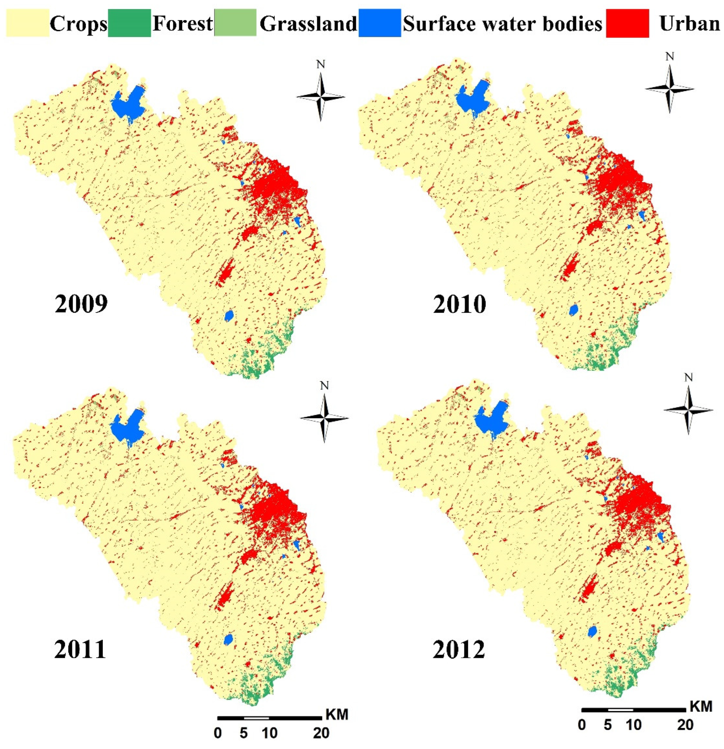
Figure 1. The framework of XAJ model. (Variables: P: precipitation; EM: potential evapotranspiration; E: actual evapotranspiration; RIM: runoff from the impervious area; RS: surface runoff; RSS: interflow runoff; RG: groundwater runoff; TRS: outflows from the reservoirs of surface run-off components; TRSS: outflows from the reservoirs of interflow run-off components; TRG: outflows from the reservoirs of groundwater run-off components; QRS: surface runoff inflow to river network; QRSS: interflow to river network; QRG: groundwater inflow to river network; s: water content in free water store reservoir; FR: ratio of runoff-producing area; Upper layer, Lower layer and Deep layer are the three soil layers for evapotranspiration; S: free water storage reservoir; UH: unit hydrograph; WM: the average water storage capacity; W m : the water storage capacity; W mm : the maximum value of W m ; EU, EL and ED are evaporation from the upper, lower and deepest layer, respectively; Q: the discharge at the outlet of the basin; Parameters: the others are parameters and will be introduced in Section 2.4).
Sustainability 14 10895 g001
Figure 2. (a) The water storage capacity curve; (b) Rainfall–runoff relationship.
Sustainability 14 10895 g002
Figure 3. Flow chart of L-XAJ model.
Sustainability 14 10895 g003
Figure 4. Picture of different land-use types (examples of different land-use types with water storage capacity: (A): grassland, (B): forest, (C): urban and (D): grassland).
Sustainability 14 10895 g004
Figure 5. (a) Schematic diagram of the area ratio of different land-use types in the basin; (b) relationship between storage capacity value and land-use types. (α1, α2, α3, α4, α5, α6 are the area ratio sums of different land-use types; w1, w2, w3, w4, w5, w6 are the average storage capacity values of different land-use types, in which w1 < w2 < w3 < w4 < w5 < w6. L/F is the area ratio of different land-use types; W m is water storage capacity; six land-use types for examples).
Sustainability 14 10895 g005
Figure 6. The construction of L-XAJ model (six land-use types for examples; (a) the lower water storage capacity values are located in smaller area and higher are in bigger area; (b) left: the basin state before rainfall for which soil moisture is W 0 ; right: the runoff process when the net rainfall is P-E, set (α3, α4] is m-th land-use type and (α4, α5] is (m + 1)th land-use type).
Sustainability 14 10895 g006
Figure 7. Rainfall–runoff relationship in L-XAJ model.
Sustainability 14 10895 g007
Figure 8. Study area information ((a): geographical location and DEM; (b) mainstream, branch and hydrological stations network).
Sustainability 14 10895 g008
Figure 9. Land-use map in the Taipingchi basin.
Sustainability 14 10895 g009
Figure 10. Comparison of the simulation results with XAJ model and L-XAJ model (the number is the order of the flood event, open circles are calibration events and filled circles are validation events).
Sustainability 14 10895 g010
Figure 11. Simulated and observed hydrographs.
Sustainability 14 10895 g011
Figure 12. The NSE in partial yielding area ((a): all yield area; (b): 0 < yield area < 0.2; (c) 0.2 ≤ yield area < 0.7; (d): yield area ≥ 0.7).
Sustainability 14 10895 g012
Figure 13. The relative error in different yielding area (different land-use types dominated, the number at the top are flood event ID).
Sustainability 14 10895 g013
Figure 14. Comparison of NSE and FVE under different flood levels ((a): NSE; (b) FVE; the green dotted line is the 20% error line and the blue is 10%).
Sustainability 14 10895 g014
Figure 15. The artificial pond for storing rainfall (the red dotted line is the change of pond area; upper right is before crops growth and lower is after crops growth).
Sustainability 14 10895 g015
Figure 16. The improvement of L-XAJ model compared to XAJ model (the number of flood events: small: 11, medium: 7, big: 3; NSE: (L-XAJ − XAJ)/XAJ*100%; FVE/FPE: (AV(XAJ) − AV(L-XAJ))/AV(XAJ)*100%, AV: absolute value).
Sustainability 14 10895 g016
Table 1. Area of different land-uses during the studied years.
Land-Use Type2009201020112012
Area
( k m 2 )
Ratio
(%)
Area
( k m 2 )
Ratio
(%)
Area
( k m 2 )
Ratio
(%)
Area
( k m 2 )
Ratio
(%)
Urban341.3319352.2820386.6522353.4221
Crops1308.77771301.01761267.46741301.0775
Grassland4.6414.0113.5213.111
Forest23.4121.7121.6121.711
Surface water bodies28.53227.67227.44227.362
Table 2. The Parameters of XAJ and the L-XAJ.
XAJL-XAJ
ParametersValuePhysical MeaningParametersValuePhysical Meaning
WUM15.2Averaged soil moisture storage capacity of the upper layerW10Urban land soil moisture storage capacity
WLM78.6Averaged soil moisture storage capacity of the lower layerW2153.3Cultivated land soil moisture storage capacity
WDM29.5Averaged soil moisture storage capacity of the deep layerRa10.2Area ratio of urban land
B0.35Exponential of the distribution to tension water capacityRa20.8Area ratio of cultivated land
K0.71Conversion coefficient of evaporationK--
C0.2Coefficient of the deep layerC--
IMP0.02Percentage of impervious and saturated areas in the basinIMP--
SM32.5Areal mean free water capacity of the surface soil layerSM--
EX1.02Exponent of the free water capacity curve influencing the development of the saturated areaEX--
KG0.06Outflow coefficients of the free water storage to groundwater relationshipsKG--
KSS0.11Outflow coefficients of the free water storage to interflow relationshipsKSS--
KKG0.98Recession constants of the groundwater storageKKG--
KKSS0.71Recession constants of the lower interflow storageKKSS--
Note: represent the parameters of L-XAJ are the same as XAJ.
Table 3. Simulation results by the XAJ and L-XAJ model.
PeriodFlood Event IDDateL-XAJXAJP
NSEFVE (%)FPE (%)NSEFVE (%)FPE (%)
128 May 20090.815.3616.330.74−4.55−29.16+
228 June 20090.92−15.13−19.380.80−23.46−25.92+
316 July 20090.934.6610.840.8326.2723.04+
427 August 20090.84−17.14−10.730.74−19.49−23.56+
53 May 20100.82−18.23−9.750.66−27.99−19.87+
61 July 20100.84−5.41−11.150.71−7.37−24.68+
Calibration719 July 20100.87−3.73−13.150.85−6.59−16.68
84 August 20100.7614.25−5.300.7518.925.25
910 October 20100.695.4910.490.695.1011.01
1011 November 20100.844.176.530.686.5410.69+
1118 May 20110.793.115.520.692.52−12.39+
1229 May 20110.911.62−12.190.82−12.93−17.57+
1330 June 20110.8810.077.900.8117.3218.48+
1420 July 20110.89−7.579.730.70−9.4526.95+
1530 July 20110.913.799.380.852.8716.85+
1629 June 20120.88−19.48−17.830.8025.2820.26+
1722 July 20120.93−3.32−13.450.883.18−18.04+
Validation1818 August 20120.8615.42−8.020.6424.9716.41+
1927 August 20120.92−9.4719.090.91−12.8317.01
2027 September 20120.889.747.420.6218.2028.31+
2110 November 20120.899.208.820.6118.7520.22+
Note: P is a sign of whether L-XAJ is better than XAJ, + represents that L-XAJ is better than XAJ model and ⚬ is not.
Publisher’s Note: MDPI stays neutral with regard to jurisdictional claims in published maps and institutional affiliations.

