Branch-and-Price-and-Cut for the Heterogeneous Fleet and Multi-Depot Static Bike Rebalancing Problem with Split Load

Abstract

Heterogeneous Fleet and Multi-Depot Static Bike Rebalancing Problem with Split Load (HFMDSBRP-SD) is an extension of the Static Bike Rebalancing Problem, considering heterogeneous fleet multiple depots, allowing split load. It consists of finding a set of least-cost repositioning vehicle routes and determining each station’s pickup or delivery quantity to satisfy the demand of each station. We develop a branch-and-price-and-cut (BPC) where a tabu search column generator and a heuristic label-setting algorithm are introduced to accelerate the column generation procedure, the subset-row (SR) inequalities, the strong minimum number of vehicles (SMV) inequalities, and the enhanced elementary inequalities are extended fitting this problem and applied to speed up the global convergence rate. Computational results demonstrate the effectiveness of the BPC algorithm. Among 360 instances with a maximum size of 30, there are 298 instances capable of achieving optimality within two hour time limitation.

1. Introduction

In recent years, cities around the world have been transforming into more sustainable living spaces, one of the main drivers of which is the effects of climate change. According to a 2020 report by the OECD, urban areas account for 70% of global greenhouse gas emissions, with a third of major cities’ greenhouse gas emissions coming from transportation. This makes it crucial to provide more sustainable transportation options in urban areas.

Free-floating bike-sharing systems (FFBSSs) are an alternative in a sustainable transport system, which has become increasingly important globally in recent years. The most important reason is that FFBSSs offer the potential for cities to achieve the sustainable development goals. FFBSSs have numerous benefits, providing a low-carbon mobility model for short-distance trips and a supplementary means for other types of transport, e.g., buses or subways, reducing car usage and carbon emissions, and contributing to healthy living and physical activity benefits. Furthermore, FFBSSs have contributed to many sustainable development goals. Consequently, it is of great significance to design a low-cost and efficient bike rebalancing system and to provide high-quality service and attract more customers to join low-carbon travel mode.

Related research can be mainly distinguished into two categories in terms of the operation type: dynamic rebalancing and static rebalancing. The former considers the active scenarios where the rebalancing operation would react to the real-time system state. We refer the interested reader to papers by Nair and Miller-Hooks [1], Caggiani and Ottomanelli [2], Li et al. [3], Zhang et al. [4], Brinkmann et al. [5], Caggiani et al. [6], Legros [7], Warrington and Ruchti [8], You [9] and Tian et al. [10].

The static rebalancing assumes that the demand in the system is low or the demand is forecasted in advance. Some studies focus on single-vehicle scenarios, at which time the static bike rebalancing problem (SBRP) can be seen as a variant of the One-Commodity Pickup and Delivery TSP. Exact methods, branch-and-cut, for the single-vehicle SBRP were suggested by Chemla et al. [11], Erdogan et al. [12], Kadri et al. [13], and Bruck et al. [14]. For the heuristics, Ho and Szeto [15] proposed an iterated tabu search; Szeto et al. [16] used the enhanced chemical reaction optimization; Li et al. [17] designed a combined hybrid genetic algorithm; and Cruz et al. [18] developed an iterated local-search-based heuristic. Particularly, some works [11,14,18,19] permitted the split load.

More researchers focus on multi-vehicle SBRP, which is more realistic and is a variant of One-Commodity Pickup and Delivery VRP, an essential family in the VRP. The branch-and-cut framework was used to design the exact solution methods for multi-vehicle SBRP [20,21,22]. Raviv et al. [23] proposed a 9.5 approximation method. Several heuristics were used, such as the PILOT, GRASP, and VNS approaches [24], the three-step approach [25], a two-stage heuristic [26], a destroy and repair metaheuristic [27], a cluster-first route-second heuristic [28], a hybrid large neighbourhood search [29,30,31], and an artificial bee colony algorithm [32,33]. The objectives considered in the multi-vehicle SBRP vary. Most only consider a single objective, such as total travel cost, total travel time, or total CO${}_2$ emission [20,22,27,29,34], while the others consider the weighted sum objectives, e.g., total duration and total loading actions [24], penalty cost and total travel time [25,30], deviation from the tolerance of total demand dissatisfaction and service time [32], or unmet demand and the total cost or time [33,35].

This paper focuses on the Heterogeneous Fleet and Multi-Depot Static Bike Rebalancing Problem with Split Load (HFMDSBRP-SD), a variant of the heterogeneous fleet SBRP. The repositioning vehicles of different types are available at several depots. The limitation that each station can only be visited by one repositioning vehicle is relaxed, making the problem more challenging to solve than classical SBRP, because each station’s pickup or delivery quantity emerged as a decision variable. Therefore, the HFMDSBRP-SD is used to determine a set of feasible routes compatible with their pickup/delivery quantity at each visited station for a fleet of heterogeneous repositioning vehicles at several depots to rebalance all the stations in an FFBSS at the minimum total cost.

To address and solve this issue, this study develops a branch-and-price-and-cut (BPC) algorithm. BPC algorithms have been used to solve many variants of VRP, such as electric VRP with time windows [36], the cable-routing problem in solar power plants [37], and synchronized VRP with split delivery, proportional service time and multiple time windows [38]. Those showed that a combination of column generation and cutting planes was much more effective than each of those techniques taken alone.

The main contributions of this paper are summarized as follows.

• We introduce a more realistic SBRP that considers the split load, heterogeneous fleet and multiple depots.
• We use Dantzig–Wolfe Decomposition to reformulate the arc-flow formulation of the HFMDSBRP-SD into a set partitioning master problem and several pricing subproblems. As mentioned before, a route’s pickup/delivery quantity at each visited station is the decision variable. We consider the decision variables in the pricing subproblem to avoid an exponential number of constraints in the master problem.
• A Tabu Search Column Generator and a heuristic label-setting algorithm are proposed to accelerate the column generation procedure.
• Three types of non-robustness valid inequalities are used to increase the quality of the lower bound and accelerate the entire running process.

The rest of this paper is structured as follows. Section 2 provides the problem description and an arc-flow formulation for the HFMDSBRP-SD. Section 3 uses Dantzig–Wolfe Decomposition to reformulate the arc-flow formulation as a set partitioning model and several pricing subproblems. Section 4 proposes a BPC algorithm and mainly focuses on the heuristic column generators and valid inequalities. Section 5 presents the computational results and Section 6 draws the conclusion.

2. Problem Description and Arc-Flow Formulation

The HFMDSBRP-SD is defined on a directed graph $G=(V,A)$, where $V=V_C\cup V_Y$ is the vertex set and A is the arc set. $V_C=\{1,\dots ,n\}$ is the set of stations and $V_Y=\{n+1,\dots ,n+m\}$ is the set of depots. $V_C$ can be divided into two subsets $V_C=V_P\cup V_D$, where $V_P$ is the set of pickup stations with each station’s demand ${\mathcal{D}}_i>0$, and $V_D$ is the set of delivery stations with demand ${\mathcal{D}}_i<0$. A service time $s_i=\gamma \left|{\mathcal{D}}_i\right|$, where $\gamma$ is the time taken to move a bike. In the arc set $A=\left\{\right(i,j),i,j\in V,i\ne j\}$, each arc $(i,j)\in A$ has travel cost $c_{i,j}$ and travel time $t_{i,j}$, assumed to the triangle inequality.

There are $\overline{H}$ types of repositioning vehicles. $H=\{1,\dots ,\overline{H}\}$ represents the set of repositioning vehicle types. For the type $h\in H$ repositioning vehicle, the capacity is $Q_h$, the maximum route duration is $S_h$, and the fix cost is $c_h$. There are $I_{l,h}$ number of type h repositioning vehicles available at depot $l\in V_Y$. Let $K_{l,h}$ denote the set of available type h repositioning vehicles at depot $l\in V_Y$. Let $K_h={\cup }_{l=n+1,\dots ,n+m}{K}_{l,h}$.

The problem aims to minimize the total cost, including the fixed cost for each repositioning vehicle in operation and the total traveling cost. We assume that

• The demand of each station can be satisfied by multiple vehicles;
• Vehicles can only visit a station once, and preemption (the station is temporarily used as storage) is not permitted;
• There is no capacity limit for the depot.

The decision variables are given as follows.

• $x_{i,j}^k$: a binary variable equal to one if arc $(i,j)\in A$ is traversed by vehicle $k\in K$, and 0 otherwise;
• $q_i^k$: a variable indicating the pickup/delivery quantity of station i serviced by vehicle $k\in K$, where the pickup quantity $q_i^k\in [0,{\mathcal{D}}_i],i\in V_P$, and the delivery quantity $q_i^k\in [{\mathcal{D}}_i,0],i\in V_D$;
• $p_i^k$: a binary variable equal to one if station $i\in V_P$ is visited by vehicle $k\in K$, and zero otherwise;
• $d_i^k$: a binary variable equal to one if station $i\in V_D$ is visited by vehicle $k\in K$, and zero otherwise;
• $w_i^k$: a non-negative variable indicating the load weight of vehicle $k\in K$ after leaving depot $i\in V_Y$ or station $i\in V_C$.

$$\begin{array}{cc}\hfill min& \hfill z=\sum _{h\in H}\sum _{k\in K_h}\left(c_h+\sum _{(i,j)\in A}{c}_{i,j}{x}_{i,j}^k\right);\hfill \end{array}$$

(1)

$$\begin{array}{cc}\hfill \mathrm{s}.\mathrm{t}.& \hfill \sum _{k\in K}{q}_i^k={\mathcal{D}}_i\forall i\in V_C\hfill \end{array}$$

(2)

$$\begin{array}{cc}\hfill & \hfill \sum _{k\in K_{l,h}}\sum _{i\in V^{+}\left(l\right)}{x}_{l,i}^k\le I_{l.h}l\in V_Y,h\in H\hfill \end{array}$$

(3)

$$\begin{array}{cc}\hfill & \hfill \sum _{i\in V^{+}\left(l\right)}{x}_{l,i}^k=\sum _{i\in V^{-}\left(l\right)}{x}_{i,l}^k=1\forall k\in K_{l,h},l\in V_Y,h\in H\hfill \end{array}$$

(4)

$$\begin{array}{cc}\hfill & \hfill \sum _{j\in V^{+}\left(i\right)}{x}_{i,j}^k=\sum _{j\in V^{-}\left(i\right)}{x}_{j,i}^k\le 1\forall i\in V_C,k\in K_{l,h},l\in V_Y,h\in H\hfill \end{array}$$

(5)

$$\begin{array}{cc}\hfill & \hfill p_i^k\le \sum _{j\in V^{+}\left(i\right)}{x}_{i,j}^k\forall i\in V_P,k\in K_{l,h},l\in V_Y,h\in H\hfill \end{array}$$

(6)

$$\begin{array}{cc}\hfill & \hfill d_i^k\le \sum _{j\in V^{+}\left(i\right)}{x}_{i,j}^k\forall i\in V_D,k\in K_{l,h},l\in V_Y,h\in H\hfill \end{array}$$

(7)

$$\begin{array}{cc}\hfill & \hfill 0\le q_i^k\le min\{{\mathcal{D}}_i{p}_i^k,Q_h\}\forall i\in V_P,k\in K_{l,h},l\in V_Y,h\in H\hfill \end{array}$$

(8)

$$\begin{array}{cc}\hfill & \hfill max\{{\mathcal{D}}_i{d}_i^k,-Q_h\}\le q_i^k\le 0\forall i\in V_D,k\in K_{l,h},l\in V_Y,h\in H\hfill \end{array}$$

(9)

$$\begin{array}{cc}\hfill & \hfill w_i^k+q_j^k+M(x_{i,j}^k-1)\le w_j^k\forall (i,j)\in A,k\in K_{l,h},l\in V_Y,h\in H\hfill \end{array}$$

(10)

$$\begin{array}{cc}\hfill & \hfill 0\le w_i^k\le Q_h\forall i\in V_C,k\in K_{l,h},l\in V_Y,h\in H\hfill \end{array}$$

(11)

$$\begin{array}{cc}\hfill & \hfill \sum _{(i,j)\in A}{t}_{i,j}{x}_{i,j}^k+\gamma \sum _{i\in V_P}{q}_i^k-\gamma \sum _{i\in V_D}{q}_i^k\le S_h\forall k\in K_{l,h},l\in V_Y,h\in H\hfill \end{array}$$

(12)

$$\begin{array}{cc}\hfill & \hfill x_{i,j}^k\in \{0,1\}\forall (i,j)\in A,k\in K_{l,h},l\in V_Y,h\in H\hfill \end{array}$$

(13)

$$\begin{array}{cc}\hfill & \hfill p_i^k,d_j^k\in \{0,1\}\forall i\in V_P,j\in V_D,k\in K_{l,h},l\in V_Y,h\in H\hfill \end{array}$$

(14)

The objective function (1) aims to minimize the total cost, including the fixed cost per repositioning vehicle in operation and the total traveling cost. Constraints (2) ensure that each station’s demand is satisfied. Constraints (4) and (5) ensure that variables $x_{i,j}^k$ induce a route in A, indicating that vehicle $k\in K_{l,h}$ departs from depot $l\in Y$, visits a subset of stations, and returns to the same depot. Constraints (6) and (7) make sure that each pickup/delivery occurs when the station is visited. Constraints (8) and (9) ensure the pickup/delivery quantity is within the allowable limitation. Constraints (10) and (11) ensure that the vehicle capacity limitations are respected. Constraints (12) ensures that the total travel time of vehicle $h\in H$ cannot exceed the maximum route duration $S_h$. Finally, constraints (13) and (14) ensure the binary requirements of variables $x_{i,j}^k,p_i^k\mathrm{and}{d}_j^k$.

3. Dantzig–Wolfe Decomposition

The decision variables caused by split load significantly increase the difficulty in solving this problem. Preliminary experiments showed that the commercial optimization solver, such as CPLEX, can only directly solve instances in a relatively small size. Therefore, we use Dantzig–Wolfe Decomposition to reformulate the HFMDSBRP-SD into a master problem (MP) and several pricing subproblems. To avoid exponential constraints emerging in the MP, the specified quantity loaded/discharged at each visited vertex of a route is determined in the subproblem. For the sake of convenience, we define a route’s pickup/delivery quantity at each visited station as the pickup and delivery pattern compatible with the route.

3.1. Master Problem

The MP of the HFMDSBRP-SD is represented as the set partitioning model. Some additional notations are introduced first, as follows.

Parameters

• K: the set of all available repositioning vehicles, $K={\cup }_{h=1,\dots ,\overline{H}}{\cup }_{l=n+1,\dots ,n+m}{K}_{l,h}$;
• $R_k$: the set of all feasible routes corresponding to the repositioning vehicle $k\in K_{l,h},$$l\in V_Y,h\in H$, which satisfy the condition that type h vehicle starts from depot l, visits a subset of $V_C$, and returns to depot l;
• $P_r$: the set of all feasible pickup and delivery patterns compatible with the route $r\in R_k,k\in K$;
• $c_r$: the cost of route $r\in R_k,k\in K$, $c_r={\sum }_{(i,j)\in r}{c}_{i,j}+c_h$;
• $q_i^{r,p}$: the pickup/delivery quantity of station $i\in V_C$ serviced by route $r\in R_k,k\in K$ and pickup and delivery pattern $p\in P_r$;
• $a_i^r$: binary parameter equal to 1 if the station i is visited by route $r\in R_k,k\in K$, and 0 otherwise.

Decision Variables

• ${\vartheta }_{r,p}$: non-negative variable indicating the number of vehicles assigned to route $r\in R_k,k\in K$ and pickup and delivery pattern $p\in P_r$;
• ${\vartheta }_r$: non-negative integer variable indicating the number of vehicles appointed to route $r\in R_k,k\in K$.

$$\begin{array}{cc}\hfill min& \hfill z^{MP}=\sum _{k\in K}\sum _{r\in R_k}\sum _{p\in P_r}{c}_r{\vartheta }_{r,p}\hfill \end{array}$$

(15)

$$\begin{array}{cc}\hfill \mathrm{s}.\mathrm{t}.& \hfill \sum _{k\in K}\sum _{r\in R_k}\sum _{p\in P_r}{q}_i^{r,p}{\vartheta }_{r,p}={\mathcal{D}}_i\forall i\in V_C\hfill \end{array}$$

(16)

$$\begin{array}{cc}\hfill & \hfill \sum _{k\in K}\sum _{r\in R_k}\sum _{p\in P_r}{a}_i^r{\vartheta }_{r,p}\ge \lceil \frac{{\mathcal{D}}_i}{Q_{max}}\rceil \forall i\in V_P\hfill \end{array}$$

(17)

$$\begin{array}{cc}\hfill & \hfill \sum _{k\in K}\sum _{r\in R_k}\sum _{p\in P_r}{a}_i^r{\vartheta }_{r,p}\ge \lceil -\frac{{\mathcal{D}}_i}{Q_{max}}\rceil \forall i\in V_D\hfill \end{array}$$

(18)

$$\begin{array}{cc}\hfill & \hfill \sum _{k\in K_{l,h}}\sum _{r\in R_k}\sum _{p\in P_r}{\vartheta }_{r,p}\le I_{l,h}l\in V_Y,h\in H\hfill \end{array}$$

(19)

$$\begin{array}{cc}\hfill & \hfill {\vartheta }_r=\sum _{p\in P_r}{\vartheta }_{r,p}\forall r\in R_k,k\in K_{l,h},l\in V_Y,h\in H\hfill \end{array}$$

(20)

$$\begin{array}{cc}\hfill & \hfill {\vartheta }_{r,p}\ge 0\forall p\in P_r,r\in R_k,k\in K_{l,h},l\in V_Y,h\in H\hfill \end{array}$$

(21)

$$\begin{array}{cc}\hfill & \hfill {\vartheta }_r\in \mathbb{Z}\forall r\in R_k,k\in K_{l,h},l\in V_Y,h\in H\hfill \end{array}$$

(22)

The objective function (15) is equivalent to (1). Constraints (16) are equivalent to constraints (2). Constraints (17) and (18) provide a minimal number of visits to each station, proposed to strengthen the linear relaxation. Constraints (19) ensure that the number of type h vehicles at depot l can not surpass $I_{l,h}$. Constraints (21) and (22) are non-negativity and integrality requirements on the decision variables ${\vartheta }_{r,p}$ and ${\vartheta }_r$. Moreover, constraints (20) and (22) were ignored in practice when solving the linear relaxation of the MP and are only used to check whether a solution is integral. Therefore, the new columns composed of parameters $c_r,q_i^{r,p}\mathrm{and}{a}_i^r$ corresponding to variables ${\vartheta }_{r,p}$ are generated at each column generation iteration.

3.2. Pricing Subproblem

The pricing subproblem consists of finding a feasible route r and a compatible pickup and delivery pattern $p\in P_r$ with a negative reduced cost $\overline{c}$ concerning the dual solution of the MP. Due to the heterogeneous fleet and multiple depots, there are $m\times \overline{H}$ subproblems, each corresponding to a repositioning vehicle in type $h\in H$ and parking at depot $l\in V_Y$. For the route $r\in K_{l,h},h\in H,l\in V_Y$ and the pickup and delivery pattern $p\in P_r$, the reduced cost is

$$\begin{array}{cc}\hfill {\overline{c}}_{r,p}& =c_{r,p}-\sum _{i\in V_C}{\pi }_i{q}_i^{r,p}-\sum _{i\in V_C}{\alpha }_i{a}_i^r-{\beta }_{l,h}\hfill \\ \hfill & =\sum _{(i,j)\in A}(c_{i,j}-{\alpha }_i)x_{i,j}-\sum _{i\in V_C}{\pi }_i{q}_i-{\beta }_{l,h},\hfill \end{array}$$

where ${\pi }_i$ is the dual variable of constraints (16) for station $i\in V_C$, ${\alpha }_i$ is the dual variable of constraints (17) for station $i\in V_P$ and the dual variable of constraints (18) for station $i\in V_D$, and ${\beta }_{l,h}$ is the dual variable of constraints (19).

The pricing subproblem associated with the repositioning vehicle in type $h\in H$ parking at depot $l\in V_Y$ can be written as:

$$\begin{array}{cc}\hfill min& \hfill z^{PS}=\sum _{(i,j)\in A}(c_{i,j}-{\alpha }_i)x_{i,j}-\sum _{i\in V_C}{\pi }_i{q}_i-{\beta }_{l,h}\hfill \end{array}$$

(23)

$$\begin{array}{cc}\hfill \mathrm{s}.\mathrm{t}.& \hfill \sum _{i\in V^{+}\left(l\right)}{x}_{l,i}=\sum _{i\in V^{-}\left(l\right)}{x}_{i,l}=1\hfill \end{array}$$

(24)

$$\begin{array}{cc}\hfill & \hfill \sum _{j\in V^{+}\left(i\right)}{x}_{i,j}=\sum _{j\in V^{-}\left(i\right)}{x}_{j,i}\le 1\forall i\in V_C\hfill \end{array}$$

(25)

$$\begin{array}{cc}\hfill & \hfill p_i\le \sum _{j\in V^{+}\left(i\right)}{x}_{i,j}\forall i\in V_P\hfill \end{array}$$

(26)

$$\begin{array}{cc}\hfill & \hfill d_i\le \sum _{j\in V^{+}\left(i\right)}{x}_{i,j}\forall i\in V_D\hfill \end{array}$$

(27)

$$\begin{array}{cc}\hfill & \hfill 0\le q_i\le min\{{\mathcal{D}}_i{p}_i,Q_h\}\forall i\in V_P\hfill \end{array}$$

(28)

$$\begin{array}{cc}\hfill & \hfill max\{{\mathcal{D}}_i{d}_i,-Q_h\}\le q_i\le 0\forall i\in V_D\hfill \end{array}$$

(29)

$$\begin{array}{cc}\hfill & \hfill w_i+q_j+M(x_{i,j}-1)\le w_j\forall (i,j)\in A\hfill \end{array}$$

(30)

$$\begin{array}{cc}\hfill & \hfill 0\le w_i\le Q_h\forall i\in V_C\hfill \end{array}$$

(31)

$$\begin{array}{cc}\hfill & \hfill \sum _{(i,j)\in A}{t}_{i,j}{x}_{i,j}+\gamma \sum _{i\in V_P}{q}_i-\gamma \sum _{i\in V_D}{q}_i\le S_h\hfill \end{array}$$

(32)

$$\begin{array}{cc}\hfill & \hfill x_{i,j}\in \{0,1\}\forall (i,j)\in A\hfill \end{array}$$

(33)

$$\begin{array}{cc}\hfill & \hfill p_i,d_j\in \{0,1\}\forall i\in V_P,j\in V_D\hfill \end{array}$$

(34)

The objective function (23) aims to find a minimal–reduced-cost route with a compatible pickup and delivery pattern. The constraints (24)–(34) are equivalent to constraints (4)–(14) in the arc-flow model.

This subproblem can be considered as a resource constrained elementary shortest path problem (RCESPP) combined with a linear relaxation of the multi-period bounded knapsack problem (LP-MBKP). As noticed by [39], when the route is given, the subproblem becomes the LP-MBKP, defined as follows.

For the pricing subproblem associated with the repositioning vehicle in type $h\in H$ parking at depot $l\in V_Y$, given a route $r=(v_1,v_2,\dots ,v_{n_r})$, where $v_i$ is the index of ith vertex in the route, $n_r$ is the length of the route, and $v_1=l,v_{n_r}=l$. We use $p=(q_{v_1},q_{v_2},\dots ,q_{v_{n_r}})$ to denote the pickup and delivery pattern compatible with route r. The subproblem can be rewritten as an LP-MBKP.

$$\begin{array}{cc}\hfill min& \hfill z^{PS}=\sum _{i=1}^{n_r-1}{\widehat{c}}_{v_i,v_{i+1}}-\sum _{i=1}^{n_r}{\pi }_{v_i}{q}_{v_i}-{\beta }_{l,h}\hfill \end{array}$$

(35)

$$\begin{array}{cc}\hfill \mathrm{s}.\mathrm{t}.& \hfill L_{v_i}\le q_{v_i}\le U_{v_i}i=1,2,\dots ,n_r,\hfill \end{array}$$

(36)

$$\begin{array}{cc}\hfill & \hfill 0\le \sum _{i=1}^k{q}_{v_i}\le Q_{h}k=1,2,\dots ,n_r,\hfill \end{array}$$

(37)

$$\begin{array}{cc}\hfill & \hfill \sum _{i=1}^{n_r-1}{t}_{v_i,v_{i+1}}+\gamma \sum _{i=1}^{n_r}{q}_{v_i}\le S_h,\hfill \end{array}$$

(38)

where ${\widehat{c}}_{v_i,v_{i+1}}=c_{v_i,v_{i+1}}-{\alpha }_{v_i}$, $L_{v_i}=0,U_{v_i}={\mathcal{D}}_{v_i}$, for all $v_i\in V_P$, and $L_{v_i}={\mathcal{D}}_{v_i},U_{v_i}=0$, for all $v_i\in V_D$. The objective function (35) is equivalent to (23). Constraints (36) present the admissible interval of the pickup/delivery quantity. Constraints (37) are vehicle capacity limitations at each station in the route. Constraint (38) imposes the maximum route duration.

4. Branch-and-Price-and-Cut

Branch-and-price-and-cut (BPC) is a generic framework used to solve the problem in the VRP family [40]. Based on the branch-and-bound approach, the restricted linear relaxation of the master problem (RLMP) is solved iteratively by column generation procedure in each node of the search tree, and the valid inequalities are added to strengthen the RLMP to accelerate the solution process. Moreover, the best-first strategy is used in the branch-and-bound search tree.

4.1. Column Generation

Column generation is an iterative procedure. In each iteration, the pricing subproblem obtains its objective function parameters from the dual prices of constraints in RLMP. The solution to the subproblem with negative reduced cost could be added to the RLMP as a column.

This paper proposes two heuristics column generators, tabu search (TS) and heuristic label-setting (HLS), and applies one exact label setting (ELS) proposed by Ding et al. [41] to solve the pricing subproblem. These column generators are used in an ordered sequence from the fastest to slowest, namely, TS, HLS, and ELS. When the previous one fails to find a negative-reduced-cost column, the following column generator is applied until the ELS cannot find a negative-reduced-cost column, i.e., the pricing subproblem is solved optimally.

4.1.1. Exact Method for Optimal Pickup and Delivery Pattern

In Ding et al. [41], an exact method was proposed for optimal pickup and delivery pattern, viz., the optimal solution of the LP-MBKP (35)–(38). Several definitions and properties were given and proven, and are generalized as follows.

• Subroute. A route could be partitioned into several vertex-disjoint subroutes. For each subroute, the vehicle load before reaching the first vertex of the subroute and the vehicle load when leaving the last vertex of the subroute are either 0 or Q.
• Split pickup/delivery. There is, at most, one vertex in the route, for which a fraction of its pickup/delivery demand is satisfied. Such a pickup/delivery is called a split pickup/delivery. The pickup/delivery quantities of the other vertices in the subroute are either their lower or upper bounds.
• End state. Define the end state of a subroute as full when the vehicle is a full load at the last vertex of the subroute. Define the end state of a subroute as empty when the vehicle load is empty at the last vertex of the subroute.
• Subroute generation. During the process that each station’s pickup/delivery quantity is considered case by case, once a violated constraint emerges, a subroute arises. If the end state of the subroute is different from the previous one, the pattern adjustment only happened in the current subroute. If they are the same, the two adjacent subroutes will combine into one subroute with the same end state.

The explanation of the exact method requires the following additional notations.

• $r_k$: the kth subroute in route r, $r_k=\{v_1^k,\dots ,v_{n_k}^k\}$, $n_k$ is the length of subroute $r_k$.
• $p_{r_k}$: the feasible pickup and delivery pattern compatible with the kth subroute in route r, $p_{r_k}=\{q_{v_1^k},\dots ,q_{v_{n_k}^k}\}$.
• ${\omega }_{r_k}$: the vehicle load when the vehicle leaves the last station of subroute $r_k$, ${\omega }_{r_k}={\omega }_{r_{k-1}}+{\sum }_{i=1}^{n_k}{q}_{r_i}$. Define ${\omega }_{r_0}=0$.
• s: the route segment, i.e., the last few stations in the partial route that have not been attached to a subroute. $s=\{{\nu }_1,\dots ,{\nu }_l\}$, where l is the length of the route segment and l could be 0 when all the stations in the partial route have been attached to a subroute.
• $p_s$: the feasible pickup and delivery pattern compatible with the route segment s; the pickup/delivery quantities of the stations in s are either their upper or lower bounds.
• ${\omega }_s$: the vehicle load when the vehicle leaves the last station of the route segment, i.e., the last station of the partial route, ${\omega }_s={\omega }_{r_k}+{\sum }_{i=1}^l{q}_{{\nu }_i}$.
• k: the current number of subroutes, $k\ge 1$.

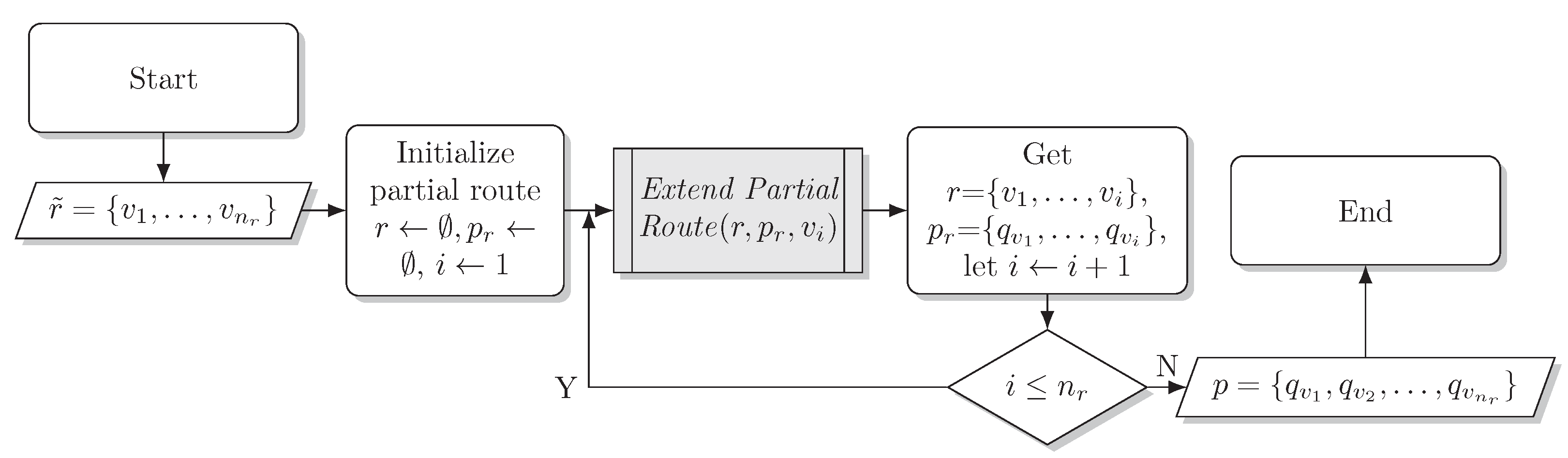
As shown in Figure 1, given a route $r=\{v_1,v_2,\dots ,v_{n_r}\}$, the exact method Optimal Pattern $\left(r\right)$ considers each station’s pickup/delivery quantity case by case from $v_1$ to $v_{n_r}$. Each time the paritial route r with pattern $p_r$ is extended to a new station $\delta \in r$, the sub-procedure Extend Paritial Route $(r,p_r,\delta )$ is executed to obtain the optimal pickup and delivery pattern of the new partial route, achieving $v_k$.

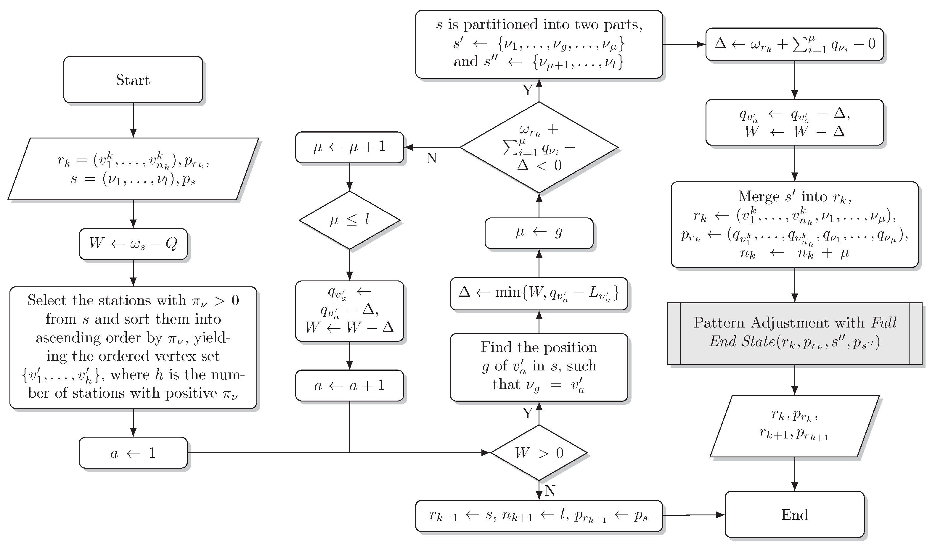
Figure 2 is the flow diagram of the sub-procedure Extend Paritial Route $(r,p_r,\delta )$. In each execution, firstly input the partial route and its compatible pickup and delivery pattern with the subroute partition information $r=(r_1,\dots ,r_k,s)$, $p_r=(p_{r_1},\dots ,p_{r_k},p_s)$ as well as the newly reached station $\delta$. Then, initialize the pickup/delivery quantity of the newly reached station $\delta$ to its upper or lower bound ($q_{\delta }\leftarrow U_{\delta }\mathrm{or}{L}_{\delta }$) according to its dual price ${\pi }_{\delta }$. Add $\delta$ to the end of the partial route, namely, the end of the route segment, and check whether the vehicle capacity constraint (37) at station $\delta$ is satisfied. Once violated, we will adjust the pickup and delivery pattern of the route segment; otherwise, terminate the sub-procedure.

In the case that the violation is an excess of Q, a new subroute with full end state would arise after the execution of the sub-procedure Pattern Adjustment with Full End State $(r_k,p_{r_k},s^{″},p_{s^{″}})$ shown in Figure 3. We should first check whether the end state of the route segment s is the same as the last subroute $r_k$. If so, the last subroute $r_k$ would combine with the route segment s, becoming a new route segment $s\leftarrow r_k\cup s$, and the number of subroutes would drop by one, $k\leftarrow k-1$. Then, the new route segment s and the last subroute $r_k$ with their pickup and delivery patterns are inputted into the the sub-procedure Pattern Adjustment with Full End State $(r_k,p_{r_k},s,p_s)$. Otherwise, the last subroute $r_k$ and the route segment s with their patterns will be inputted into the sub-procedure directly.

In the case that the violation is a vehicle load less than zero, a new subroute with empty end state would arise after the execution of the sub-procedure Pattern Adjustment with Empty End State $(r_k,p_{r_k},s^{″},p_{s^{″}})$ shown in Figure 4. Similar to the previous case, we check the end states first to confirm whether to combine the last subroute and the route segment and then input the last subroute and the route segment into the sub-procedure Pattern Adjustment with Empty End State $(r_k,p_{r_k},s,p_s)$.

In the sub-procedure Pattern Adjustment with Full End State $(r_k,p_{r_k},s,p_s)$ in Figure 3, calculate the excess quantity W. Firstly, select and sort the vertices in the route segment, and then decrease the pickup/delivery quantity of the vertex to its lower bound case by case according to this sequence until $W=0$ Each time a vertex’s quantity is reduced, check whether the vehicle capacity constraints from this vertex to the end of the segment 0 ≤ ω_rk + ${\sum }_{i=1}^{\mu }$ q_vi − Δ ≤ Q, μ = {g,…,l} are satisfied. If not, the route segment is partitioned into two parts, the previous one has become a subroute, and the latter, still with excess quantity, should be handled by the Pattern Adjustment with Full End State (r_k, p_rk, s, p_s) again. The sub-procedure Pattern Adjustment with Full End State (r_k, p_rk, s, p_s) in Figure 4 is the same way.

4.1.2. Exact and Heuristic Label-Setting

Ding et al. [41] developed a Label-Setting algorithm embedded with the exact method for optimal pickup and delivery pattern, which is capable of exactly solving the pricing subproblem (23)–(34).

The label is defined as $E=(v,r,p_r,\tau ,\xi ,\eta )$, corresponding to the elementary (partial) route $r=\{v_1,\dots ,v_j\}$ ending up with vertex $v=v_j$, and the optimal pickup and delivery pattern $p_r=\{q_{v_1},\dots ,q_{v_j}\}$, obtained by the exact method described above. Moreover,

• $\tau$ is the total time consumed along (partial) route r, including the travel time and the service time, $\tau =\tau (r,p_r)={\sum }_{i=1}^{j-1}{t}_{v_i,v_{i+1}}+\gamma {\sum }_{q\in p_r}\left|q\right|$,
• $\xi$ is the reduced cost of (partial) route r with the compatible pickup and delivery pattern $p_r$, including the travel cost and the dual variable cost with respect to $p_r$, $\xi =\xi (r,p)={\sum }_{i=1}^{j-1}{\widehat{c}}_{v_i,v_{i+1}}-{\sum }_{i=1}^j{\pi }_{v_i}{q}_{v_i}-\beta$, and
• $\eta$ is the vehicle load at vertex v.

Hence, the initial label at vertex 0 is defined as $E_0=(0,r_0,p_{r_0},{\tau }_0,{\xi }_0,{\eta }_0)$ = $(0,\{0\},\{0\},$ $0,0,0)$. A label $E=(v,r,p_r,\tau ,\xi ,\eta )$ can be extended to vertex $v^{\prime },v^{\prime }\in V\setminus r$ along arc $(v,v^{\prime })\in A$, generating a new label $E^{\prime }=(v^{\prime },r^{\prime },p_{r^{\prime }},{\tau }^{\prime },{\xi }^{\prime },{\eta }^{\prime })$. The extension functions are

• $(r^{\prime },p_{r^{\prime }})=$Extend Partial Route$(r,p_r,v^{\prime })$ in Figure 2, where $r=\{v_1,\dots ,v_j\}$, $v=v_j$, $p_r=\{q_{v_1},\dots ,q_{v_j}\}$, $v_{j+1}=v^{\prime }$, $r^{\prime }=\{v_1,\dots ,v_j,v_{j+1}\}$ and $p_{r^{\prime }}=\{q_{v_1}^{\prime },\dots ,q_{v_j}^{\prime },q_{v_{j+1}}^{\prime }\}$,
• ${\tau }^{\prime }=\tau (r^{\prime },p_{r^{\prime }})$,
• ${\xi }^{\prime }=\xi (r^{\prime },p_{r^{\prime }})$,
• ${\eta }^{\prime }={\sum }_{q\in p_{r^{\prime }}}q$.

The proposed dominance rule is shown as follows. If E dominates $E^{\prime }$, then the following conditions hold:

• $v=v^{\prime }$,
• $\tau \le {\tau }^{\prime }$,
• $\xi \le {\xi }^{\prime }$,
• $\eta ={\eta }^{\prime }$,
• $r\subseteq r^{\prime }$.

The objective function of the pricing subproblem (23) shows that the solution of the pricing subproblem is seriously affected by the term ${\sum }_{i\in V_C}{\pi }_i{q}_i$. Therefore, to speed up the exact label-setting algorithm, we use a heuristic strategies that eliminate some stations with the minimal ${\pi }_i{q}_i$. Each time the heuristic label-setting (HLS) is used, all the stations are sorted in descending order according to the value of ${\pi }_i{q}_i,i\in V_C$. Then, a percentage of stations at the top of the list will remain, and the rest are rejected from the graph $G=(V,A)$. The rejection procedure is executed at the beginning of the HLS. The HLS can be executed multiple times with different parameters of the remaining percentage from small to large. The suitable times and parameters of the remaining percentage will be explored in Section 5.1.

4.1.3. Tabu Search Column Generator

It is unnecessary to solve the pricing subproblem optimally in each column generation iteration. It is more efficient to find a negative reduced cost column heuristically. Thus, a tabu search (TS) column generator is proposed in this section to accelerate the column generation process. The TS method chooses the stations and determines their order, while the exact method in Figure 1 determines the compatible pickup and delivery pattern.

Consider the following notations.

• S: the set of routes with their compatible pickup and delivery patterns with negative reduced cost found by the TS method.
• $maxCol$: the maximum number of the routes in S.
• $R_B$: the set of routes with their compatible pickup and delivery patterns associated with the basic columns of the RLMP in current column generation iteration.
• $maxIter$: the maximum number of TS iterations for each basic column in $R_B$.
• $tabuSize$: the maximum size of the tabu list.

TS begins with the set of basic columns $R_B$; namely, the columns with zero reduced cost. Then, it is independently executed on each column in $R_B$. In each execution, two types of neighborhoods of the column are explored by applying REMOVE and ADD $maxIter$ times.

• REMOVE: select a station $v\in r$, remove it from r, and calculate the compatible optimal pickup and delivery pattern by the exact method $Optimal Pattern\left(r\right)$ in Figure 2.
• ADD: select a station $v\in V_C\setminus r$, add it to r, and calculate the compatible optimal pickup and delivery pattern by the exact method $Optimal Pattern\left(r\right)$, finding the cheapest ADD.

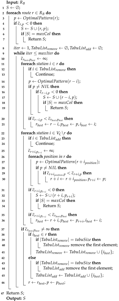
The procedure terminates until the size of the set S reaches $maxCol$. Algorithm 1 shows the detailed procedure of the Tabu Search Column Generator.

4.2. Cutting

This section extends three types of non-robust valid inequalities for the HFMDSBRP-SD, namely, the subset-row inequality, the strong minimum number of vehicles inequality, and the elementary inequality. These inequalities are all defined on the variables ${\vartheta }_{r,p}$ in the MP. Thus, they are non-robust valid inequalities that will change the structure of the pricing subproblems and increase the problem complexity. However, the non-robust valid inequalities present a better performance of tightening the lower bound of the MP.

4.2.1. Subset-Row Inequalities

The subset-row (SR) inequalities were proposed by Jepsen et al. [42], corresponding to a subset of the rank-1 Chvátal-Gomory inequalities. Given a subset of stations $C\subseteq V_C$, the SR inequalities can be expressed as

$$\sum _{k\in K}\sum _{r\in R_k}\sum _{p\in P_r}\lfloor \rho \sum _{i\in C}{a}_{i,r,p}^F\rfloor {\vartheta }_{r,p}\le \lfloor \rho \left|C\right|\rfloor \forall C\subseteq V_C$$

(39)

where the binary parameter $a_{i,r,p}^F=1$ if the pickup/delivery demand of station i is fully satisfied in pattern p for route r, namely, $q_i={\mathcal{D}}_i$, is the subset of the station set, and $\rho =1/h,h\in \{1,\dots ,|C\left|\right\}$.

Varying the cardinality of C and the value of $\rho$ yields four types of SR inequalities, as follows.

• 3-SR: the SR inequalities with $\left|C\right|=3\mathrm{and}\rho =1/2$.
• 4-SR: the SR inequalities with $\left|C\right|=4\mathrm{and}\rho =2/3$.
• 5,1-SR: the SR inequalities with $\left|C\right|=5\mathrm{and}\rho =1/3$.
• 5,2-SR: the SR inequalities with $\left|C\right|=5\mathrm{and}\rho =1/2$.

Preliminary test results showed that the SR inequalities for subset C with $\left|C\right|\ge 3$ are rarely violated in the HFMDSBRP-SD. Therefore, only 3-SR inequalities are considered in this paper. The 3-SR inequalities are separated by complete enumeration.

Algorithm 1: Tabu Search Column Generator.

Define ${\delta }_C$ as the dual variables of the 3-SR inequalities. The reduced cost of variable ${\vartheta }_{r,p}$ becomes

$${\overline{c}}_{r,p}=\sum _{(i,j)\in A}(c_{i,j}-{\alpha }_i)x_{i,j}-\sum _{i\in V_C}{\pi }_i{q}_i-{\beta }_{l,h}-\sum _{C\subseteq V_C:\left|C\right|=3}\lfloor \rho \sum _{i\in C}{a}_{i,r,p}^F\rfloor {\delta }_C$$

(40)

In the three column generators used in this paper, the pickup and delivery pattern will change with the extension of the partial route. Therefore, the term ${\sum }_{C\subseteq V_C:\left|C\right|=3}\lfloor \rho {\sum }_{i\in C}{a}_{i,r,p}^F\rfloor {\delta }_C$ will be calculated when the route extends to the depot.

4.2.2. Strong Minimum Number of Vehicles Inequalities

Let $Q_{max}={max}_{h\in H}\left\{Q_h\right\}$, and let $\overline{V}$ be the set of stations, such that the station $i\in V_C$ and $|{\mathcal{D}}_i|\le Q_{max}$. The strong minimum number of vehicles (SMV) inequalities can be expressed as

$$\sum _{k\in K}\sum _{r\in R_k}\sum _{p\in P_r}(2a_{i,r,p}^F+a_{i,r,p}^{SZ}){\vartheta }_{r,p}\ge 2,\forall i\in \overline{V}$$

(41)

where the binary parameter $a_{i,r,p}^F=1$ if the pickup/delivery demand of station i is fully met in pattern p for route r, and the binary parameter $a_{i,r,p}^{SZ}=1$ if a split pickup/delivery or a zero pickup/delivery is performed at station i in pattern p for route r.

Define ${\zeta }_i$ as the dual variables of the SMV inequalities. The reduced cost of variable ${\vartheta }_{r,p}$ becomes

$$\begin{array}{c}\hfill {\overline{c}}_{r,p}=\sum _{(i,j)\in A}(c_{i,j}-{\alpha }_i)x_{i,j}-\sum _{i\in V_C}{\pi }_i{q}_i-{\beta }_{l,h}-\sum _{C\subseteq V_C:\left|C\right|=3}\lfloor \rho \sum _{i\in C}{a}_{i,r,p}^F\rfloor {\delta }_C-\sum _{i\in \overline{V}}(2a_{i,r,p}^F+a_{i,r,p}^{SZ}){\zeta }_i\end{array}$$

(42)

The same is true of the SR inequalities; the dual prices of SMV inequalities is calculated when the route extends to the depot.

4.2.3. Elementary Inequalities

The elementary inequalities were first introduced by Balas [43], inspired by the fact that if route r is used, for a node i not visited by route r, the route visiting i cannot visit any node visited by route r; otherwise, at least one node visited by route r will be visited twice.

Pecin et al. [44] developed enhanced elementary inequalities proven to dominate the elementary inequalities proposed by Balas [43], which is also a subset of the rank 1 Chvátal–Gomory inequalities. Given a station subset $C\subset V_C$, and a station $i\in V_C\setminus C$, considering two multipliers $p_i^C=\left(\right|C|-1)/\left|C\right|$ and $p_j^C=1/\left|C\right|,j\in C$, the enhanced elementary inequalities are expressed as

$$\sum _{k\in K_h}\sum _{r\in R_k}\sum _{p\in P_r}\lfloor p_i^C{a}_{i,r,p}^F+\sum _{j\in C}{p}_j^C{a}_{j,r,p}^F\rfloor {\vartheta }_{r,p}\le 1\forall C\subset V_C,i\in V_C\setminus C.$$

(43)

A local search separation algorithm is used to find the violated elementary inequalities. The local search separation algorithm requires the following notations.

• R: the set of all feasible routes, $R={\cup }_{k\in K}{R}_k$.
• $\Omega$: the set of all routes with their compatible pickup and delivery patterns, $\Omega =\left\{(r,p)\right|r\in R,p\in P_r\}$.
• $\Omega \left(i\right)$: given a station $i\in V_C$, $\Omega \left(i\right)$ is the subset of $\Omega$ such that a full pickup/delivery is performed at station i in pattern p for route r for each $(r,p)\in \Omega \left(i\right)$.
• ${\Omega }^{\perp }\left(i\right)=\Omega \setminus \Omega \left(i\right)$.
• $V(r,p)$: the set of stations visited by r with pattern p and receiving a full pickup/delivery.
• $W\left(i\right)={\cup }_{(r,p)\in \Omega \left(i\right)}V(r,p)$.

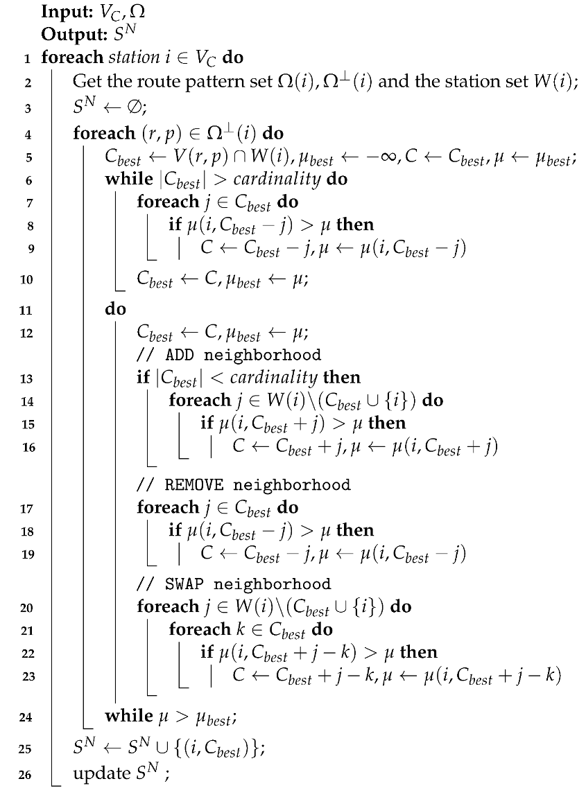
The local search is executed for each pair of station $i\in V_C$ and $(r,p)\in {\Omega }^{\perp }\left(i\right)$, as shown in Algorithm 2.

Algorithm 2: Local Search Separation Algorithm for Elementary Inequalities.

Define ${\sigma }_{i,C}$ as the dual variables of the elementary inequalities. The reduced cost of variable ${\vartheta }_{r,p}$ becomes

$$\begin{array}{cc}\hfill {\overline{c}}_{r,p}=& \sum _{(i,j)\in A}(c_{i,j}-{\alpha }_i)x_{i,j}-\sum _{i\in V_C}{\pi }_i{q}_i-{\beta }_{l,h}-\sum _{C\subseteq V_C:\left|C\right|=3}\lfloor \rho \sum _{i\in C}{a}_{i,r,p}^F\rfloor {\delta }_C\hfill \\ \hfill & -\sum _{i\in \overline{V}}(2a_{i,r,p}^F+a_{i,r,p}^{SZ}){\zeta }_i-\sum _{C\subseteq V_C:\left|C\right|\le cardinality}\sum _{i\in V_C\setminus C}\lfloor p_i^C{a}_{i,r,p}^F+\sum _{j\in C}{p}_j^C{a}_{j,r,p}^F\rfloor {\sigma }_{i,C}\hfill \end{array}$$

(44)

The same is true for the SR inequalities; the dual prices of elementary inequalities are calculated when the route extends to the depot.

4.2.4. Cutting Strategies

In our proposed BPC algorithm, the three types of valid inequalities are separated and added to the RLMP only in the branch-and-bound nodes with depths less than three. The preliminary test results show that this is better than the strategies with depths less than 5 and 10. There are two types of cutting strategies.

• All valid inequalities are separated and added to the RLMP in each iteration.
• The valid inequalities are ordered based on the separating time. Then, only one type of valid inequality is sought and added to the RLMP in an iteration. It turns to the following type of valid inequalities until this type of valid inequality cannot be found anymore. It terminates until the last type of valid inequality cannot be found.

The two cutting strategies will be tested and compared in Section 5.2.

4.3. Branching Strategies

To retain the structures of three column generators, branching on the decision variables ${\vartheta }_{r,p}$ is not feasible. Hence, we use four types of branching strategies, namely, branching on (1) the number of each type of vehicle used, (2) the number of times each station is visited, (3) the number of times each arc in A is visited, and (4) the number of times two consecutive arcs are visited. Note that the last branching strategy will change the structure of the column generator. However, it is rarely used in the solution process and is obligatory to guarantee integrality.

5. Computational Experiments

The instances used to test the proposed BPC algorithm are generated based on the instance generation scheme in Hernandez-Perez and Salazar-Gonzalez [45] and Chemla et al. [11]. The stations are randomly located in the square $[-500,500]\times [-500,500]$. If one only considers one depot, it is located at $(0,0)$. If one considers two depots, they locate at $(-212,0)$ and $(212,0)$. The demand of each customer is randomly selected from $[-10,10]$. We generate three instance classes with $n=10,20,30$, named as $n10,n20,n30$, respectively. Each class has 10 instances. Define four vehicle capacities $Q=8,10,12,15$. Three cases are considered individually for $n10,n20,n30$ instance classes. Case 1: one depot and one repositioning vehicle with $Q=8,10,12,15$, Case 2: one depot and two vehicles with the capacity combination $(8,12),(8,15),(10,12),(10,15)$, and Case 3: two depots and one vehicle with $Q=8,10,12,15$. Thus, the total number of instances is 360.

All tests are coded in C++ and performed on a Windows PC equipped with 224 GB of RAM and an Intel(R) Xeon(R) Gold 6142 CPU @ 2.60GHz. All the MPs are solved by the CPLEX solver. A time limit of two hours is set for each test. The computational experiments mainly focus on comparing the column generator results, the valid inequalities results, and the integer solution results.

5.1. Column Generator Results

Firstly, we conduct the experiments for the HLS parameter selection. The HLS parameter is the percentage of the stations that remain in the label-setting algorithm. The computational experiments are conducted on the RLMP at the root node of the branch-and-bound tree. Twenty instances are selected. The first 10 instances belong to the $n20$ instance class with one depot and one vehicle with $Q=10$, expressed as $n10$ in

Table 1. The HLS parameter comparison on the average time in seconds to solve RLMP at the root branch-and-bound node.

	Column	Parameters of HLS
	Generators	0.70	0.75	0.80	0.85	0.90	0.60	0.65	0.70	0.60	0.65	0.70	0.60	0.65	0.70
							+0.80	+0.80	+0.80	+0.85	+0.85	+0.85	+0.90	+0.90	+0.90
n20	HLS + ELS	7.5	9.1	7.4	6.7	8.8	5.5	4.1	6.1	5.3	5.1	5.4	7.8	3.9	7
	TS + HLS + ELS	2.026	1.116	0.417	0.846	1.765	1.01	0.441	0.729	0.629	0.508	0.531	0.612	0.793	0.615
n30	HLS + ELS	137.3	57.8	62.2	72.6	134.5	51.7	55.8	57	53.4	50.9	58.3	63.3	56	60.2
	TS + HLS + ELS	11.673	16.4	20.358	20.553	27.596	7.695	11.91	10.56	17.394	14.606	12.656	21.765	19.751	12.561

. The last 10 instances belong to the $n30$ instance class with one depot and one vehicle with $Q=10$, expressed as $n20$ in Table 1. Then, we consider four column-generator-application strategies, namely one-phrase HLS + ELS, two-phrase HLS + ELS, TS + one-phrase HLS + ELS, and TS + two-phrase HLS + ELS. For the one-phrase HLS, five parameters are considered, i.e., 0.70, 0.75, 0.80, 0.85, and 0.9. For the two-phrase HLS, nine parameter combinations are considered, i.e., 0.60 + 0.80, 0.65 + 0.80, 0.70 + 0.80, 0.60 + 0.85, 0.65 + 0.85, 0.70 + 0.85, 0.60 + 0.90, 0.65 + 0.90, and 0.70 + 0.90.

Table 1 reports the average time taken to solve the RLMP at the root branch-and-bound node on $n20,n30$ instance classes in four column-generator-application strategies. The results indicate that the column-generator-application strategy with TS is much better than that without TS, and the efficiency and robustness of the average time for the TS + two-phrase HLS + ELS strategy are the best among the four strategies. Therefore, the TS + 2-phrase HLS + ELS is applied in the following computational experiments, and the parameter combination 0.65 + 0.80 is selected.

Table 2. Root Node RLMP Results.

	ELS			HLS + ELS			TS + HLS + ELS
	nIt	Obj	Time (s)	nIt	Obj	Time (s)	nIt	Obj	Time (s)
n20q10A	22	8676.28	0.515	25	8334.45	0.312	26	8334.45	0.337
n20q10B	58	6950.35	5.891	65	6950.58	2.33	69	6950.31	4.145
n20q10C	52	5592.62	6.204	51	5592.62	1.65	63	5592.62	2.325
n20q10D	68	5734.84	30.17	76	5738.91	12.089	85	5685.19	11.391
n20q10E	48	7959.58	2.674	47	7952.87	1.217	56	7952.87	2.074
n20q10F	68	5734.84	29.802	76	5738.91	11.926	85	5685.19	11.055
n20q10G	57	5617.24	7.001	54	5607.22	1.184	80	5625.99	4.861
n20q10H	53	6257.81	40.164	57	6257.81	10.783	61	6257.81	12.656
n20q10I	44	7202.03	3.438	61	7202.03	1.414	54	7202.03	1.218
n20q10J	51	7870.32	4.497	55	7870.32	2.236	54	7870.32	1.132
n30q10A	63	10,694.8	55.596	81	10,694.8	31.039	74	10,694.8	11.439
n30q10B	86	9946.06	103.328	108	9946.06	39.183	107	9920.41	35.379
n30q10C	107	7561.86	310.105	132	7515.7	83.024	135	7561.86	87.734
n30q10D	89	10,495.2	110.248	86	10,471.8	29.721	111	10,466	24.795
n30q10E	104	7388.76	201.02	107	7388.76	92.367	120	7388.76	77.253
n30q10F	97	6977.04	345.708	114	6982.64	162.821	122	6978.15	93.857
n30q10H	96	9313.44	211.312	105	9308.33	64.601	121	9319.82	60.363
n30q10I	74	8003.23	56.51	83	7995.36	40.054	69	7992.55	8.049
n30q10J	69	9627.54	74.484	89	9629.8	18.26	101	9654.02	20.394

displays the number of column generation iterations (nIt) the objective value (Obj) and the total computational time in seconds to solve the RLMP in the root branch-and-bound node (Time) on the $n20,n30$ instance classes with one depot and one vehicle with $Q=10$. As shown, in the $n20$ instance class, HLS + ELS provides the minimal average computational time because label setting can solve the small-scale problem more efficiently than TS. However, the results on $n20,n30$ prove the effectiveness of TS. Although the HLS and TS increase the number of column generation iterations, the total computational time is reduced.

5.2. Valid Inequality Results

To evaluate the performance of various valid inequalities, we conduct the computational experiments on $n20,n30$ instance classes with one depot and one vehicle with $Q=10$ to get (1) The lower bounds obtained at root branch-and-bound node without any valid inequality $\left(LB\right)$; (2) The lower bounds at root node achieved by adding 3-SR inequalities $\left(L{B}_{3\text{-}SR}\right)$, SMV inequalities $\left(L{B}_{SMV}\right)$, and elementary inequalities $\left(L{B}_E\right)$ individually; (3) The lower bounds at root node achieved by adding two or three types of valid inequalities (SVM + E, SVM + 3-SR, 3-SR + EC, and SMV + 3-SR + E) in cutting strategy 1 and 2, as described in Section 4.2.4; and (4) the upper bound $\left(UB\right)$.

Table 3. Gaps Improved by Various Valid Inequalities.

Inst Class	3-SR	SMV	E	Cutting Strategy	SMV + E	SMV + 3-SR	3-SR + E	SMV + 3-SR + E
n20	15.20%	47.43%	16.16%	Strategy 1	57.03%	58.16%	15.84%	61.38%
				Strategy 2	36.26%	43.68%	4.06%	57.26%
n30	5.66%	57.56%	3.70%	Strategy 1	59.20%	60.08%	5.05%	62.78%
				Strategy 2	6.21%	48.17%	39.29%	58.42%

reports the average gap improved by various inequalities; that is, ($L{B}_x-LB$)/($UB-LB$), where x refers to any valid inequalities or combinations.

As shown, the SMV inequalities are the most effective valid inequalities among the three types. Moreover, for the most valid inequality combinations, the average gaps in cutting strategy 1 are better than those in cutting strategy 2. The average gap improved by SMV + 3-SR + E in Strategy 1 is the best in both $n20,n30$ instance classes. Therefore, all three types of valid inequalities and cutting strategy 1 are used in the following computational experiments.

5.3. Integer Solution Results

Finally, the computational experiments are conducted on all instances.

Table 4. Summary of the Integer Solution Results on the $n10$ Instances.

Inst Class	NB dpt	NB veh	Q	NB Inst	NB Solved	LB	LB_cut	IP	LB Time	Root Time	IP Time	Cut Time	Tree Size	nSMV	n3SR	nE	nSplits
$n10$	1	1	8	10	10	4686.1	4850.5	4989.9	0	0	0.1	0	18.8	1.1	0.5	10.2	0.9
$n10$	1	1	10	10	10	4225.2	4411.3	4499.3	0	0	0	0	4	1.1	0.4	10.4	0.6
$n10$	1	1	12	10	10	4168.9	4192.1	4310.7	0	0	0	0	3	0.4	0	2.9	0.1
$n10$	1	1	15	10	10	4109.6	4169.8	4242.7	0	0	0	0	1.6	0.7	0	2.7	0.1
$n10$	1	2	8, 12	10	10	5379.7	5686.7	5774.3	0	0	0	0	8.2	1.9	1.3	10.3	0.3
$n10$	1	2	8, 15	10	10	5437.6	5875.4	5908.5	0	0	0	0	3.8	1.3	1.1	11.9	0.3
$n10$	1	2	10, 12	10	10	5446.6	5694.7	5824.8	0	0	0	0	5.8	1.2	1.6	10.6	0.1
$n10$	1	2	10, 15	10	10	5490.5	5844.8	5916.4	0	0	0	0	3.4	1.1	1.7	11.1	0.1
$n10$	2	1	8	10	8	4462.73	4626.7	4754.06	0.094	0.115	0.708	0.101	21.25	0.625	2.125	10.25	0.75
$n10$	2	1	10	10	10	4492.6	4823.3	4934.3	0	0	0	0	8.8	1.8	0.9	11.8	1.7
$n10$	2	1	12	10	10	4687.9	4875	4993.8	0	0	0.1	0	7.8	1.2	0.8	7.4	0.3
$n10$	2	1	15	10	10	4942.3	5100.3	5193.5	0	0	0	0	4.4	1	2.9	5.9	0.2

,

Table 5. Summary of the Integer Solution Results on the $n20$ Instances.

Inst Class	NB dpt	NB veh	Q	NB Inst	NB Solved	LB	LB_cut	IP	LB Time	Root Time	IP Time	Cut Time	Tree Size	nSMV	n3SR	nE	nSplits
$n20$	1	1	8	10	10	8026.5	8098.3	8311.1	5.8	9.8	101.9	4.5	140.4	3.7	12.8	23.9	3.8
$n20$	1	1	10	10	10	6715.2	7004.8	7417.6	3.8	23.8	87.6	3.1	30	7	27.1	17.9	1.8
$n20$	1	1	12	10	10	6464.7	6672.7	6983.4	7.1	10.6	27.8	0.3	10.4	4	14.5	20.2	1.8
$n20$	1	1	15	10	10	6271.7	6363.1	6472.9	6	8.8	12.8	0	5.4	2.1	13.4	14	0.3
$n20$	1	2	8, 12	10	10	7869.8	8132.8	8243.7	24.9	33.5	91.6	3.7	18.8	4.7	24.2	16	1
$n20$	1	2	8, 15	10	10	8072.7	8332.4	8311	33.1	62.6	79.7	0.7	3.6	3.2	22	16	1.5
$n20$	1	2	10, 12	10	10	7910.4	8151.2	8354.1	23.8	40	81.3	1.8	15.8	4.7	25.5	20	1.7
$n20$	1	2	10, 15	10	10	8076.6	8305.3	8387.8	18.8	77.1	112	0	5.4	2.1	22.6	20	1.3
$n20$	2	1	8	10	10	7300.2	7484.4	7620.8	61.9	99.4	1167.8	27.1	82.8	10.8	76.6	21.1	4.9
$n20$	2	1	10	10	10	6330.9	6666.4	6969.7	52	115.8	479.4	20.31	21.8	8.3	65.9	18	3.4
$n20$	2	1	12	10	10	6430	6658.7	6754.9	96.1	165.1	331.7	3.9	8.2	5.1	43.6	16.1	2.4
$n20$	2	1	15	10	10	6577.8	6770.9	6859.1	106.3	136.7	221.9	3.4	6.2	3.1	36.3	12	0.7

and

Table 6. Summary of the Integer Solution Results on the $n30$ Instances.

Inst Class	NB dpt	NB veh	Q	NB inst	NB Solved	LB	LB_cut	IP	LB Time	Root Time	IP Time	Cut Time	Tree Size	nSMV	n3SR	nE	nSplits
$n30$	1	1	8	10	4	10,140.3	10,260.57	10,731.7	69.7	101.9	824	18.53	65	11.25	54.25	22	8.5
$n30$	1	1	10	10	10	8836.8	9178.1	9610.3	55.9	106	1247.4	39.7	63.6	10.1	83.1	20	4.2
$n30$	1	1	12	10	10	8259.75	8563	8854	84.1	131.8	467.4	5.25	11	8.125	42.5	20.1	3.63
$n30$	1	1	15	10	10	8345.9	8557.8	8716.6	159.7	237.5	800.5	7.7	20	6.7	42.5	20	2.1
$n30$	1	2	8, 12	10	7	10,005.1	10,538.4	10,936.9	560	824.9	2654.7	52.57	32.43	18.14	110.4	22.1	2.86
$n30$	1	2	8, 15	10	9	10,301.3	10,741.3	11,028.3	711.6	1472.8	4079.9	41.7	24.56	14.67	111.4	20	4.56
$n30$	1	2	10, 12	10	8	10,176.4	10,698.1	11,174.9	498.5	681.6	3236.8	72.125	37.75	15.75	120.8	20.4	2
$n30$	1	2	10, 15	10	8	10,342.8	10,745.9	11,059.8	728.1	1359.5	4029.6	48.5	29.25	12.13	114.4	20	2.1
$n30$	2	1	8	10	0	-	-	-	-	-	-	-	-	-	-	-	-
$n30$	2	1	10	10	0	-	-	-	-	-	-	-	-	-	-	-	-
$n30$	2	1	12	10	0	-	-	-	-	-	-	-	-	-	-	-	-
$n30$	2	1	15	10	0	-	-	-	-	-	-	-	-	-	-	-	-

report the summary of the results, including the number of depots (NB dpt), the number of repositioning vehicles (NB veh), the capacity of each type of repositioning vehicle (Q), the number of instances in the instance class (NB inst), the number of solved instances (NB solved), and the following averages over the solved instances: the lower bound achieved by column generation at root branch-and-bound node (LB), the lower bound obtained by adding valid inequalities at root branch-and-bound node (LB_cut), the integer programming solution (IP), the time in seconds for LB (LB time), the time in seconds for solving the root branch-and-bound node (Root time), the time in seconds for IP (IP time), the time in seconds for separating valid inequalities (cut time), the number of nodes in the branch-and-bound tree (Tree size), the total number of SMV inequalites (nSMV), the total number of 3-SR inequalities (n3SR), the total number of elementary inequalities (nE), and the number of split pickup/delivery (nSplits). The detailed computational results are reported in the

Table A1. Integer Solution Results on the n10 Instances with One Depot and One Repositioning Vehicle.

Inst Class	NB dpt	NB veh	Q	LB	LB_cut	IP	LB Time	Root Time	IP Time	Cut Time	Tree Size	nSMV	n3SR	nE	nSplits
$n10$_1	1	1	8	5081.87	5081.87	5413.39	0.035	0.044	0.092	0.012	11	0	0	20	1
$n10$_2	1	1	8	7063.97	7063.97	7063.97	0.005	0.005	0.005	0	1	0	0	0	1
$n10$_3	1	1	8	4464.4	4464.4	4464.4	0.046	0.046	0.046	0	1	0	0	0	0
$n10$_4	1	1	8	3576.35	3618.1	3671.19	0.026	0.042	0.067	0.012	5	1	1	20	0
$n10$_5	1	1	8	6200.4	6454.08	7098.91	0.009	0.013	1.215	0.19	145	3	0	7	3
$n10$_6	1	1	8	3760.96	4087.61	4227.58	0.018	0.031	0.057	0.01	5	1	1	17	1
$n10$_7	1	1	8	3045.64	3045.64	3045.64	0.045	0.045	0.045	0	1	0	0	0	0
$n10$_8	1	1	8	4863.58	4907.06	4924.01	0.015	0.049	0.1	0.004	3	2	0	14	2
$n10$_9	1	1	8	4207.98	4213.32	4219.26	0.036	0.065	0.102	0.006	3	1	3	14	0
$n10$_10	1	1	8	4602.9	5573.33	5775.83	0.024	0.04	0.173	0.016	13	3	0	10	1
$n10$_1	1	1	10	4924.65	4939	4939	0.069	0.111	0.111	0.002	1	1	0	16	1
$n10$_2	1	1	10	6067.46	6067.46	6067.46	0.016	0.017	0.017	0	1	0	0	0	0
$n10$_3	1	1	10	3279.73	3279.73	3279.73	0.055	0.055	0.055	0	1	0	0	0	0
$n10$_4	1	1	10	3415.91	3645.05	3819.28	0.021	0.132	0.226	0.032	9	3	1	20	1
$n10$_5	1	1	10	5639.99	5903.12	6239.81	0.005	0.009	0.043	0.008	11	2	0	10	3
$n10$_6	1	1	10	3563.83	3604.01	3673.52	0.016	0.025	0.04	0.003	3	1	0	20	0
$n10$_7	1	1	10	3045.64	3045.64	3045.64	0.058	0.058	0.058	0	1	0	0	0	0
$n10$_8	1	1	10	4381.62	4381.62	4381.62	0.019	0.019	0.019	0	1	0	0	0	0
$n10$_9	1	1	10	4209.83	4216.8	4219.26	0.073	0.086	0.129	0.006	3	0	3	18	0
$n10$_10	1	1	10	3730.52	5035	5332.39	0.022	0.063	0.141	0.024	9	4	0	20	1
$n10$_1	1	1	12	4917.48	4917.48	4917.48	0.022	0.022	0.022	0	1	0	0	0	0
$n10$_2	1	1	12	6067.46	6067.46	6067.46	0.03	0.038	0.038	0	1	0	0	0	0
$n10$_3	1	1	12	3279.73	3279.73	3279.73	0.04	0.04	0.04	0	1	0	0	0	0
$n10$_4	1	1	12	3357.22	3357.22	3357.22	0.01	0.01	0.01	0	1	0	0	0	0
$n10$_5	1	1	12	5602.72	5815.83	6892.57	0.005	0.01	0.049	0.009	17	3	0	9	1
$n10$_6	1	1	12	3523.65	3523.65	3523.65	0.008	0.008	0.008	0	1	0	0	0	0
$n10$_7	1	1	12	3045.64	3045.64	3045.64	0.043	0.043	0.043	0	1	0	0	0	0
$n10$_8	1	1	12	4241.95	4260.85	4369.08	0.013	0.021	0.047	0.007	5	1	0	20	0
$n10$_9	1	1	12	4130.27	4130.27	4130.27	0.07	0.07	0.07	0	1	0	0	0	0
$n10$_10	1	1	12	3528.21	3528.21	3528.21	0.032	0.032	0.032	0	1	0	0	0	0
$n10$_1	1	1	15	4917.48	4917.48	4917.48	0.032	0.032	0.032	0	1	0	0	0	0
$n10$_2	1	1	15	6067.46	6067.46	6067.46	0.019	0.021	0.021	0	1	0	0	0	0
$n10$_3	1	1	15	3279.73	3279.73	3279.73	0.048	0.048	0.048	0	1	0	0	0	0
$n10$_4	1	1	15	3357.22	3357.22	3357.22	0.011	0.011	0.011	0	1	0	0	0	0
$n10$_5	1	1	15	5203.5	5670.76	6226.45	0.009	0.018	0.022	0.002	3	4	0	7	1
$n10$_6	1	1	15	3523.65	3523.65	3523.65	0.016	0.016	0.016	0	1	0	0	0	0
$n10$_7	1	1	15	3045.64	3045.64	3045.64	0.039	0.039	0.039	0	1	0	0	0	0
$n10$_8	1	1	15	4047.05	4182.46	4355.97	0.007	0.026	0.052	0.009	5	3	0	20	0
$n10$_9	1	1	15	4130.27	4130.27	4130.27	0.07	0.07	0.07	0	1	0	0	0	0
$n10$_10	1	1	15	3528.21	3528.21	3528.21	0.047	0.047	0.047	0	1	0	0	0	0

,

Table A2. Integer Solution Results on the n10 Instances with One Depot and Two Repositioning Vehicles.

Inst Class	NB dpt	NB veh	Q	LB	LB_cut	IP	LB Time	Root Time	IP Time	Cut Time	Tree Size	nSMV	n3SR	nE	nSplits
$n10$_1	1	2	8, 12	6132.35	6136.23	6390.24	0.059	0.092	0.243	0.017	13	2	2	14	1
$n10$_2	1	2	8, 12	7714.57	7714.57	7714.57	0.019	0.019	0.019	0	1	0	0	0	0
$n10$_3	1	2	8, 12	3936.75	4091.06	4118.3	0.049	0.148	0.271	0.016	3	4	7	20	0
$n10$_4	1	2	8, 12	4827.22	4827.22	4827.22	0.051	0.051	0.051	0	1	0	0	0	0
$n10$_5	1	2	8, 12	6713.43	7220.72	7580.29	0.038	0.047	0.248	0.03	23	3	0	8	1
$n10$_6	1	2	8, 12	5021.79	5439.68	5143.52	0.037	0.063	0.121	0.007	5	1	2	20	0
$n10$_7	1	2	8, 12	3814.45	3814.45	3814.45	0.042	0.042	0.042	0	1	0	0	0	0
$n10$_8	1	2	8, 12	5345.03	5650.16	6363.56	0.048	0.074	0.528	0.105	29	6	0	21	1
$n10$_9	1	2	8, 12	5336.93	5336.93	5336.93	0.066	0.066	0.066	0	1	0	0	0	0
$n10$_10	1	2	8, 12	4959.37	6640.79	6458.75	0.022	0.043	0.139	0.024	5	3	2	20	0
$n10$_1	1	2	8, 15	6231.85	6386.23	6590.24	0.045	0.089	0.235	0.015	9	1	2	18	1
$n10$_2	1	2	8, 15	7914.57	7914.57	7914.57	0.039	0.039	0.039	0	1	0	0	0	0
$n10$_3	1	2	8, 15	4086.75	4218.3	4218.3	0.069	0.108	0.108	0.005	1	0	4	20	0
$n10$_4	1	2	8, 15	5123.34	5127.22	5127.22	0.071	0.096	0.096	0.005	1	0	1	20	0
$n10$_5	1	2	8,15	6406.49	7619.55	7880.29	0.052	0.079	0.207	0.026	13	4	2	5	1
$n10$_6	1	2	8, 15	5234.29	5673.01	5443.52	0.048	0.07	0.129	0.007	5	1	2	20	0
$n10$_7	1	2	8, 15	4014.45	4014.45	4014.45	0.027	0.027	0.027	0	1	0	0	0	0
$n10$_8	1	2	8, 15	4797.41	5701.98	5705.1	0.067	0.085	0.098	0.005	3	4	0	20	1
$n10$_9	1	2	8, 15	5436.93	5436.93	5436.93	0.184	0.184	0.184	0	1	0	0	0	0
$n10$_10	1	2	8, 15	5135.41	6666.78	6758.75	0.021	0.043	0.062	0.007	3	3	0	16	0
$n10$_1	1	2	10, 12	6128.98	6128.98	6580.66	0.079	0.099	0.279	0.018	13	0	0	20	0
$n10$_2	1	2	10, 12	7882.24	7914.57	7914.57	0.026	0.04	0.04	0.001	1	1	0	12	0
$n10$_3	1	2	10, 12	4014.28	4180.62	4348.2	0.09	0.126	0.351	0.037	9	1	16	20	0
$n10$_4	1	2	10, 12	4827.22	4827.22	4827.22	0.122	0.122	0.122	0	1	0	0	0	0
$n10$_5	1	2	10, 12	6916.89	7113.83	7603.49	0.013	0.024	0.057	0.007	7	1	0	13	1
$n10$_6	1	2	10, 12	4893.65	4893.65	4893.65	0.069	0.069	0.069	0	1	0	0	0	0
$n10$_7	1	2	10, 12	3814.45	3814.45	3814.45	0.059	0.059	0.059	0	1	0	0	0	0
$n10$_8	1	2	10, 12	5469.09	5828.42	6175.72	0.051	0.096	0.468	0.099	21	6	0	21	0
$n10$_9	1	2	10, 12	5636.93	5636.93	5636.93	0.049	0.049	0.049	0	1	0	0	0	0
$n10$_10	1	2	10, 12	4887.4	6614.87	6458.75	0.028	0.069	0.114	0.008	3	3	0	20	0
$n10$_1	1	2	10, 15	6252.57	6370.45	6780.66	0.088	0.107	0.258	0.017	13	1	0	20	0
$n10$_2	1	2	10, 15	7876.09	8014.57	8014.57	0.045	0.066	0.066	0.001	1	0	1	12	0
$n10$_3	1	2	10, 15	4186.75	4313.95	4448.2	0.082	0.123	0.359	0.033	7	1	16	20	0
$n10$_4	1	2	10, 15	5094.54	5094.54	5094.54	0.106	0.106	0.106	0	1	0	0	0	0
$n10$_5	1	2	10, 15	6753.68	7803.49	7803.49	0.012	0.019	0.019	0.001	1	2	0	18	1
$n10$_6	1	2	10, 15	5093.65	5093.65	5093.65	0.038	0.038	0.038	0	1	0	0	0	0
$n10$_7	1	2	10, 15	4014.45	4014.45	4014.45	0.038	0.038	0.038	0	1	0	0	0	0
$n10$_8	1	2	10, 15	4897.41	5247.37	5524.06	0.057	0.089	0.134	0.012	5	4	0	21	0
$n10$_9	1	2	10, 15	5736.93	5736.93	5736.93	0.058	0.058	0.058	0	1	0	0	0	0
$n10$_10	1	2	10, 15	5004.07	6764.87	6658.75	0.047	0.084	0.103	0.007	3	3	0	20	0

,

Table A3. Integer Solution Results on the $n10$ Instances with Two Depots and One Repositioning Vehicle.

Inst Class	NB dpt	NB veh	Q	LB	LB_cut	IP	LB Time	Root Time	IP Time	Cut Time	Tree Size	nSMV	n3SR	nE	nSplits
$n10$_1	2	1	8	5507.32	5511.19	5770.92	0.063	0.084	1.996	0.139	93	1	0	19	1
$n10$_2	2	1	8	5700.58	5700.58	5700.58	0.013	0.013	0.013	0	1	0	0	0	2
$n10$_3	2	1	8	4904.1	5051.39	5062.35	0.117	0.177	0.266	0.007	3	1	3	20	2
$n10$_4	2	1	8	4009.35	4009.35	4009.35	0.128	0.128	0.128	0	1	0	0	0	0
$n10$_6	2	1	8	3610.43	3835.43	4426.41	0.064	0.109	2.792	0.65	65	2	10	21	0
$n10$_7	2	1	8	3757.03	3757.03	3757.03	0.037	0.037	0.037	0	1	0	0	0	0
$n10$_9	2	1	8	3289.01	3289.01	3289.01	0.266	0.267	0.267	0	1	0	0	0	0
$n10$_10	2	1	8	4924.05	5859.59	6016.82	0.066	0.104	0.163	0.011	5	1	4	22	1
$n10$_1	2	1	10	5300.03	5465.57	5712.86	0.053	0.077	0.24	0.023	11	1	0	20	4
$n10$_2	2	1	10	5350.9	5560.05	5681.41	0.03	0.053	0.101	0.005	3	1	0	20	2
$n10$_3	2	1	10	3700.38	3903.61	3908.52	0.05	0.083	0.142	0.008	3	1	3	20	0
$n10$_4	2	1	10	4290.29	4290.29	4290.29	0.07	0.07	0.07	0	1	0	0	0	0
$n10$_5	2	1	10	5711.19	6543.74	6742.29	0.036	0.076	0.873	0.135	39	5	0	21	2
$n10$_6	2	1	10	3669.88	3669.88	3669.88	0.092	0.092	0.092	0	1	0	0	0	0
$n10$_7	2	1	10	4057.03	4057.03	4057.03	0.024	0.024	0.024	0	1	0	0	0	0
$n10$_8	2	1	10	4792.42	5251.47	5569.17	0.04	0.074	0.618	0.102	19	6	2	16	1
$n10$_9	2	1	10	3489.01	3489.01	3489.01	0.237	0.237	0.237	0	1	0	0	0	7
$n10$_10	2	1	10	4568.95	6006.44	6226.17	0.057	0.211	0.461	0.049	9	4	4	21	1
$n10$_1	2	1	12	5522.58	5522.58	5522.58	0.109	0.109	0.109	0	1	0	0	0	0
$n10$_2	2	1	12	5461.02	5910.05	6169.72	0.036	0.08	0.143	0.01	7	1	0	20	1
$n10$_3	2	1	12	3950.16	4208.52	4208.52	0.036	0.062	0.062	0.005	1	1	3	20	0
$n10$_4	2	1	12	4590.29	4590.29	4590.29	0.053	0.053	0.053	0	1	0	0	0	0
$n10$_5	2	1	12	5864.8	6556.35	6961.36	0.063	0.141	1.095	0.215	37	4	3	16	1
$n10$_6	2	1	12	3869.88	3869.88	3869.88	0.047	0.047	0.047	0	1	0	0	0	0
$n10$_7	2	1	12	4349.62	4349.62	4349.62	0.021	0.021	0.021	0	1	0	0	0	0
$n10$_8	2	1	12	4973.15	5445.85	5969.17	0.057	0.113	0.74	0.148	27	6	2	18	1
$n10$_9	2	1	12	3652.93	3652.93	3652.93	0.222	0.222	0.222	0	1	0	0	0	0
$n10$_10	2	1	12	4649.03	4649.03	4649.03	0.033	0.033	0.033	0	1	0	0	0	0
$n10$_1	2	1	15	5822.58	5822.58	5822.58	0.032	0.032	0.032	0	1	0	0	0	0
$n10$_2	2	1	15	5676.25	5676.25	5676.25	0.044	0.044	0.044	0	1	0	0	0	0
$n10$_3	2	1	15	4200.06	4485.33	4485.33	0.026	0.095	0.095	0.011	1	0	16	20	0
$n10$_4	2	1	15	4890.29	4890.29	4890.29	0.062	0.062	0.062	0	1	0	0	0	0
$n10$_5	2	1	15	5668.12	6478.8	7246.32	0.045	0.124	0.611	0.12	29	6	4	19	1
$n10$_6	2	1	15	4069.88	4069.88	4069.88	0.038	0.038	0.038	0	1	0	0	0	0
$n10$_7	2	1	15	5799.51	5799.51	5799.51	0.03	0.03	0.031	0	1	0	0	0	0
$n10$_8	2	1	15	4498.29	4983.38	5147.53	0.059	0.171	0.416	0.082	7	4	9	20	1
$n10$_9	2	1	15	3852.93	3852.93	3852.93	0.436	0.436	0.436	0	1	0	0	0	0
$n10$_10	2	1	15	4949.03	4949.03	4949.03	0.09	0.09	0.09	0	1	0	0	0	0

,

Table A4. Integer Solution Results on the $n20$ Instances with One Depot and One Repositioning Vehicle.

Inst Class	NB dpt	NB veh	Q	LB	LB_cut	IP	LB Time	Root Time	IP Time	Cut Time	Tree Size	nSMV	n3SR	nE	nSplits
$n20$_1	1	1	8	9530.52	9528.39	9550.09	0.259	0.401	0.68	0.036	7	1	0	15	3
$n20$_2	1	1	8	10371	10371	10757.7	1.537	1.704	86.191	7.68	227	6	2	62	6
$n20$_3	1	1	8	7083.41	7137.14	7193.87	4.132	4.927	8.065	0.254	7	1	0	20	3
$n20$_4	1	1	8	6584.31	6663.64	7111.62	10.737	18.509	62.338	2.702	17	5	24	20	2
$n20$_5	1	1	8	8891.7	8891.7	9151.4	1.022	1.166	194.803	13.02	617	6	11	22	3
$n20$_6	1	1	8	6584.31	6665.03	7111.62	11.199	17.506	145.325	4.341	53	2	23	20	2
$n20$_7	1	1	8	7327.68	7327.68	7327.68	4.614	4.927	11.538	0.123	5	0	0	20	9
$n20$_8	1	1	8	7032.29	7373.16	7468.49	26.867	51.174	299.889	5.872	31	7	58	20	4
$n20$_9	1	1	8	8013.25	8123.91	8406.1	1.162	1.531	211.714	14.487	433	5	9	20	4
$n20$_10	1	1	8	8850.6	8905.97	9037.85	0.907	1.407	3.913	0.103	7	4	1	20	2
$n20$_1	1	1	10	8334.45	8712.38	9445.5	0.221	0.533	1.614	0.164	19	6	1	19	2
$n20$_2	1	1	10	6950.31	7228.56	8550.86	3.831	5.532	13.473	1.064	19	10	5	20	4
$n20$_3	1	1	10	5592.62	5592.62	5592.62	1.625	1.626	1.626	0	1	0	0	0	5
$n20$_4	1	1	10	5685.19	6015.9	6363.79	9.754	99.754	180.033	3.194	9	5	52	20	0
$n20$_5	1	1	10	7952.87	7968.26	8133.2	1.913	2.045	11.409	0.446	25	3	1	20	0
$n20$_6	1	1	10	5685.19	6015.9	6363.79	9.874	102.42	183.354	3.307	9	5	52	20	0
$n20$_7	1	1	10	5625.99	6108.88	6429.26	2.197	3.781	39.569	6.209	29	9	47	20	2
$n20$_8	1	1	10	6257.81	6686.45	7076.16	12.465	23.615	403.714	13.299	33	8	100	20	3
$n20$_9	1	1	10	7202.03	7589.99	8072.43	1.106	1.65	40.276	5.613	149	16	7	20	1
$n20$_10	1	1	10	7870.32	8135.74	8153.47	0.984	2.71	5.466	0.491	7	8	6	20	1
$n20$_1	1	1	12	8007.49	8285.99	8947.97	0.235	0.308	0.562	0.022	7	4	0	20	1
$n20$_2	1	1	12	6445.46	6735.73	7461.55	3.553	4.915	25.179	1.136	19	5	19	20	1
$n20$_3	1	1	12	5528.92	5531.08	5551.96	1.048	1.564	3.843	0.081	3	1	0	20	0
$n20$_4	1	1	12	5472.3	5877	6275.67	28.805	39.226	89.668	0.848	5	4	35	20	0
$n20$_5	1	1	12	7525.09	7817.5	8168.22	0.872	1.546	4.674	0.379	29	7	2	22	3
$n20$_6	1	1	12	5472.3	5877	6275.67	27.954	38.109	87.545	0.832	5	4	35	20	0
$n20$_7	1	1	12	5495.53	5627.99	6003.39	6.711	10.695	55.434	2.587	27	9	37	20	5
$n20$_8	1	1	12	6198.7	6257.25	6257.25	4.463	11.759	11.759	0.102	1	3	10	20	5
$n20$_9	1	1	12	6896.18	7028.21	7092.51	0.585	0.994	1.384	0.073	3	0	2	20	3
$n20$_10	1	1	12	7610	7693.02	7805.91	2.021	2.803	3.378	0.202	5	3	5	20	0
$n20$_1	1	1	15	7917.77	7917.77	7917.77	0.25	0.251	0.251	0	1	0	0	0	0
$n20$_2	1	1	15	6112.36	6159.35	6293.65	3.974	5.19	24.552	0.783	15	7	40	20	0
$n20$_3	1	1	15	5488.09	5488.09	5488.09	0.888	0.888	0.888	0	1	0	0	0	0
$n20$_4	1	1	15	5313.02	5325.11	5325.11	24.142	32.993	32.993	0.137	1	1	29	20	0
$n20$_5	1	1	15	7029.59	7247.73	7319.05	1.487	3.141	6.672	0.367	9	2	11	20	2
$n20$_6	1	1	15	5313.02	5325.11	5325.11	24.624	33.23	33.23	0.137	1	1	29	20	0
$n20$_7	1	1	15	5321	5638.71	5986.04	3.839	7.705	22.673	0.953	11	4	16	20	1
$n20$_8	1	1	15	6192.31	6192.31	6192.31	4.013	4.013	4.013	0	1	0	0	0	0
$n20$_9	1	1	15	6702.44	6856.63	7352.33	0.523	1.44	3.814	0.478	11	4	1	20	0
$n20$_10	1	1	15	7330.99	7484.21	7532.5	1.139	3.572	4.082	0.139	3	2	8	20	0

,

Table A5. Integer Solution Results on the $n20$ Instances with One Depot and Two Repositioning Vehicles.

Inst Class	NB dpt	NB veh	Q	LB	LB_cut	IP	LB Time	Root Time	IP Time	Cut Time	Tree Size	nSMV	n3SR	nE	nSplits
$n20$_1	1	2	8, 12	9412.82	9692.51	9971.92	2.291	2.721	6.453	0.315	11	7	8	20	0
$n20$_2	1	2	8, 12	8576.23	9560.29	9861.24	5.241	6.112	29.883	1.137	15	8	13	20	1
$n20$_3	1	2	8, 12	6520.35	6977.56	6977.56	14.178	21.096	21.096	0.097	1	3	23	20	0
$n20$_4	1	2	8, 12	6996.37	6996.37	6996.37	50.438	50.439	50.439	0	1	0	0	0	0
$n20$_5	1	2	8, 12	9244.78	9311.26	9775.24	5.299	6.07	28.011	0.826	29	10	3	20	1
$n20$_6	1	2	8, 12	6996.37	6996.37	6996.37	50.793	50.793	50.793	0	1	0	0	0	0
$n20$_7	1	2	8, 12	7110.53	7138.69	7135.97	27.129	33.746	72.854	0.46	7	2	0	20	0
$n20$_8	1	2	8, 12	7732.51	8531.97	8549.54	92.053	161.019	574.593	32.239	19	14	177	20	7
$n20$_9	1	2	8, 12	8012.33	8027.44	8077.71	2.946	3.611	83.496	4.754	103	2	18	20	1
$n20$_10	1	2	8, 12	8100.02	8100.41	8100.41	2.611	3.12	3.12	0.057	1	1	0	20	0
$n20$_1	1	2	8, 15	9793.61	10734.8	10545.3	1.603	2.436	7.221	0.156	11	5	7	20	1
$n20$_2	1	2	8, 15	8810.98	8934.44	8802.7	4.239	6.862	14.394	0.275	3	5	17	20	1
$n20$_3	1	2	8, 15	6648.19	7012.67	7012.67	14.128	17.859	17.859	0.094	1	2	34	20	0
$n20$_4	1	2	8, 15	7172.3	7172.3	7172.3	98.16	98.16	98.16	0	1	0	0	0	0
$n20$_5	1	2	8, 15	9074.62	9287.8	9287.8	5.283	6.803	6.803	0.061	1	2	2	20	0
$n20$_6	1	2	8, 15	7172.3	7172.3	7172.3	100.723	100.723	100.723	0	1	0	0	0	0
$n20$_7	1	2	8, 15	7327.49	7485.16	7483.7	24.848	38.081	65.656	0.456	5	5	9	20	6
$n20$_8	1	2	8, 15	7942.05	8711.02	8818.06	80.819	352.615	476.645	7.933	7	11	147	20	1
$n20$_9	1	2	8, 15	8395.68	8420.05	8422.29	3.197	3.794	10.17	0.214	5	2	0	20	1
$n20$_10	1	2	8, 15	8394.29	8397.8	8397.8	2.491	4.052	4.052	0.059	1	0	4	20	5
$n20$_1	1	2	10, 12	9412.82	9819.18	10719.9	2.309	3.247	11.518	0.713	31	6	7	20	0
$n20$_2	1	2	10, 12	8529.88	9239.26	9914.85	3.791	4.895	91.629	4.215	47	11	17	20	0
$n20$_3	1	2	10, 12	6520.35	7077.56	7077.56	9.986	14.456	14.456	0.071	1	3	23	20	5
$n20$_4	1	2	10, 12	7061.04	7063.57	7096.37	40.074	42.53	103.187	0.235	3	1	15	20	0
$n20$_5	1	2	10, 12	9331.69	9415.34	9773.43	6.762	7.761	25.57	1.439	29	12	14	20	5
$n20$_6	1	2	10, 12	7061.04	7063.57	7096.37	36.564	38.917	97.204	0.236	3	1	15	20	0
$n20$_7	1	2	10, 12	7110.27	7149.28	7161.76	21.316	25.349	113.442	1.173	11	3	10	20	1
$n20$_8	1	2	10, 12	7846.62	8453.94	8428.31	116.594	262.774	334.536	12.686	7	9	146	20	0
$n20$_9	1	2	10, 12	8134.53	8134.53	8177.71	3.372	3.847	23.315	0.992	25	0	8	20	1
$n20$_10	1	2	10, 12	8100.02	8100.41	8100.41	2.332	2.9	2.9	0.052	1	1	0	20	5
$n20$_1	1	2	10, 15	9714.85	10718	11513.7	1.42	2.044	8.257	0.424	31	5	12	20	5
$n20$_2	1	2	10, 15	8542.82	8583.92	8583.92	6.322	7.303	7.303	0.061	1	1	5	20	0
$n20$_3	1	2	10, 15	6664.45	7112.67	7112.67	12.241	25.736	25.736	0.075	1	1	39	20	0
$n20$_4	1	2	10, 15	7229.86	7279.49	7272.3	43.956	88.524	187.955	0.458	3	2	20	20	0
$n20$_5	1	2	10, 15	9174.62	9287.8	9287.8	6.242	7.32	7.32	0.043	1	2	2	20	0
$n20$_6	1	2	10, 15	7229.86	7279.49	7309.33	41.99	90.225	328.086	0.992	7	2	20	20	1
$n20$_7	1	2	10, 15	7278.98	7300.41	7300.41	23.821	28.526	28.526	0.084	1	1	0	20	0
$n20$_8	1	2	10, 15	8036.56	8582.85	8582.85	50.8	516.809	516.809	0.409	1	3	120	20	6
$n20$_9	1	2	10, 15	8506.54	8517.99	8523.08	2.282	3.269	9.269	0.452	7	4	4	20	1
$n20$_10	1	2	10, 15	8394.29	8397.8	8397.8	4.28	5.88	5.88	0.051	1	0	4	20	0

,

Table A6. Integer Solution Results on the $n20$ Instances with Two Depots and One Repositioning Vehicle.

Inst Class	NB dpt	NB veh	Q	LB	LB_cut	IP	LB Time	Root Time	IP Time	Cut Time	Tree Size	nSMV	n3SR	nE	nSplits
$n20$_1	2	1	8	7366.02	7376.62	7387.67	17.582	19.346	181.93	4.153	39	2	16	20	4
$n20$_2	2	1	8	8521.52	8711.08	9033.12	73.767	91.673	7201.58	190.843	415	61	465	21	5
$n20$_3	2	1	8	6304.89	6576.91	6381.02	86.744	130.569	519.101	6.167	21	1	20	22	3
$n20$_4	2	1	8	7298.3	7486.27	7646.42	11.606	23.271	214.649	8.287	67	5	32	28	2
$n20$_5	2	1	8	7767.15	7810.21	7832.8	5.287	13.782	100.958	1.823	15	3	18	20	3
$n20$_6	2	1	8	7298.3	7486.27	7646.42	11.903	23.654	166.78	7.33	53	4	31	20	2
$n20$_7	2	1	8	8182.66	8182.66	8189.47	133.931	136.818	309.434	0.761	11	0	0	20	8
$n20$_8	2	1	8	6651.61	7100.72	7161.18	214.912	480.259	1512.7	11.27	13	8	69	20	16
$n20$_9	2	1	10	6442.73	6495.13	6749.4	56.213	62.93	1302.84	37.43	135	13	85	20	3
$n20$_10	2	1	10	7173.35	7622.69	8184.32	13.976	17.243	174.95	7.853	59	11	30	20	3
$n20$_1	2	1	10	6282.46	6786.25	7110.29	14.918	29.248	208.936	11.302	31	12	55	20	10
$n20$_2	2	1	10	6828.02	7366.73	7862.63	78.168	90.103	725.782	60.483	37	18	126	20	8
$n20$_3	2	1	10	5292.22	5292.22	5292.22	146.723	146.724	146.724	0	1	0	0	0	0
$n20$_4	2	1	10	6666.9	7059.86	7833.96	12.25	82.843	439.306	13.656	41	10	73	20	7
$n20$_5	2	1	10	7054.84	7094.63	7094.63	12.121	22.354	22.354	0.162	1	3	18	20	6
$n20$_6	2	1	10	6666.9	7064.44	7844.02	15.049	91.482	410.185	11.89	39	8	74	20	1
$n20$_7	2	1	10	6227.92	6452.13	6486.49	128.315	326.833	605.402	12.562	7	7	93	20	0
$n20$_9	2	1	10	6109.55	6358.16	6477.1	41.154	54.904	185.082	7.544	17	11	22	20	1
$n20$_8	2	1	10	5754.41	6378.75	6624.31	53.315	289.465	1942.59	81.229	17	9	170	20	1
$n20$_10	2	1	10	6425.48	6811.25	7071.4	18.004	24.177	107.221	4.292	27	5	28	20	0
$n20$_1	2	1	12	6281.16	6546.03	6636.83	24.119	30.434	69.449	1.561	9	6	49	20	0
$n20$_2	2	1	12	6586.28	6962.03	7434.73	140.199	165.081	1486.2	32.741	39	13	149	20	1
$n20$_3	2	1	12	5517.46	5517.46	5517.46	187.905	187.905	187.905	0	1	0	0	0	0
$n20$_4	2	1	12	6922.23	7401.35	7511.09	21.992	90.733	158.64	1.489	7	6	73	20	1
$n20$_5	2	1	12	7198.06	7468.7	7527.1	27.943	41.325	66.373	4.596	9	8	37	20	5
$n20$_6	2	1	12	6922.23	7371.57	7502.96	28.518	112.163	262.102	1.669	7	8	72	20	0
$n20$_7	2	1	12	6301.67	6348.11	6348.11	251.995	264.427	264.427	0.391	1	6	25	20	0
$n20$_8	2	1	12	5922.67	6182.37	6182.37	253.015	718.332	718.332	0.158	1	3	22	20	0
$n20$_9	2	1	12	6135.79	6276.08	6376.59	18.935	32.934	95.118	0.741	7	1	9	21	4
$n20$_10	2	1	12	6516.86	6516.86	6516.86	12.008	12.008	12.008	0	1	0	0	0	13
$n20$_1	2	1	15	6409.52	6797.41	6961.7	32.533	86.038	211.531	8.142	17	9	97	20	0
$n20$_2	2	1	15	6635.89	6838.96	7330.89	217.593	269.407	613.91	23.807	17	10	134	20	0
$n20$_3	2	1	15	5528.22	5528.22	5528.22	56.717	56.717	56.717	0	1	0	0	0	0
$n20$_4	2	1	15	7136.45	7555.35	7784.32	30.736	127.906	233.248	1.56	11	2	41	20	0
$n20$_5	2	1	15	7289.22	7642.67	7399.63	21.139	29.027	52.754	0.63	3	2	21	20	0
$n20$_6	2	1	15	7136.45	7555.35	7784.32	30.922	104.26	169.689	1.348	7	2	41	20	0
$n20$_7	2	1	15	6492.19	6641.36	6652.19	224.597	243.435	432.916	1.391	3	6	29	20	7
$n20$_8	2	1	15	6175.29	6175.29	6175.29	380.522	380.522	380.522	0	1	0	0	0	0
$n20$_9	2	1	15	6162.95	6162.95	6162.95	69.214	69.214	69.214	0	1	0	0	0	0
$n20$_10	2	1	15	6816.86	6816.86	6816.86	4.598	4.598	4.598	0	1	0	0	0	0

,

Table A7. Integer Solution Results on the $n30$ Instances with One Depot and One Repositioning Vehicle.

Inst Class	NB dpt	NB veh	Q	LB	LB_cut	IP	LB Time	Root Time	IP Time	Cut Time	Tree Size	nSMV	n3SR	nE	nSplits
$n30$_2	1	1	8	11,731.8	11,829.7	12,550.4	61.426	71.334	794.674	14.167	85	13	22	20	5
$n30$_5	1	1	8	7838.76	8145.68	8730.11	60.474	149.47	590.048	26.173	51	10	60	20	3
$n30$_8	1	1	8	11,157.6	11,203.5	11,346.5	121.981	144.897	1785.84	32.383	99	20	129	28	12
$n30$_9	1	1	8	9833.04	9863.39	10,299.8	34.937	41.806	125.377	1.415	25	2	6	20	14
$n30$_1	1	1	10	10,694.8	11,032.3	11,387.9	12.522	23.883	222.997	5.466	45	11	19	20	3
$n30$_2	1	1	10	9920.41	10,137.3	11,009.1	36.949	65.779	1983.12	85.291	227	14	245	20	10
$n30$_3	1	1	10	7561.86	7902.28	8321.71	83.468	295.517	433.625	10.926	5	6	60	20	0
$n30$_4	1	1	10	10,466	10,752.8	11,293	27.234	47.85	335.225	16.394	57	9	26	20	0
$n30$_5	1	1	10	7388.76	7393.08	7372.65	78.098	86.113	220.152	0.866	3	7	37	20	0
$n30$_6	1	1	10	6978.15	7546.23	8006.38	91.156	140.599	7236.72	241.477	177	16	276	20	11
$n30$_7	1	1	10	8396.16	8596.19	8666.02	139.094	200.791	604.043	5.434	13	8	33	20	2
$n30$_8	1	1	10	9319.82	9458.09	10,498.2	65.323	128.675	866.645	22.294	37	7	83	20	10
$n30$_9	1	1	10	7992.55	8633.62	9009.24	8.37	24.489	131.799	2.958	27	12	19	20	2
$n30$_10	1	1	10	9654.02	10,332.5	10,542.6	20.384	52.039	444.93	11.982	45	11	33	20	4
$n30$_1	1	1	12	10,538.4	10,955.5	11,119.2	34.218	48.96	234.081	3.677	29	11	39	22	1
$n30$_2	1	1	12	10,538	10,955	11,119	34	48	234	3	29	11	39	22	1
$n30$_3	1	1	12	7202.06	7697.25	8321.71	121.612	292.422	872.591	12.755	15	11	79	20	6
$n30$_4	1	1	12	10,032.4	10,392.6	10,781.5	52.18	70.122	238.472	9.494	21	12	45	20	7
$n30$_5	1	1	12	7269.33	7326.4	7405.31	73.421	113.307	256.74	1.1	7	7	43	20	0
$n30$_6	1	1	12	6902.75	7352.31	7433.51	188.275	247.904	1181.29	13.154	13	14	75	20	8
$n30$_7	1	1	12	8296.59	8296.91	8360.48	128.182	134.76	450.367	1.693	5	1	7	20	1
$n30$_8	1	1	12	8779.41	9187.71	10,020.3	68.738	120.466	511.763	5.089	11	6	54	20	5
$n30$_9	1	1	12	8264.12	8513.03	8758.2	16.889	33.587	52.768	0.511	5	6	21	20	1
$n30$_10	1	1	12	9334.64	9741.8	9754.14	27.799	45.03	179.422	1.519	11	8	16	21	1
$n30$_1	1	1	15	10,460.8	10,773.4	10,911.9	17.551	39.614	56.945	0.338	5	3	11	20	5
$n30$_2	1	1	15	8792.09	8933.55	9492.08	93.188	157.187	2476.07	45.167	131	19	96	20	5
$n30$_3	1	1	15	6951.15	7438.79	7616.39	446.376	755.972	1459.72	8.07	11	9	67	20	1
$n30$_4	1	1	15	9525.67	9619.08	9669.51	31.208	43.182	173.693	1.141	7	2	15	20	0
$n30$_5	1	1	15	7071.54	7237.18	7292.77	78.246	102.187	251.809	1.619	7	5	47	20	0
$n30$_6	1	1	15	6484.19	6897.06	7030.66	564.48	611.239	1592.32	11.063	9	9	91	20	1
$n30$_7	1	1	15	8256.73	8267.89	8316.93	205.351	278.514	1498	7.21	13	5	11	20	8
$n30$_8	1	1	15	8501.33	8614.58	8669.18	123.948	286.628	306.783	3.973	3	6	59	20	0
$n30$_9	1	1	15	8228.93	8319.27	8658.37	13.618	40.68	94.239	0.443	9	4	24	20	0
$n30$_10	1	1	15	9191.17	9481.34	9513.14	27.754	64.051	100.1	1.252	5	5	4	20	1

and

Table A8. Integer Solution Results on the $n30$ Instances with One Depot and Two Repositioning Vehicles.

Inst Class	NB dpt	NB veh	Q	LB	LB_cut	IP	LB Time	Root Time	IP Time	Cut Time	Tree Size	nSMV	n3SR	nE	nSplits
$n30$_3	1	2	8, 12	8969.82	9646.33	10,464.1	936.293	1249.38	7501.32	185.545	63	32	218	20	1
$n30$_4	1	2	8, 12	11,537.1	12,093.1	12,551.3	782.941	850.563	1683.38	45.196	31	25	118	20	8
$n30$_5	1	2	8, 12	8717.25	9036.36	9607.74	755.009	1360	2773.79	23.362	19	16	144	20	1
$n30$_7	1	2	8, 12	9213.93	9302.18	9330.11	902.509	1451.26	2234.92	6.706	5	7	25	20	8
$n30$_9	1	2	8, 12	9393.76	10,711.6	10,578.6	235.863	307.762	1369.51	41.337	33	19	118	20	0
$n30$_10	1	2	8, 12	10,152.1	10,827.9	11,756.8	200.393	383.381	2682.73	66.852	67	19	129	35	2
$n30$_1	1	2	8, 15	12,368.1	12,578.2	12,741.6	142.512	300.605	736.277	6.776	15	13	51	20	5
$n30$_2	1	2	8, 15	11,077	11,469.8	12,133.8	376.641	554.87	3235.06	47.774	65	13	103	20	1
$n30$_4	1	2	8, 15	11,367.2	12,209	12,886.4	495.003	861.048	4372.72	191.025	61	30	196	20	6
$n30$_5	1	2	8, 15	8719.55	9310.25	9935.82	594.143	810.85	3383.56	56.845	39	13	178	20	8
$n30$_6	1	2	8, 15	9220.62	9448.62	9577.99	1457.81	4444.39	8391.77	7.149	3	12	119	20	10
$n30$_7	1	2	8, 15	9582.73	9688.21	9773.23	1838.04	3101.03	9036.99	17.259	9	14	67	20	9
$n30$_8	1	2	8, 15	10,061.2	10,370.6	10,340.5	938.014	2127.36	5692.01	33.214	7	12	135	20	0
$n30$_9	1	2	8, 15	10,146.2	10,569.3	10,660.1	228.005	531.954	881.339	7.417	11	15	98	20	0
$n30$_10	1	2	8, 15	10,173.3	11,032.2	11,210.2	336.543	527.178	993.834	11.567	11	10	56	20	2
$n30$_1	1	2	10, 12	12,055.9	12,189.8	12,332.9	156.282	215.786	416.235	1.449	7	5	20	20	0
$n30$_2	1	2	10, 12	11,412.4	11,729.4	12,153.9	142.716	307.7	1840.34	38.369	43	19	100	20	1
$n30$_3	1	2	10, 12	9033.95	9614.71	10,569.6	838.71	1030.51	7579.22	190.132	59	22	188	23	0
$n30$_4	1	2	10, 12	11,529.3	12,281.8	12,786	459.762	529.104	2895.87	222.838	79	27	244	20	12
$n30$_5	1	2	10, 12	8665.89	9152.6	9788.13	944.722	1312.78	3092.99	42.862	21	14	148	20	0
$n30$_7	1	2	10, 12	9182.76	9202.34	9232.81	1101.38	1499.42	7109.9	18.707	11	8	92	20	1
$n30$_9	1	2	10, 12	9386.63	10,415.3	10,638.8	122.835	253.368	975.934	24.067	25	16	96	20	0
$n30$_10	1	2	10, 12	10,149.8	11,003.2	11,902	226.973	308.891	1988.27	42.445	57	15	78	20	2
$n30$_1	1	2	10, 15	12,366.5	12,565	12,736.6	199.63	321.623	691.123	4.563	13	9	53	20	6
$n30$_2	1	2	10, 15	11,087.4	11,562.7	12,315.9	390.603	625.993	3395.5	79.247	79	19	204	20	1
$n30$_4	1	2	10, 15	11,396.2	12,014.7	12,632.8	473.072	887.858	3756.08	165.176	57	14	178	20	0
$n30$_5	1	2	10, 15	8764.35	9344.63	10,079.2	576.101	2023.13	6460.24	94.449	37	14	172	20	0
$n30$_6	1	2	10, 15	9179.53	9240.9	9361.77	2324.05	3581.89	7362.3	9.039	9	12	89	20	7
$n30$_7	1	2	10, 15	9567.47	9574.21	9572.48	1404.38	2385.2	7884.81	5.523	7	8	63	20	1
$n30$_9	1	2	10, 15	10,210.6	10,627.6	10,660.1	106.031	556.059	747.128	11.165	7	12	97	20	0
$n30$_10	1	2	10, 15	10,173.1	11,041.7	11,123.7	353.068	498.428	1942.89	21.82	25	9	59	20	2

in the Appendix A.

As shown in Table 4 and the detailed results in Table A1, Table A2 and Table A3, among the 120 instances, the BPC algorithm obtains the optimal integer solutions for 118 instances within 2 s, and the integer feasible solutions for $n10\_5$ and $n10\_8$ with two depots, one vehicle, and $Q=8$ are not obtained due to insufficient memory. Among the solved 118 instances, there are 59 instances whose cut time value is zero, and the Tree size value is one, which indicates that these problems are solved optimally only using the column generation algorithm to solve the root node linear relaxation problem of these instances. There are eight instances in which the Tree size value is one, and the cut time value is non-zero, indicating that these instances can obtain the optimal integer solution after using the cutting plane method at the root node. Moreover, the larger the values of nSMV and n3SR, the more LB cut is improved relative to LP. It can be seen from the nSplits value of each instance that the smaller the vehicle capacity, the more often the split pickup or delivery occurs in the optimal solution. In addition, it can be seen from the IP values that in the instances with one depot and one vehicle, the larger the vehicle capacity, the lower the IP value; in the instances with one depot and two vehicles, the IP value of each vehicle type combination is not much different; in the instances with two depots and one vehicle, the greater the capacity used, the greater the IP value. Among the three cases, the IP of the instances with one depot and two vehicles is the smallest.

As shown in Table 5 and the detailed results in Table A4, Table A5 and Table A6, among the 120 instances, the BPC algorithm obtains the optimal integer solutions of 119 algorithms. The remaining instance n20_2 with two depots, one vehicle and $Q=8$ only obtains integer feasible solutions, and the optimality has not been verified. The gap between the upper and lower bounds is 2.77%. Among all the examples, there are 15 instances. The cut time value is zero, and the Tree size value is one, which indicates that these problems are solved optimally only using the column generation algorithm to solve the root node linear relaxation problem of these instances. There are 19 instances whose Tree size value is one, and the value of cut time is non-zero. In these cases, the optimal integer solution to the problem is obtained after using the cutting plane method at the root node. It can be seen that the smaller the vehicle capacity, the longer the IP time, the more valid inequalities obtained by the separation algorithm, and the split pickup or delivery occurs more frequently in the optimal solution. The difficulty of solving the instances gradually increases, and it takes longer to obtain the optimal solution. These results are also in line with reality.

As shown in Table 5 and the detailed results in Table A7 and Table A8, for the 120 instances of n30 instances, the BPC algorithm obtains the optimal integer solutions for 64 instances and obtains the integer feasible solutions for four instances. For the rest of the instances, the algorithm fails to obtain its integer feasible solution within the specified time.

It can be observed from Table 4, Table 5 and Table 6 that with the expansion of the problem scale, the running time of the separation algorithm becomes longer, and the effective inequalities separated by the three separation algorithms increase. Valid inequalities play a more significant role in improving the lower bound of the problem. In addition, the expansion of the problem scale leads to a surge in the number of nodes in the branch-and-bound search tree; that is, it is more difficult for the algorithm to find an integer solution to the problem.

6. Conclusions

This paper studies a more realistic problem considering the split load, heterogeneous fleet and multiple depots. We propose an arc-flow formulation for the problem and use Dantzig–Wolfe Decomposition to reformulate it into a set partitioning master problem and several pricing subproblems. The pricing subproblem is a combination of RCESPP and LP-MBKP. This paper develops a BPC algorithm to solve the HFMDSBRP-SD. We design a Tabu Search column Generator and a heuristic label-setting algorithm to accelerate the accelerate the column generation procedure. Three types of valid inequalities, SR, SMV, and elementary inequalities, are extended and applied to reduce the solution space and accelerate the solution process. The computational experiments demonstrate that TS and HLS significantly improve the performance of the column generation algorithm, and the extensions of the three types of valid inequalities are particularly effective for enhancing the BPC algorithm, where the SMV inequalities are the most effective and the elementary inequalities are the weakest. We conduct the computational experiments in 360 instances, where 298 instances are capable of achieving optimality within a two-hour time limit.

Since our branch-and-price-and-cut algorithm only optimally solves 298 instances among 360 instances, there is much space to improve our solution procedure, such as designing heuristic algorithms for the problem to obtain a better initial solution so as to shorten the computational time.