A Robust Economic Framework for Integrated Energy Systems Based on Hybrid Shuffled Frog-Leaping and Local Search Algorithm

Abstract

The safe and efficient operation of the integrated energy system is severely hampered by a number of unpredictable elements, such as the output of renewable energy sources, the cost of energy purchases, and full demand response (IES). The effectiveness and excellence of the integrated energy system scheduling method can be increased with advanced modeling of unpredictable aspects. Thus, the IES robust stochastic optimisation model is constructed and solved with the hybrid shuffled frog-leaping and local search (HSFLA–LS) algorithm. Finally, a simulation analysis considering the uncertainty of energy purchase price based on the hybrid SFLA–LS algorithm is reduced by USD 1.63 (0.64%) and USD 3.34 (1.3%), compared to PSO and GA, respectively. In addition, the time taken to execute the SFLA–LS algorithm for the program is reduced by 1.886 s (1.59%), and 3.117 s (2.7%), compared to PSO and GA, respectively. The findings demonstrate that the suggested approach can lower system running expenses, and achieve the coordination and optimization of economy and robustness.

1. Introduction

With the energy crisis and environmental pollution becoming increasingly prominent, the construction of sustainable energy systems and the realisation of energy-efficient utilisation have become the focus of energy research [1,2]. Integrated energy systems coupling cold, heat, electricity, and gas energy, through the coordination and optimisation of each energy production, transmission, storage, conversion, distribution, and consumption, realise the cascade utilisation of energy, improve energy utilisation efficiency, and meet the diversified energy needs of industrial production and residential life [3,4]. In an integrated energy system, the energy storage unit is considered one of the core units because of its energy time-shifting function, which can improve the system’s operating economy [5]. Among the existing energy storage technologies, adiabatic compressed air (ACA) can effectively enhance the operational flexibility of IES due to its advantages of long life, zero emissions and cold-, heat-, and electricity-fed combined power supply, and become an important solution for multi-energy coordination and comprehensive utilisation in an IES [6,7,8]. At the same time, an IES has more complex operation characteristics compared to independent energy systems, and there is a close coupling relationship between different energy flows. Therefore, developing a reasonable and effective dispatching strategy is the key to improving the IES energy utilisation rate [9]. The authors in [10] proposed a capacity allocation optimisation model of multiple energy storage devices, aiming to maximise operational benefit increment because of wind and heat abandonment problems in the integrated energy system due to IES scheduling problems, including energy storage facilities. For small- and medium-sized integrated energy systems with flexible operation methods, an optimisation model is established with comprehensive energy cost and energy efficiency as objectives, taking into account the comprehensive demand-side response of energy substitution [11,12]. In [13,14], a heat storage device was introduced into the cogeneration system, and a coordinated scheduling model was established, considering wind-abandoning consumption to improve the system operation economy in the uncertain environment of wind power. In [15], a hydrogen gas turbine was introduced, with reverse osmosis desalination and steam–methane reforming as part of a multi-generation system for hydrogen, freshwater, and electricity production. The highest exergy destruction in the entire system occurs in the combustion chamber of the methane reforming cycle and in the reformer. In [16], three different configurations of the Abadan combined cycle power plant, modelled as 4E (energy, exergy, economic, and environmental), are proposed to improve its performance. The hybrid power plant is investigated in three modes of using a solar tower system. In [17], an overall scheduling model of a micro-integrated energy system was constructed, including an ACA device based on the analysis of the operation characteristics of key links such as heat storage, heat exchange, and heating of ACA device. The IES can dispatch resources, such as raw energy, demand response, and purchase price, which are characterised by significant uncertainties that pose severe challenges to the IES operation economy and overall security [18,19].

Numerous studies recently concentrated on the IES uncertain source modeling of multiple uncertain sources, which is useful for forming logical energy purchase plans, coordinating and optimizing the output of various integrated energy equipment, and successfully balancing the economy and security of the system operation. In [20], the uncertainties of wind, optical output, and electricity and heat loads are considered, and an economic optimisation scheduling model with IES operation risk cost minimisation as the objective function is established. In [21], an economic optimisation model of regionally integrated energy systems facing photovoltaic and load uncertainties is based on the interval linear programming method. In [22], a two-stage robust optimisation method was adopted to establish a day-ahead scheduling model for an integrated energy system, considering multiple uncertain characteristics, such as renewable energy generation and uncertain load. In [23], a combined evidence theory and confidence level constraint are proposed to solve a comprehensive demand response uncertainty modelling method. In [24], the particle swarm optimisation method is used to model the uncertainty of wind power output and load demand and, on this basis, a stochastic optimisation model of the low-carbon micro-integrated energy system is proposed. The authors in [25] adopt interval numbers to represent the wind power and demand response uncertainty, and construct an integrated energy system scheduling model based on interval optimisation. In [26], the uncertain sources of the integrated energy system are analysed, which is of guiding significance to the rational formulation of dispatching plans. However, the integrated energy system is the source of uncertainty in modelling research, mainly focusing on renewable energy output uncertainties and load forecast uncertainty analysis, fully considering the lesser output, purchase price, and the comprehensive demand response [27] to multiple uncertain sources characterisation and modelling, such as reducing the economy and safety of the system operation. Therefore, it is of great theoretical and engineering significance to construct a robust economic scheduling optimisation model of an integrated energy system, by using reasonable modelling methods based on analysing the characteristics of multiple uncertain sources of load [28].

In order to reduce the operational costs of many integrated energy systems, this research develops a hybrid SLFA–LS algorithm. As the research object, the numerous integrated energy systems include a wind turbine unit, a cogeneration unit, an ACA power station, a heat pump, a gas boiler, an electric refrigerator, an energy auxiliary market, an integrated energy storage device, and a cold load, hot load, and an electricity load. According to the characteristics of multiple uncertain sources in the integrated energy system, different modelling methods were used to construct the HSFLA–LS optimisation model for multiple uncertain environments, and the bat algorithm was used to solve the model. The model was simulated using MATLAB software to confirm the technique’s efficiency. The results of an example verify that the proposed scheduling strategy effectively improves the economy and security of IES operation, by considering the characteristics of multiple uncertain sources. In addition, the outcomes are compared with other metaheuristic approaches, and the results indicate an improved presentation of the recommended method compared to traditional methods.

2. The Integrated Energy System Model

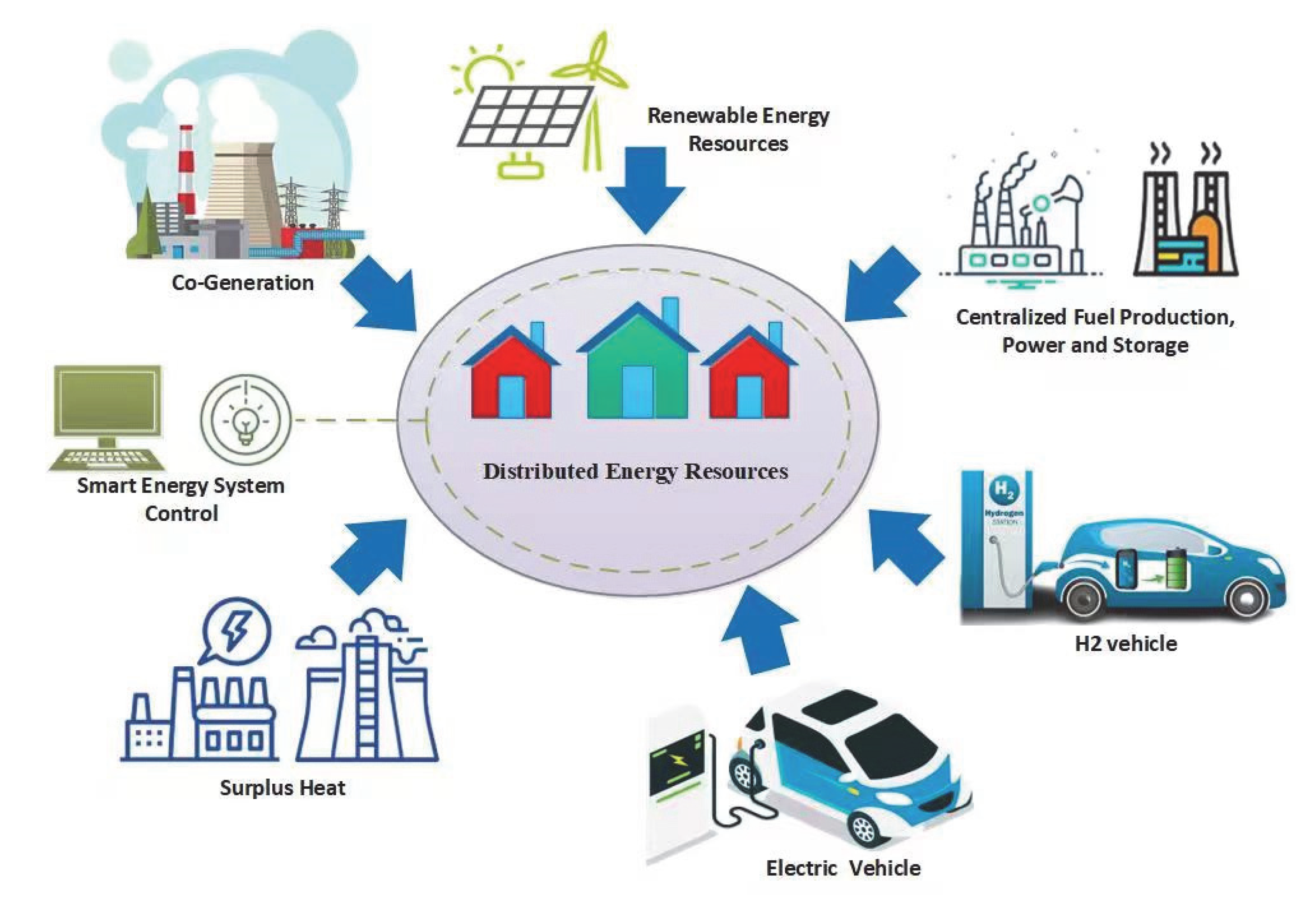
According to Figure 1, the IES encompasses a range of energy flow types, such as cold, heat, electricity, and gas, and its regulation potential is no longer restricted to conventional electrical loads. The power station is comprised of a compressor, expander, gas storage chamber, heat exchange/cooler, heat storage/cooler, and other main components. There is a complex coupling relationship between the internal air mass flow, heat storage and power generation, air pressure, and other variables. Constraints such as pressure change rate constraint, heat exchange power constraint, operating condition and power constraint, and the air storage chamber pressure constraint should be satisfied when scheduling the operation [20].

An IES model includes four energy forms (cold, heat, electricity, and gas), mainly including a gas turbine, an ACA power station, a heat pump, electric refrigerator, absorption refrigerator, wind turbine, gas boiler, integrated energy storage device, and other equipment. Additionally, an IES implements an extensive user-side demand response, directs users to alter their energy consumption mode through signals of energy price changes, indirectly manages the reduction, transfer, and transformation of various energy flows, and enhances the system’s operational flexibility [19]. Therefore, the nature of loads includes fixed loads, transferable loads, and substitutable loads, from the perspectives of the same load’s demand transfer and different load’s energy replacement. The established integrated demand response (IDR) model is:

$$X_L=X_L^f+X_L^p+X_L^r$$

(1)

where XL is the load value after the implementation of the demand response; $X_L^f$ is the fixed load value; $X_L^p$ is the transferable load value; and $X_L^r$ is the alternative load value.

In the day-ahead scheduling process, interruption transfer is not allowed. Therefore, fixed load value is not related to price information. For transferable loads, users can increase or decrease the number of partial loads at the current moment according to the energy price signal, or use the energy storage device to translate and adjust the energy in a certain period. Its price response characteristics can be expressed as follows:

$$X_{L.t}^p=X_{L.t}^{p0}+{\displaystyle \sum _{t\in T_R}{\epsilon }_{t{t}^{’}}^{Lp}}{X}_{L.t}^{p0}({\rho }_{t^{’}}^e-{\rho }_{t^{’}}^{e0})/{\rho }_{t^{’}}^{e0}$$

(2)

where $X_{L.t}^p$ is the transferable load before the implementation of the demand response at time t; ${\epsilon }_{t{t}^{’}}^{Lp}$ is the load price mutual elasticity coefficient at t moment and t′ moment; T_R is the set of time; and ${\rho }_{t^{’}}^{e0}$ and ρ represents t actual load price and base price, respectively.

For alternative loads, users comprehensively compare energy prices (electricity, gas, heating, and cooling prices), which can change with variety, and, combined with their willingness to participate in the demand response of the load value, the price of the properties can be expressed as:

$$P_{L.t}^r=P_{L.t}^{r0}+{\displaystyle \sum _{i\in X}{\lambda }_{}^{ei}}{\epsilon }_t^{ei}{X}_{L.t}^i({\rho }_{t^{’}}^i-{\rho }_{t^{’}}^{i0})/{\rho }_{t^{’}}^{i0}$$

(3)

where $P_{L.t}^{r0}$ and t are the substitutable loads before the implementation of demand response at time t; ${\lambda }_{}^{ei}$ is the conversion efficiency of electrical energy to other energy; ${\epsilon }_t^{ei}$ is the cross elasticity coefficient; X represents the energy flow except electric energy (gas heat and cold energy flow); $X_{L.t}^i$ is the load value of energy flow i at time t; and ${\rho }_{t^{’}}^i$ and ${\rho }_{t^{’}}^{i0}$ represent the actual price and benchmark price, respectively, of the flow i at time t.

The energy purchase scheduling focuses on minimising daily IES operating costs. The operating cost is mainly composed of natural gas purchase cost C_GT, electric energy purchase cost CEM, and energy conversion and storage equipment operation and maintenance cost C_M, represented as:

$$C_{OP}=C_{GT}+C_{EM}+C_M$$

(4)

The purchase cost of natural gas is shown in Equation (5).

$$C_{GT}={\displaystyle \sum _{s\in \Omega }{\pi }_s}{\displaystyle \sum _{t=1}^{24}({\rho }_{s,g}{F}_{s,t}^C\mathsf{\Delta }t)}$$

(5)

where Ω is the set of all possible purchase price scenarios; s is the scene marker variable; ${\pi }_s$ is the probability of the corresponding scenario; ${\rho }_{s,g}$ is the gas purchase price in scenario S; $F_{s,t}^C$ is the purchased gas volume at time t, and $\mathsf{\Delta }t$ refers to unit scheduling time. The purchase cost of electric energy is as follows:

$$C_{EM}={\displaystyle \sum _s{\pi }_s}{\displaystyle \sum _{t=1}^{24}({\rho }_{{}_{s,e}}^C{P}_{s,e}^C\mathsf{\Delta }t)}$$

(6)

where ${\rho }_{{}_{s,e}}^C$ is the power purchase price in scenario s and $P_{s,e}^C$ is the purchased electric quantity in scenario s. The cost of equipment operation and maintenance is shown as:

$$C_M={\displaystyle \sum _{t=1}^{24}(C_{{}_F}^{CHP}{U}_t^{CHP}\mathsf{\Delta }t)}+{\displaystyle \sum _s{\pi }_s}{\displaystyle \sum _{t=1}^{24}\left[c_{CHP}{P}_{s,t}^{CHP}{c}_{GB}{H}_{s,t}^{HP}+c_{CAES}{P}_{s,t}^{CAES}+c_{AC}{C}_{s,t}^{AC}+c_{EC}{C}_{s,t}^{EC}\right]\mathsf{\Delta }t}$$

(7)

where $C_{{}_F}^{CHP}$ is the start-up and shutdown cost of the CHP unit and $U_t^{CHP}$ is the corresponding unit start–stop variable. Since the start–stop status of CHP units cannot be changed with the fluctuation of the energy purchase price within a day after the day-ahead scheduling plan is made, the start–stop variable takes the same value in all scenarios of the energy purchase price. Combined cooling heat and power (CCHP), $c_{CAES}$, $c_{GB}$, $c_{CHP}$, $c_{AC}$, and $c_{EC}$ represent CHP, and the unit maintenance cost of the unit, ACA power station, gas boiler, heat pump, absorption chiller, and electric chiller, respectively; $P_{s,t}^{CHP}$ stands for the electrical power output of CHP unit; $P_{s,t}^{CAES}$ represents the compression/generation power of ACA station; $c_{GB}$ and $H_{s,t}^{HP}$ represent the thermal power output by gas boiler and heat pump, respectively; and $C_{s,t}^{AC}$ and $C_{s,t}^{EC}$ stand for the cooling power output by absorption chiller and electric chiller, respectively.

3. Proposed Method

To deal with the uncertain characteristics of multiple scheduling resources during IES operation, the hybrid shuffled frog-leaping and local search algorithm (HSFL–LS) was created to establish the IES day-ahead optimisation scheduling model when facing multiple uncertainties, and the bat algorithm was used to obtain scenery. The model comprehensively considers the uncertain characteristics of wind power, energy purchase price, and comprehensive demand response. In the worst case of uncertainty of output and comprehensive demand response, the total cost is obtained under multiple purchase price cases.

3.1. Objective Function

The IES day-ahead economic scheduling model established is essentially a robustness optimisation model. Therefore, it can be transformed into a two-stage and three-layer min–min–max model, based on the idea of an engineering game as:

$$Mi{n}_{\psi ,U}(C_1+Mi{n}_{\psi ,M}Ma{x}_{\psi ,L}{C}_2)$$

(8)

$$C_1={\displaystyle \sum _{t=1}^{24}(C_{{}_F}^{CHP}{U}_t^{CHP}\mathsf{\Delta }t)}$$

(9)

$$C_2={\displaystyle \sum _s{\pi }_s{\displaystyle \sum _{t=1}^{24}\left[c_{CHP}{H}_{s,t}^{CHP}+c_{CHP}{P}_{s,t}^{CHP}+c_{GB}{H}_{s,t}^{GB}+c_{HP}{H}_{s,t}^{HP}+c_{AC}{C}_{s,t}^{AC}+c_{EC}{C}_{s,t}^{EC}+{\rho }_{s,g}{F}_{s,t}^C+{\rho }_{{}_{s,e}}^C{P}_{s,t}^C\right]}}\mathsf{\Delta }t$$

(10)

where C₁ and C₂ are start-up and shut-down costs of CHP units in the first stage, and operation costs and purchasing costs in the second stage, while $Ma{x}_{\psi ,L}$ are the upper, middle, and lower decision variables.

3.2. Constraints

In the comprehensive demand response, the cooling and heating load curves have a certain fluctuation range compared with the power subsystem, and the cooling and heating subsystem allows a certain amount of cooling and heat abandonment. The model considers the sufficiency of cold and hot power supply in the worst case in day-ahead scheduling as:

$$H_{s,t}^{HP}+{\eta }_{HAD}{H}_{s,t}^{HAD}+H_{s,t}^{HP}+H_{s,t}^{CAESg}\ge H_{s,t}^L+H_{s,t}^{HAC}+H_{s,t}^{CAESc}$$

(11)

$$C_{s,t}^{AC}+{\eta }_{CAD}{C}_{s,t}^{CAD}+C_{s,t}^{EC}+C_{s,t}^{CAES}\ge C_{s,t}^L+C_{s,t}^{CAC}$$

(12)

where $H_{s,t}^{HAD}$ and $H_{s,t}^{HAC}$ are the heat supply and heat storage power of the heat reservoir, respectively; $H_{s,t}^{CAESg}$ and $H_{s,t}^{CAESc}$ are thermal load power; $C_{s,t}^{CAD}$ and $C_{s,t}^{CAC}$ represent cold storage and cold storage power, respectively; $C_{s,t}^{CAES}$ is the cooling power for the ACA power station; $C_{s,t}^L$ is cooling load, and ${\eta }_{HAD}$ and ${\eta }_{CAD}$ are the heating efficiency and cooling efficiency, respectively.

Heat storage and cold storage systems can be modelled by analogy by establishing the relationship between energy storage capacity, charging and discharging power, and the constraint of starting and ending energy balance.

The capacity constraints of energy storage system can be represented as:

$$S_{s,t}=\frac{(1-\mu )S_{s,t-1}+({\eta }_C{Q}_{s,t}^C-Q_{s,t}^D)\mathsf{\Delta }t}{S_{all}}$$

(13)

$$S_{\min }\ge S_{s,t}\ge S_{\max }$$

(14)

where $S_{s,t}$ is the energy storage device; S_max and S_min are the energy storage device’s maximum and minimum capacity states, respectively; S_all is the total capacity of the energy storage device; μ represents attrition rate; $Q_{s,t}^C$, $Q_{s,t}^D$ are charge/discharge energy work, respectively; and ${\eta }_C$ is charging efficiency rate.

The power constraints of energy storage system are:

$$\begin{array}{l}{\delta }_t^C{Q}_{\min }^C\ge Q_{s,t}^C\ge {\delta }_t^C{Q}_{\max }^C\\ {\delta }_t^D{Q}_{\min }^D\ge Q_{s,t}^D\ge {\delta }_t^D{Q}_{\max }^D\\ {\delta }_t^D+{\delta }_t^C\ge 1,{\delta }_t^D+{\delta }_t^C\in (0,1)\end{array}\}$$

(15)

where $Q_{\min }^C$ and $Q_{\max }^C$ represent the energy storage device’s minimum and maximum charging power, respectively; superscript D represents the corresponding discharge power; and ${\delta }_t^C$ and ${\delta }_t^D$ are the flag variables of charge and discharge energy, respectively.

The operating conditions and power constraints are:

$$\begin{array}{l}{P}_{c\min }^{CAES}{u}_{CAESc,t}\ge P_{s,t}^{CAESc}\ge P_{c\max }^{CAES}{u}_{CAESc,t}\\ P_{g\min }^{CAES}{u}_{CAESg,t}\ge P_{s,t}^{CAESg}\ge P_{g\max }^{CAES}{u}_{CAESg,t}\\ u_{CAESg,t}+u_{CAESc,t}\ge 1\end{array}\}$$

(16)

where $u_{CAESg,t}$ and $u_{CAESc,t}$ are the indicator variables of ACA power stations in power generation and compression conditions, respectively;$P_{c\min }^{CAES}$ and $P_{c\max }^{CAES}$ are the minimum and maximum compressive power of ACA power stations, respectively; and $P_{g\min }^{CAES}$ and $P_{g\max }^{CAES}$ are the minimum and maximum power of ACA power stations, respectively.

The electric power balance constraint is as follows:

$$P_{s.t}^L+P_{s.t}^{DR}+P_{s,t}^{CAESc}+P_{s,t}^{HP}+P_{s,t}^{EC}=P_{s.t}^{RE}+P_{s.t}^{CHP}+P_{s,t}^C+{\eta }_{CAESg}{P}_{s,t}^{CAESg}$$

(17)

where $P_{s.t}^{RE}$ contributes to the wind turbine; $P_{s.t}^{CHP}$ is the output for the CHP unit; $P_{s,t}^C$ is the purchasing power; $P_{s,t}^{CAESg}$ and $P_{s,t}^{CAESc}$ are the generation power and compression power of the ACA station at period T, respectively; $P_{s.t}^{DR}$ is the response of electrical load; $P_{s.t}^L$ is the electronegative charge power rate; ${\eta }_{CAESg}$ is the power generation efficiency of ACA; $P_{s,t}^{HP}$ is the power consumed by the heat pump; and $P_{s,t}^{EC}$ is the power consumed by the electric refrigerator.

3.3. Optimisation Algorithm

In the SFLA–LS algorithm, a group is made up of a population of frogs that are divided into various memeplexes, each of which has its own culture. One of the most effective methods for solving nonlinear optimisation issues is examining patterns. In a local search, this algorithm is a powerful tool. The augmentation of direction vectors such as [0 1], [1 0], [1 0], and [0 1] is the initial stage in using the PS. After establishing the fitness function, the population of P frogs is mostly formed in unintentional instances within the search area, the frog location is the nominated response in this process, and a position vector connects each frog, X_i = [x_i1, x_i2,…, x_iN]. According to their fitness, the frogs are listed in descending order. In this algorithm, the mth frog goes to the mth memeplex, and frog m + 1 returns to the first memeplex. The frog position with the best fitness is represented by X_b, and the frog position with the worst fitness is introduced with X_w. Xg also defines the global best fitness. Following that, a particular technique is performed to improve the fitness of the frog with the lowest fitness level, such as:

$$D_i=Rand\times \left(X_b-X_w\right)$$

(18)

$$X_w^{new}=X_w^{old}+D_i\left(D_{i\min }\le D_i\le D_{i\max }\right)$$

(19)

When a better solution is found, it swaps places with the worst frog. Otherwise, Equations (18) and (19) are solved again; however, X_b is substituted with X_g. Without any enhancement in results, a novel result can be arbitrarily created to interchange that frog.

When the objective function is unable to be observed in a given iteration, an amendment factor is used to reproduce the initial position (0.5). This strategy results in a reduced objective function, and the practice is repeated until the stopping principles are met, as shown in Figure 2. The HSFLA–LS method uses a series of pre-generated discrete examples to describe the uncertainty of energy purchase price. Each case has a set of electricity and gas purchase prices, as well as the case’s chance of occurrence. In one scenario, the IES works as a price receiver, establishing a constraint set for each energy purchase price case in order to solve the scheduling model and retrieve the relevant electricity and natural gas transaction quantities. Based on the energy purchase prices for all cases, and the related amounts of electricity and natural gas, the quote curve for each scheduling period may be determined. This creates the quotation plan that IES offers the energy purchase market before the deadline. This paper uses a heuristic search to find the worst implementation case of uncertainty factors using the HSFLA–LS algorithm with a penalty function constraint.

To solve the established double-loop model, and obtain the robust optimal solution of IES scheduling strategy, the worst impact of uncertainty is considered. The outer loop comprehensively considers the profit and occurrence probability of all cases for IES operators, and minimises the IES expected operating costs by arranging CHP unit start–stop plans. In the inner loop, the IES operators consider multiple possible energy purchase price cases based on the random case method, and realise the safe and economical operation of the system by coordinating the intra-day scheduling resources after the start–stop plan and actual available scenery output and comprehensive demand response of the CHP units are given.

4. Result and Discussion

4.1. Model Parameter Setting

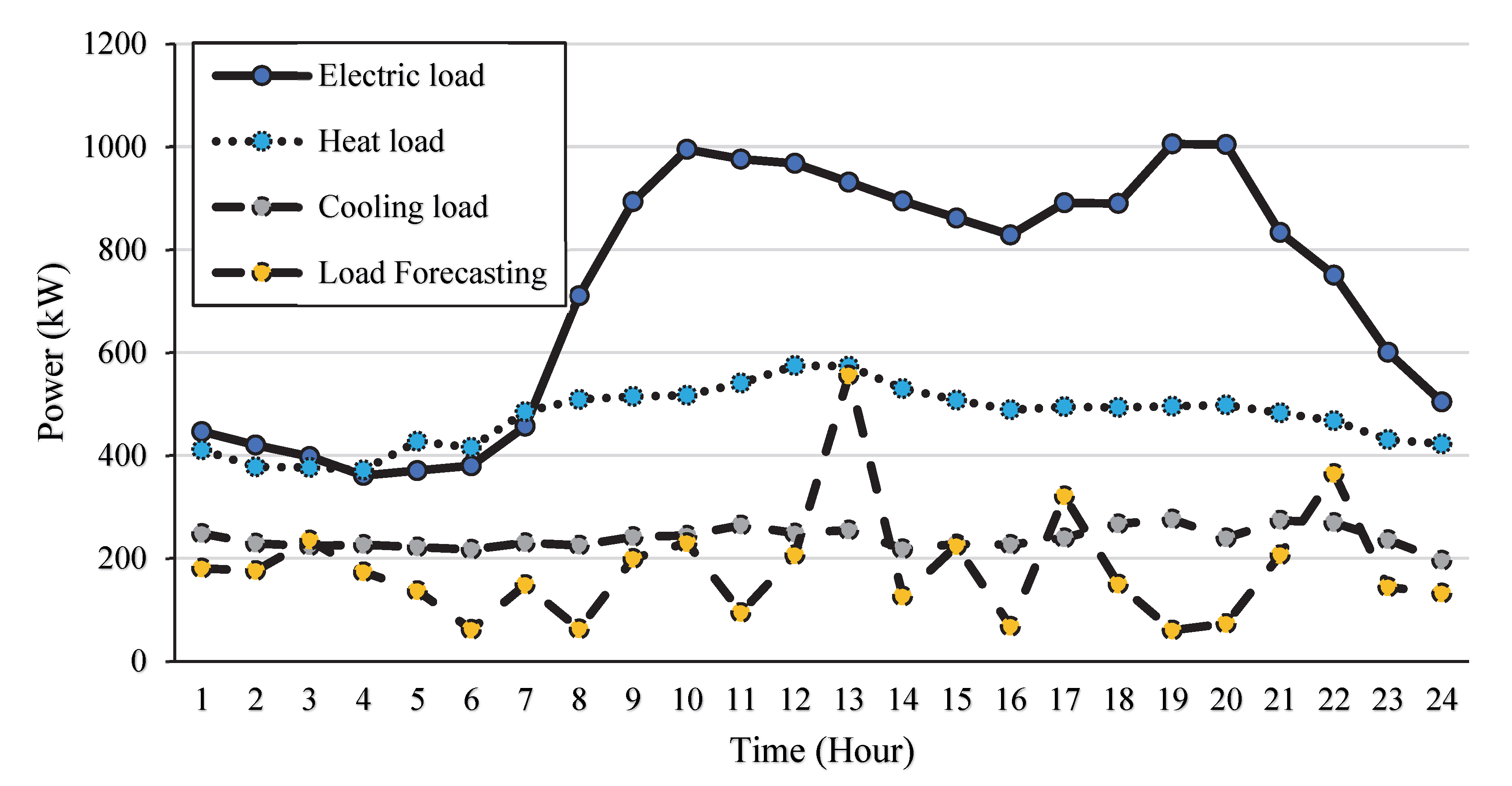
As a simulation example, the actual integrated energy system parameters in a particular area are used. Figure 3 displays the integrated energy system’s power, heat, and cooling load numbers, as well as the available scenic output during the scheduling period. The prediction error of wind output and the uncertainty fluctuation range of comprehensive demand response is 20%.

The electricity purchase market adopts the form of price, in which 01:00–08:00 and 23:00–24:00 are 0.24 USD/(kW·h) in the valley period, 09:00–11:00 and 21 in the normal period. It is 0.57 USD/(kW·h) from 00 to 22:00, and 0.95 USD/(kW·h) in the peak period from 12:00 to 20:00. In this paper, five cases are generated using historical data in which the power purchase price is considered volatile, and the fluctuation range is 40%. The cold, heat, and gas prices are fixed, and are 0.85 USD/(kW·h), 0.35 USD/(kW·h) and 1.87 USD/m³, respectively. The scheduling period T is 24, and the unit time interval is 1 h.

Table 1. ACA scheduling parameters.

Parameter	Values
Rated compression power/kW	100
Rated power/kW	100
Gas storage chamber volume/m3	5.5 × 105
Initial pressure of the gas storage chamber/bar	47.5
Upper pressure of gas storage chamber/bar	55
Lower limit of air storage chamber pressure/bar	40
Unit capacity maintenance cost/(USD/kWh)	0.729

shows the ACA scheduling parameters. Gas turbine parameters, heat/cold storage system parameters, and other equipment parameters are detailed in [26].

4.2. Analysis of Model Optimisation Results

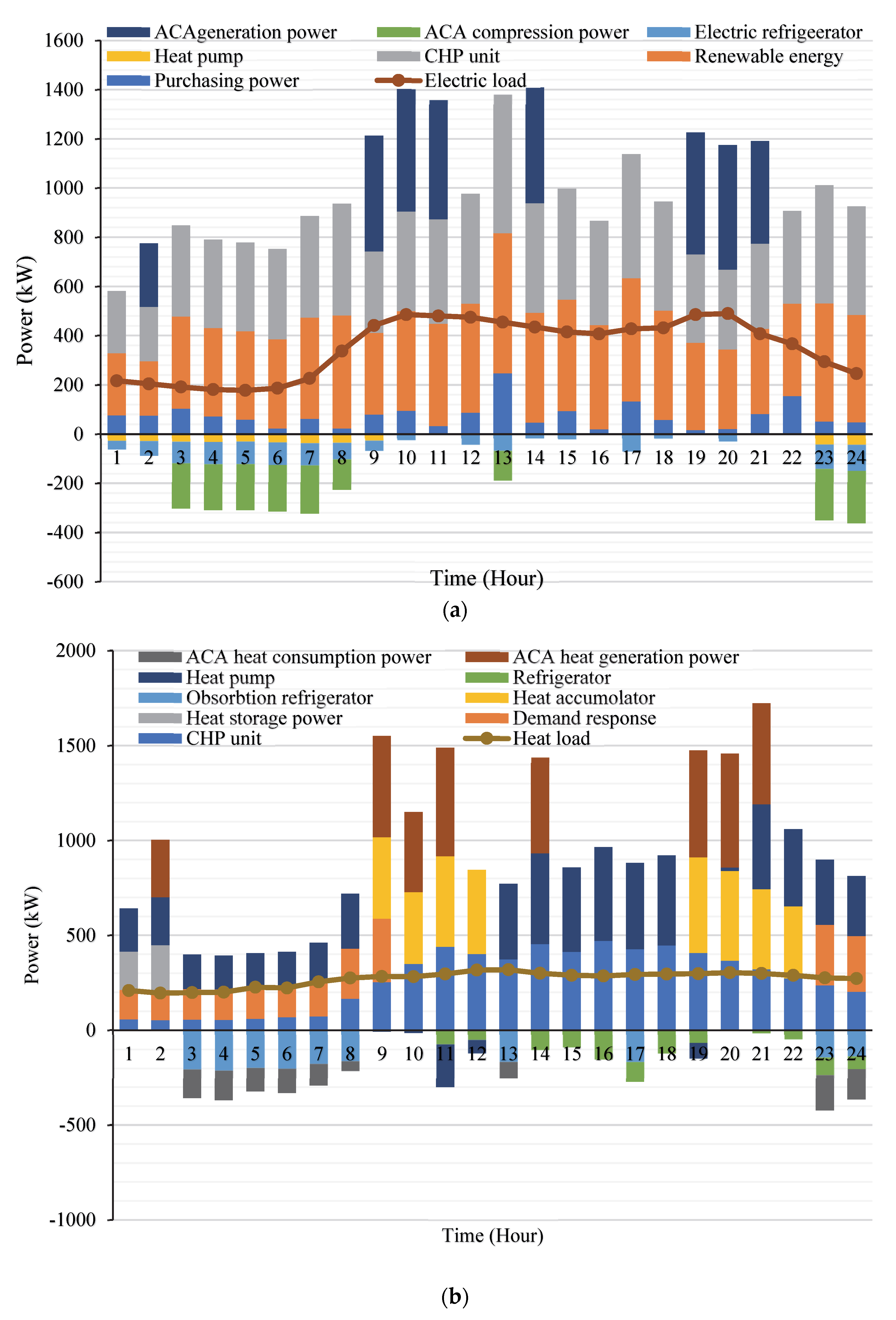
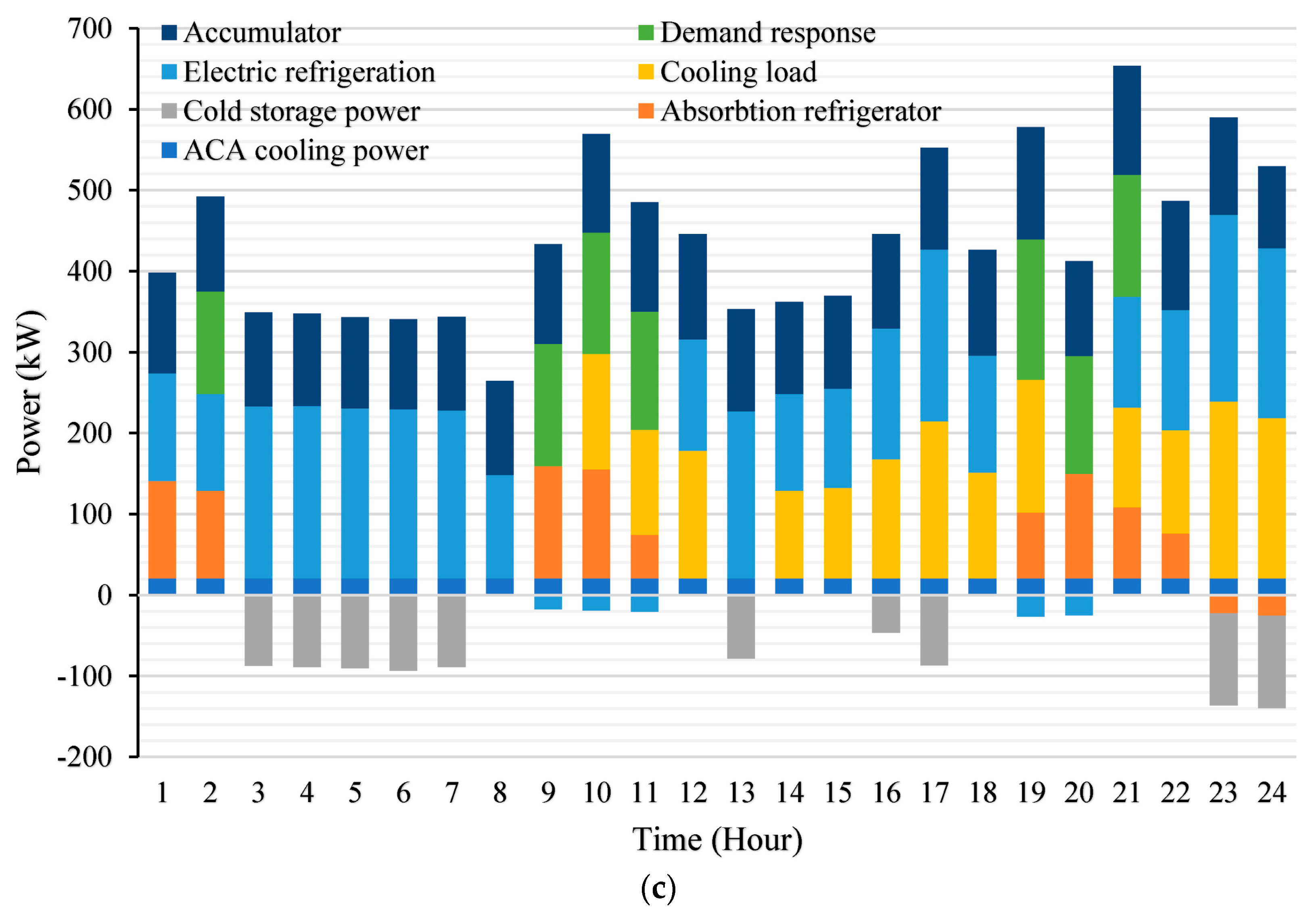
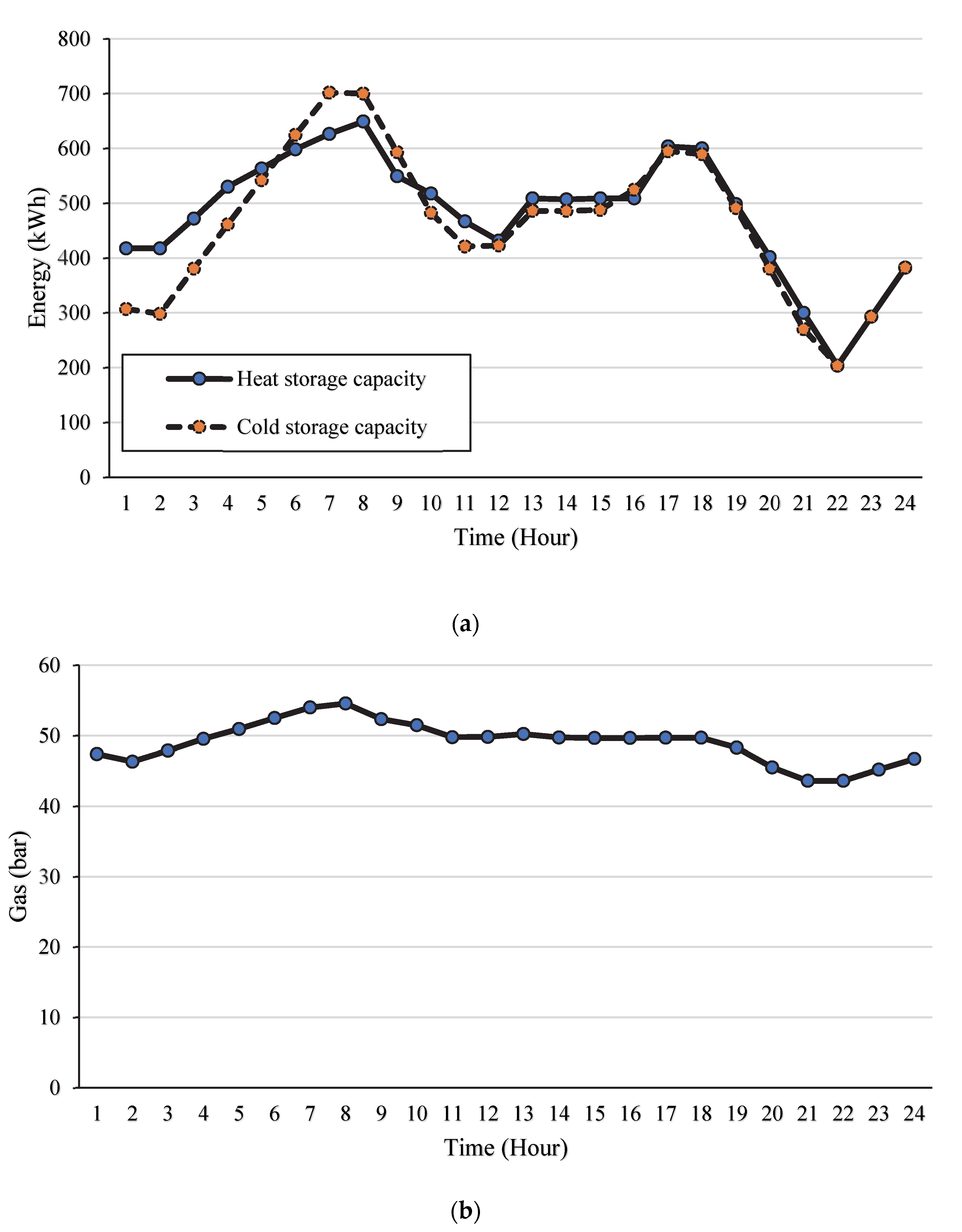
Figure 4 displays the capacity variations of the heat storage/cold storage system, as well as the outcomes of the optimization of the electric, heat, and cold scheduling of the IES. The operating cost is USD 595.68, and the average relaxation power is 308.05 kW.

From Figure 5, the electricity load during 01:00–09:00 and 22:00–24:00 is mainly satisfied by purchasing power and scenery output power. It mainly comprises CHP unit output, ACA plant discharge power and output power meet, and the comprehensive demand response by raising electricity prices to reduce the peak demand. The ACA power station stores part of the surplus electricity under compression conditions, and the air pressure of the gas storage chamber rises. The comprehensive demand response improves users’ willingness to use electricity by reducing prices. From 10:00 to 21:00, a rising system of electric power load buys most of the electricity market in the peak period of electricity price, during the electricity peace time interval at this time, in order to save system costs and power load. Additionally, the ACA power plant’s output curve satisfies the “low storage and high discharge” output characteristic, and offers variable power regulation capabilities.

In the meantime, the features of the CHP-fed power supply can work in harmony with heating and cooling apparatus to maximize the efficiency and adaptability of system operation. As heat pumps and electric refrigerators have great energy conversion efficiency, they can use a relatively minimal quantity of electric energy to satisfy consumers’ heating and cooling needs. Therefore, increasing their output ratios can improve the system’s operation economy when making scheduling plans. In the whole operation cycle, the ACA power station and the integrated energy storage devices can integrate according to the purchase price peak, and can manage the demand response load fluctuations in both energy storage release and load transfer in the increase or decrease in demand. To alleviate renewable energy supply and the area between peak load demand time, the ability of the renewable energy given must be improved, to effectively improve the economic benefits of the integrated energy system operation.

4.3. Influence of Uncertain Factors

We specified the comprehensive, integrated energy system after considering uncertain scheduling policy effectiveness and superiority. According to the source of the uncertainty modelling methods, we set up four cases: the contrast analysis of renewable energy output uncertainty, the integrated demand responding to uncertainty, and the influence of purchase price uncertainty on integrated energy system scheduling results. The specific scene settings are described as follows.

Case 1: The scheduling model is deterministic and does not consider the impact of uncertain factors;

Case 2: In the scheduling model, the stochastic case method is used to model the uncertainty of energy purchase price, and the predicted value of scenery output power and comprehensive demand response is taken;

Case 3: In the scheduling model, a robust optimisation method is used to model the uncertainty of scenery output and comprehensive demand response, and the purchase price is set to a specific scene;

Case 4: In the scheduling model, the robust optimisation method is used to model the uncertainty of scenery and comprehensive demand response, and the random case method is used to model the uncertainty of purchase price.

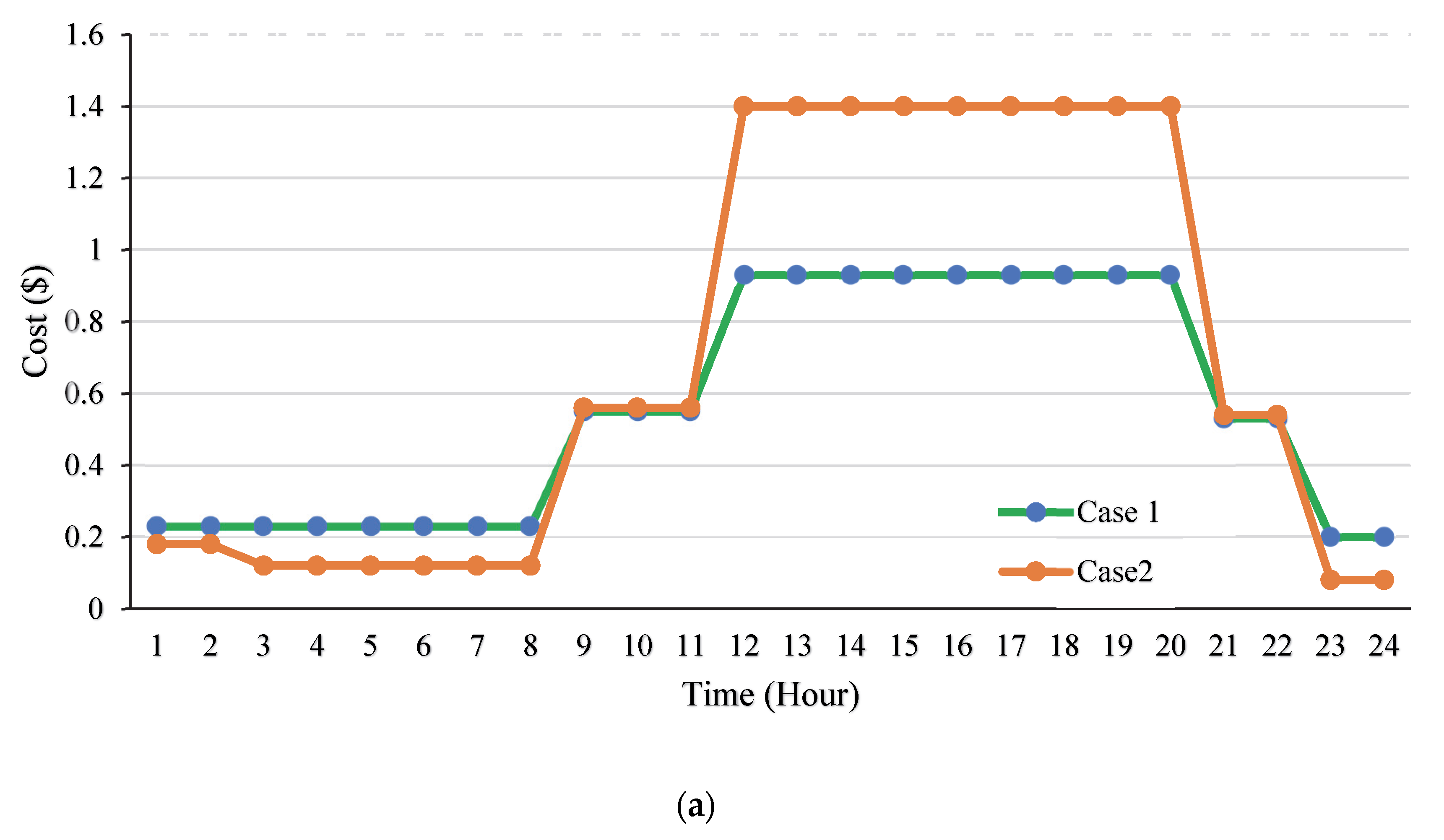
To further illustrate the impact of energy purchase price uncertainty on the economy of model scheduling results, case 2 was selected for analysis, only considering the uncertainty of energy purchase price. The electricity purchase price and purchase quantity of case 1 and case 2 are shown in Figure 6.

The purchase price and quantity of power in examples 1 and 2 varies significantly with case 2’s purchase price fluctuating more wildly than case 1, and its peak–valley difference being bigger. Therefore, IES operating costs choose more electricity during the price valley period to supply electricity load demand, or store it in the ACA power station. The appropriate purchase of IES operating costs reduces the purchase of electricity during the price peak period to meet regional electricity load demand, reducing the electricity purchase price in case 2.

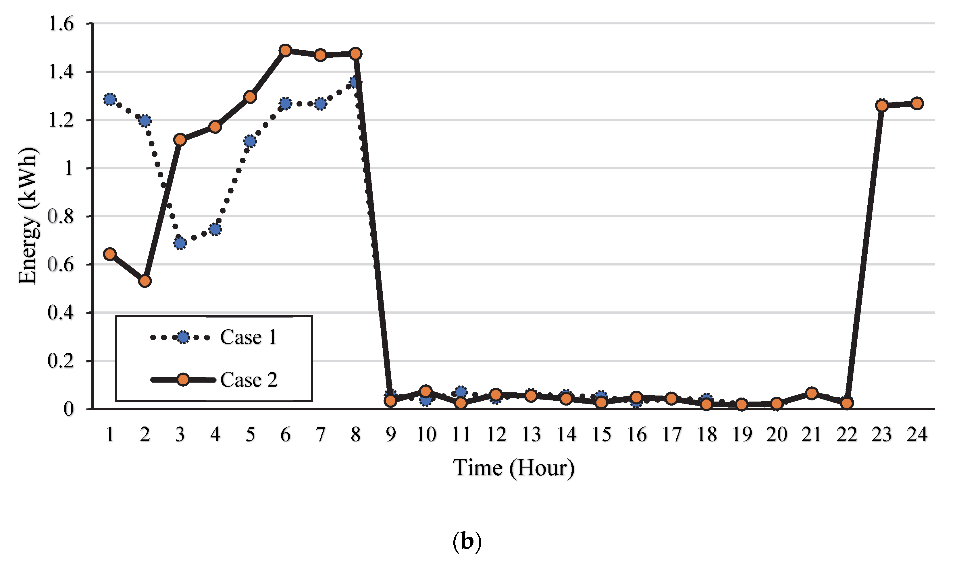
We explored the influence of wind-output uncertainty and comprehensive demand response uncertainty on IES operation economy and safety. In the model, the comprehensive demand response is involved in the positive and negative rotational reserve constraints of electrical loads, and the power balance constraints of hot and cold loads. Its uncertainty directly relates to the operation economy and security of multiple electricity, heat, and cold subsystems. 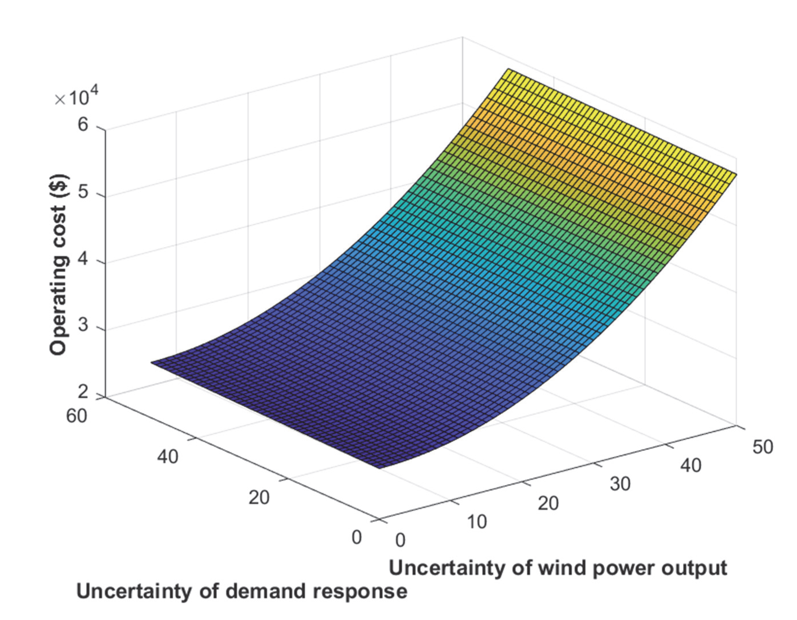Figure 7 and Figure 8 show that with the increase in the value of the uncertain budget set, IES operating cost shows an increasing trend, while the average slack power also decreases. This suggests that although large, unknown budget set values can raise the system’s operating costs, they can also increase the IES’s operational security. IES operators can balance system operation economy and robustness based on the current circumstances, and they may coordinate and optimize economy and robustness through the reasonable value of the allocated uncertain budget. By comparing the scheduling results under different values of ψ_RE and ψ_DR, it can be seen that the change in the comprehensive demand response uncertain budget has a more significant impact on the operation cost and average slack power of IES than the change in the scenic output uncertain budget.

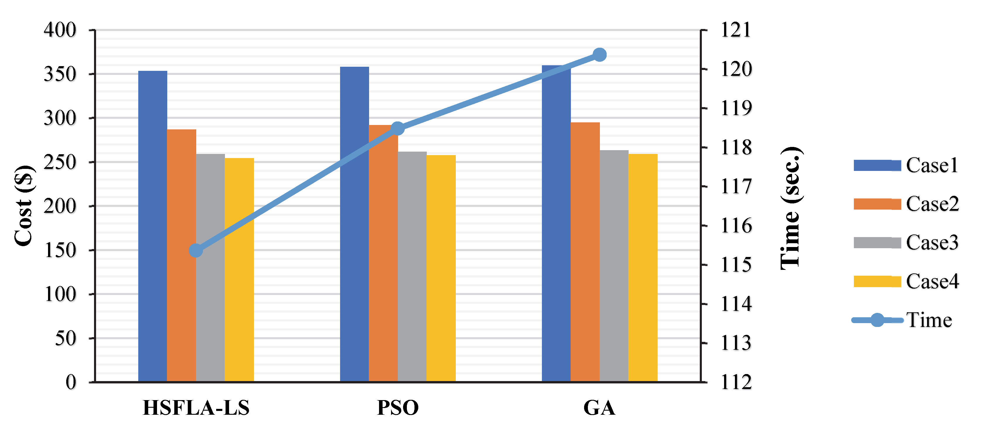
Figure 9 shows the final comparison of the operating costs for the four cases of the various algorithms, and the processing time among various methods. After considering the hybrid SFLA–LS algorithm for different cases, the uncertainty of energy purchase price in case 4 is reduced by USD 14.7 (5.77%), USD 32.6 (12.8%), and USD 89.1 (35%), compared to case 3, case 2, and case 1, respectively. Therefore, it is clear that, after considering scenery output and comprehensive demand response uncertainty, the model’s robustness is improved by sacrificing certain economic benefits. The hybrid SFLA–LS algorithm further optimises the uncertainty of the energy purchase model in case 4, which is reduced by USD 1.63 (0.64%) and USD 3.34 (1.3%), compared to PSO and GA, respectively. In addition, the time for the execution of the SFLA–LS algorithm is reduced by 1.886 s (1.59%), and 3.117 s (2.7%), compared to PSO and GA, respectively. Nonetheless, the hybrid SFLA–LS algorithm dramatically increases the profit cost, enhances the IES’s total cost, and the system can be flexibly adjusted according to the real-time market electricity price and the operating cost.

5. Conclusions

In this paper, an IES is comprehensively studied with multiple uncertain sources such as output uncertainty, energy purchase price uncertainty, and comprehensive demand response uncertainty. The feature identification of uncertain sources, the random scene method, and the robust optimisation method are used to model the uncertain sources, and are optimised based on the proposed HSFLA–LS algorithm. The conclusion can be summarised as follows:

(1)

Considering the unpredictability of the price of energy purchases, IES operators can choose the best energy buy strategy in real-time, based on the particular market price realization scenario, enhancing the system’s operational economy;

(2)

The economic scheduling model considering multiple uncertainties proposed in this paper can further enhance the economy and security of system operation, in accordance with the characteristics of uncertain sources when comparing the HSFLA–LS model with the deterministic scheduling model and the model considering only a single uncertainty;

(3)

The best way to operate the IES and identify the best output for the ACA device is to use a hybrid SFLA–LS algorithm. The result that has the biggest effect on the system’s security and overall economy is the modification to apply to the comprehensive demand response uncertainty budget.