Article

Enhanced Agriculture Insurance with Climate Forecast

1
Accounting Department of Business School, Hunan International Economics University, Changsha 410205, China
2
Department of Applied Economics, School of Economics and Management, Yango University, Fuzhou 350015, China
3
Department of Insurance and Finance, National Taichung University, Taichung 403336, Taiwan
4
Department of Finance, College of Finance, Feng Chia University, Taichung 407102, Taiwan
5
Gordon S. Lang School of Business and Economics, University of Guelph, Guelph, ON N1G 2W1, Canada
*
Author to whom correspondence should be addressed.
Sustainability 2022, 14(17), 10617; https://doi.org/10.3390/su141710617
Submission received: 20 July 2022 / Revised: 20 August 2022 / Accepted: 22 August 2022 / Published: 25 August 2022
(This article belongs to the Special Issue Risk Management and Actuarial Science for Sustainable Agribusiness)

Abstract

:
This paper presents a model to study how climate forecasts and the agricultural production function affect the effectiveness of government policies (disaster bailouts and agricultural income tax) and agricultural insurance (both compulsory and voluntary). In the base model with a neoclassical production function, we find that these programs could increase farmers’ expected profit and reduce its volatility. Furthermore, credible climate forecasts enable farmers, insurance companies, and governments to make more informed cultivate and insurance decisions, and therefore increase the benefit of these insurance programs to farmers. The results suggest that climate forecasts, combined with agriculture policies and insurance, can play an important role in securing farmers’ profits and providing climate risk management guidance for agriculture production.

1. Introduction

Farmers endure various market and production risks, and sometimes also suffer extreme climate conditions, such as droughts, floods, or storms. Such risks may be diversified in insurance markets and credit markets. According to the Centre for Science and Environment (2016), more than 100 countries have agricultural (crop and livestock) insurance markets. Since the late 1990s, government subsidies to agricultural producers in emerging markets have been disappointing or disastrous [1]. Agricultural insurance products (combined with other risk financing instruments such as savings and credit) can enhance agricultural profitability in developing economies. Ref. [2] showed that the positive correlation between crop productivity and insurance takeup is stronger for group-performance-based policies than individual-performance-based policies. The World Bank and donors support insurance pools as well as index-based insurance. The agricultural sector has become more profitable and commercial than it once was.
Agricultural insurances have various covers, which contain three types of crop production insurance: individual yield, area yield, and climate index insurance. These crop insurance products insure farmers against losses caused by climate-related disasters. Conventional individual-yield crop insurance makes an indemnity payment when a farm or commodity incurs a yield loss. Conventional individual-yield crop insurance includes products such as hail insurance, which is offered in most organizations for Economic Co-operation and Development countries. Area-yield crop insurance provides indemnities and premiums based on the aggregate yield of a geographical area. Such insurance products already exist in the USA, India, and Sweden. In the USA, a typical group risk plan employs county yields to trigger a payment, and its coverage reaches up to 90% of the county yield. Climate index insurance provides an indemnity based on the values provided by a climate index that serves as a proxy for losses. Among climate index insurance products, rainfall insurance contracts may be technically more feasible than other indices for most countries because long data series from regional climate stations are available. Climate insurance is popular because it has low administration costs and no moral hazards.
Regarding insurance participation, there are three forms of insurance: voluntary insurance, compulsory insurance, and government bailouts. To protect agriculture industry, governments may require farmers to buy compulsory insurance to offer basic coverage of loss resulting from weather-related disasters. Moreover, government bailouts are often used to provide extra coverage in addition to compulsory insurance. Finally, in addition to compulsory insurance and government bailouts, farmers may purchase voluntary insurance to protect their individual different incomes. Theoretically speaking, each insurance form could take any of the three types of coverage introduced above. For example, a compulsory insurance program could insure individual yield or area yield, or have payments linked to a climate index. Related literature on agriculture insurance only discuss one insurance type under climate forecasting [2,3]. In this paper, we will investigate the potential of all the three forms of insurance on insuring agriculture production risk and the impact of climate forecasts on the efficacy of these insurances.
This study develops a framework for analyzing the effect of climate forecasts and the agricultural production function on the effectiveness of both government policy (disaster bailouts and agricultural income tax) and agricultural insurance (both compulsory and voluntary). Although [3] discussed insurance, climate forecasts, and production, they do not discuss the efficiency of government policy and agricultural insurance at different stages of production function under climate forecast. Our study incorporates different insurance types, different government policies and different production stages into the two types of climate forecast model. The proposed concepts for this framework and the findings in this paper are new to the literature. This study makes four major contributions. First, if agricultural production enters the concave stage, voluntary agricultural insurance provides farmers with long-term profits, and compulsory agricultural insurance increases farmers’ overall profits and reduces the volatility of their profits. Second, government agricultural bailouts and income tax may benefit farmers in the long term because of the climate cycle. Third, effective climate forecasts increase the expected value and reduce the volatility of agricultural production if farmers make informed cultivate decisions, i.e., if they only cultivate when climate forecasts are favorable to agriculture production. Finally, if governments make agricultural policies and farmers purchase agriculture insurance with special coverage after climate forecasts have been issued, effective climate forecasts promote the efficacy of both voluntary agriculture insurance and government policy (fewer bailouts and lower taxes). In summary, these results suggest that climate forecasts, agricultural policies and agricultural insurance can have a positive effect on farmers’ profits and provide guidance for farmers conducting climate risk management.
The remainder of this paper is organized as follows. Section 2 provides a literature review of climate forecasts and their impact on agriculture production. Section 3 introduces the base model, agriculture insurance, and the government bailout program. Section 4 discusses the impact of climate forecasts on these insurance programs. Section 5 concludes. Proofs are collected in the Appendix A, Appendix B, Appendix C and Appendix D.

2. Literature Review

The frequency and intensity of climate-related disasters have increased since 1900 (data from the Emergency Events Database, EM-DAT), and then the insured losses increase and vary violently since 1970 (data from sigma from Swiss Re.) as shown in Figure 1. Such climate-related disasters have endangered agriculture worldwide. Millions of farmers face tragic crop or livestock failures. According to the Food and Agriculture Organization of the United Nations, analysis of 78 post-disaster assessments from 2003 to 2013 reveals that agriculture absorbed 25% of the total impact of climate-related disasters in developing countries. Agriculture is vital for supporting the livelihoods of the majority of poor people, who are vulnerable to climate change. According to the World Bank, an additional 122 million people will live in extreme poverty by 2030. Thus, how to manage climate risk in agriculture is a grave concern.
According to the AR6 (Sixth Assessment Report) of the IPCC (Intergovernmental Panel on Climate Change), the near-linear relationship between cumulative CO2 emissions and maximum global surface temperature increase implies that climate change mitigation is to reduce or prevent emissions of greenhouse gases. Ref. [4] review the main strategies for climate change abatement such as conventional mitigation, negative emissions, and radiative forcing geoengineering. An emergent negative emission technology is used to offset additional emissions from sectors where greenhouse gas emissions are difficult or impossible to decrease [5]. Ref. [6] analyzed microalgae’s massive cultivation for CO2 biofixation for negative emissions. However, a 1.5 °C increase is very likely (in the AR6) in the 20-year globally averaged surface air temperature, relative to the average over the period 1850–1900. Therefore, the sustainability of the crop industry depends on adaptation to climate change [7]. There are two climate risk management strategies for the agriculture industry: risk minimization (ex ante) and loss management (ex post) [8]. Ex ante strategies include crop diversification, intercropping, low fertilizer application, poor-quality seeds, and land-sharing cropping. Ex post strategies include liquidation of assets (particularly livestock), family mutual aid networks, self-insuring behavior (savings and credit reserves), off-farm employment, and migratory labor. Although numerous risk management options exist, most are likely to fail during extreme climate events. Because climate risks are covariate, losses become correlated across farmers and may cover large geographical areas. Farmers in the same area all suffer heavy losses whichever ex ante strategies they employ and lose the ability of mutual aid and restructuring. Thus, covariate risk (often called systemic risk) severely limits the efficiency of conventional and informal risk management strategies. Studies have proposed some solutions for improving these two categories of strategies.
Effective climate forecasts improve ex ante risk minimization because farmers can reduce input sources and risk exposure in advance [3]. The feasibility of time diversification contributes to ex post loss management [9]. Seasonal climates are predictable in many world regions [10]. For example, the El Niño Southern Oscillation (ENSO) is linked to variation in seasonal precipitation [11]. ENSO affects yields and production practices. Climate satellites can continuously monitor climate change on Earth. El Niño events historically seem to have occurred at irregular intervals from 2 to 7 years, usually lasting for 1 or 2 years over at least the last 300 years. This cyclic characteristic improves climate-related risk management. Meteorological departments in developed countries offer farmers regular climate forecasts. Governments and farmers can act to reduce loss in advance although some agricultural infrastructure and land cannot avoid damage from extreme climates. Whether ex ante strategies are efficient depends on the accuracy of climate forecasts. Studies on agricultural and climate science contribute to climate forecasts that inform production decisions [12,13]; Rowhanji, 2011. However, most researchers focus on risk management in agriculture under climate change [14,15]; Kuosmanen, 2015. Few studies have investigated the impact of climate forecasts on agricultural insurance and government agricultural policies on tax and bailouts. Ref. [8] showed that the existence of the climate cycle helps governments’ bailout funds achieve a long-term fiscal balance. Ref. [3] discussed insurance, climate forecasts, and production. This paper presents the effects of climate forecasts on compulsory or voluntary agricultural insurance, government bailouts, and tax. The findings provide governments and farmers with valuable insights on how to base policy and decisions.

3. Preliminaries and the Base Model

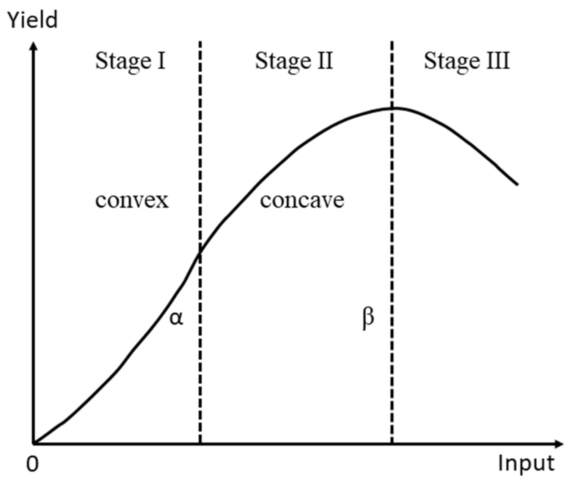
A neoclassical production function in agriculture is illustrated in Figure 2 [16]. This function has been widely used for describing the relationships between input (e.g., seeding, weeding, and application of fertilizers, irrigation, and pesticides) and output (e.g., drying, processing, and preservation) [17]. In the first stage (Stage I), the curve is convex, which means that the rate of marginal product is positive and increasing. That is, as the input increases, so do the productivity and the marginal product, i.e., the productivity of the incremental unit of the input. In the second stage (Stage II), the curve is concave, which means that the rate of marginal product is negative. A maximum marginal product exists at a special level of the input. The inflection point is denoted by α. At that point, the marginal product is at its greatest. After point α, productivity still increases, and the marginal product is also positive but declines. At stage III, productivity reaches its maximum. The marginal product is zero at point β and becomes negative thereafter. Therefore, it is not profitable for farmers to cultivate when the input exceeds this point. Few scholarly articles have discussed the efficiency of agricultural insurance at different stages of this production function. This study develops a simple model to show that purchasing agricultural insurance is not worthwhile if the production function is convex.
Consider competitive farmers producing a single crop with yield y(θ, w) based on the production inputs θ and the climate condition w. The production inputs θ include all costs of seeds, fertilizers, and farming technology. The climate condition w could be either a good climate w = g with historical probability wg or a bad climate w = b with historical probability 1 − wg. Farmers only cultivate if they expect a positive profit in the long term, according to this historical probability. The yield y(θ, g) under good climates is larger than the yield y(θ, b) under bad climates. The expected production at the end of this year is
E [ y ( θ , w ) this   year ] = w g y ( θ , g ) + ( 1 w g ) y ( θ , b )
and the variance of production at the end of this year is
V a r [ y ( θ , w ) this   year ] = w g ( 1 w g ) ( y ( θ , g ) π ( θ , b ) ) 2
We assume that the yield y(θ, w) has the output price p and the input cost c per unit. The profit function for farmers is given by
π ( θ , w ) = p y ( θ , w ) c θ
Because the profit π(θ, w) is a linear function of y(θ, w), it becomes a concave (convex) function if the yield y(θ, w) is a concave (convex) function. The expected profit of this year is determined using the following equation:
E [ π ( θ , w ) this   year ] = w g π ( θ , g ) + ( 1 w g ) π ( θ , b )
and the variance of profit at the end of this year is
V a r [ π ( θ , w ) this   year ] = w g ( 1 w g ) ( π ( θ , g ) π ( θ , b ) ) 2
As shown in the final term of the above equation, the variance is at its maximum value at wg = 0.5.

3.1. Climate Forecasts

This section illustrates how climate forecasts efficiently benefit farmers (detailed proof is given in Appendix A). Consider farmers’ decisions to cultivate if the climate forecast is favorable but do nothing if the climate forecast is bad. Suppose that as climate technology advances, the climate forecast outperforms historical experience. We call it an effective climate forecast. With a good climate forecast, the probability of good climate occurring is wg|g, which is larger than wg but less than 1. The probability of a bad climate becomes 1 − wg|g, which is less than 1 − wg. Effective climate forecasts can raise the expected production because the loss probability decreases (i.e., farmers cultivate less frequently in bad years). Compared with Equation (1), the expectation becomes larger as in Equation (6):
E [ y ( θ , w g g ) this   year ] = w g g y ( θ , g ) + ( 1 w g g ) y ( θ , b ) > E [ y ( θ , w ) this   year ] .
Thus, progress in climate forecast technology increases farmers’ production. Moreover, effective climate forecasts can reduce variance in production. Compared with Equation (2), variance of production declines as in Equation (7).
V a r [ y ( θ , w g ) this   year ] = w g g ( 1 w g g ) ( y ( θ , g ) y ( θ , b ) ) 2 < V a r [ y ( θ , w ) this   year ]
This means that effective climate forecasts contribute to farmers’ profits by helping farmers make efficient production decisions.
From the analysis above, we see that an efficient forecast helps farmers perform ex ante risk management risk by reducing input sources. The benefit resulting from climate forecasts continues for a long time. However, developing reliable forecasting skills requires substantial funding to be invested in technological research and development. Only governments can bear such substantial capital expenditures, which are beyond the means of individuals and insurers. Furthermore, even if climate forecasts are always correct, a sizeable climate event still damages agricultural infrastructure, land, or production tools. Additionally, farmers require funding to restore their productive capacity after such disasters. Such funds may come from agricultural insurance or government bailouts, which we will discuss in the following sections.

3.2. Agricultural Insurance

This section investigates the impact of agricultural insurance on agricultural production. Appendix B provides detailed proofs for all assertions in this section. Agricultural insurance in this study is assumed to be actuarially fair. For convenience, we assume that insurance premium rate τ or claim I is paid at the end of the insured year. Farmers may purchase voluntary agricultural insurance to reduce individual contingent loss. Moreover, governments may implement compulsory agricultural insurance to offer all farmers basic coverages. Under which stage of production voluntary or compulsory insurance are most efficient will be analyzed in the following discussion.
In this analysis, we assume the historical data on climate change reveal one bad year per k years. That is, the occurrence probability of a bad year is 1 − wg = 1/k. Paying insurance premiums reduces the input source in good years, but the insurance claim increases the input source after the bad year. When agricultural production remains at the concave stage, Equation (8) shows that the increment of production at the end of k th year (due to the claim used as the input source at the beginning of k th year) exceeds the sum of decrement in sequential k–1 good years (due to the input source used as the insurance premium):
y ( v + k a , w ) y ( v , w ) > k [ y ( u , w ) y ( u a , w ) ]
where a, u, and v represent the insurance premium, input in good years, and input after bad years, respectively. We see that agricultural insurance is efficient in the concave stage because the total production of insured farmers at the end of k years exceeds that of farmers without agricultural insurance. On the contrary, if agricultural production stays at the convex stage, the production decreased by the premium payments is larger than the production increased by the insurance claim. Therefore, the agricultural insurance is inefficient.

3.2.1. Voluntary Agricultural Insurance

If farmers purchase voluntary agricultural insurance at the beginning of this year, they may pay the premium τ (in a good year) or receive the claim (1 − τ)I (in a bad year) at the end of this year. The profit function with agricultural insurance is denoted by π(θ, w, I), which equals π(θ, g) − τI with probability wg or π(θ, b) − (1 − τ)I with probability 1 − wg. When the insurance is actuarially fair, the expected profit with insurance at the end of this year is equals to that without:
E [ π ( θ , w , I ) this   year ] = w g ( π ( θ , g ) τ I ) + ( 1 w g ) ( π ( θ , b ) + ( 1 τ ) I ) = E [ π ( θ , w ) ]
However, the expected profit with insurance at the end of next year is larger than that without. The reason is that the profit function is also concave if the production function enters the concave stage. Voluntary agricultural insurance thus benefits farmers as shown in Equation (10).
E [ π ( θ , w , I ) next   year ] = ( 1 w g ) π [ y ( v + ( 1 τ ) I ) ] + w g π [ y ( u τ I ) ] > E [ π ( θ , w ) next   year ]

3.2.2. Variance of Profit with Agricultural Insurance

Agricultural insurance also conventionally reduces the variability of the subject matter insured. That is, the payment of an insurance premium to insurers reduces the input source in good years, but the indemnity payment from insurers increases the input source after bad years when farmers suffer loss from weather-related disasters. The decrement of agricultural production difference thus leads to reduced variability in farmers’ incomes. The result is shown in Equation (11).
V a r [ π ( θ , w , I ) this   year ] < V a r [ π ( θ , w ) this   year ] = w g [ π ( θ , g ) τ I E [ π ( θ , w , I ) ] ] 2 + ( 1 w g ) [ π ( θ , b ) + ( 1 τ ) I E [ π ( θ , w , I ) ] ] 2

3.2.3. Compulsory Agricultural Insurance

Some countries required farmers to purchase agricultural insurance to reduce government bailout payments to farmers after disasters. We assume that such insurance products have a uniform coverage I. Since compulsory agriculture insurance applies to all farmers in the country, we consider the aggregate profit of the farmers instead of the single farmer’s profit. The sum of farmers’ profits is expressed by the integral function
Π ( θ , w , I ) = π ( θ , w , I ) d θ
If the profit functions π ( θ , w , I ) in Equations (9) and (10) are replaced with the total profit function Π ( θ , w , I ) , we can obtain Equations (13) and (14) via the same derivation process as for the voluntary agricultural insurance if the total profit function Π ( θ , w , I ) is concave due to the concave stage of total production y ( θ , w , I ) d θ . Again, due to the actuarially fair price of the insurance, the expected profit with insurance at the end of this year is the same as that without:
E [ Π ( θ , w ) this   year ] = E [ Π ( θ , w , I ) this   year ]
However, it will be more than that without at the end of next year.
E [ Π ( θ , w ) this   year ] < E [ Π ( θ , w , I ) this   year ]
Finally, the variance in total profit with compulsory insurance is smaller than the variance without. The derivation process is the same as the one for the voluntary agricultural insurance if we replace the profit function with the total profit function. We obtain the inequality:
V a r [ Π ( θ , w , I ) ] = w g ( 1 w g ) [ [ π ( θ , g ) τ I ] d θ [ π ( θ , b ) + ( 1 τ ) I ] d θ ] 2 < w g ( 1 w g ) [ π ( θ , g ) d θ π ( θ , b ) d θ ] 2 = V a r [ Π ( θ , w ) ] .
Therefore, agricultural compulsory insurance not only increases the expected total profit but also reduces its volatility.

3.3. Government Bailouts and Tax

This section discusses the impact of government policy regarding agricultural bailouts and taxes on the expectation and the volatility of the total profit. The detailed proof for the assertions made in this section is provided in Appendix C.
Consider a case in which the government establishes an agricultural policy whereby farmers are taxed during good years and are bailed out after a bad climate event. The budget constraints require that tax income equals the bailout payments. The tax is calculated by the tax rate q multiplied by the profit with exemption e.
This paper discusses two criteria for bailouts. The first bailout method is to reduce farmers’ costs. The bailout payment is calculated by multiplying the bailout rate s by the inputs θ. The expected bailout is the following integral function:
S = ( 1 w g ) s θ d θ
The following equality between tax income and bailout payments should be satisfied to meet the fiscal requirement of the government:
w g q max ( π ( θ , g ) e ,   0 ) d θ = ( 1 w g ) s θ d θ
Therefore, the relationship between the bailout rate (s) and tax rate (q) is expressed by
q = ( 1 w g ) Π ( θ ) w g Π ( θ , g , e ) s
where Π ( θ , g , e ) = max ( π ( θ , g ) e ,   0 ) d θ and Π ( θ ) = θ d θ .
The total profit for farmers with tax and bailout is expressed as follows:
Π q , s ( θ , w ) = ( π ( θ , g ) q max ( π ( θ , g ) e ,   0 ) ) d θ i f   good   years ( π ( θ , b ) + s θ ) d θ i f   bad   years
The expected total profit with tax and bailout is then given by
E [ Π q , s ( θ , w ) ] = ( w g ( π ( θ , g ) q max ( π ( θ , g ) e ,   0 ) ) + ( 1 w g ) ( π ( θ , b ) + s θ ) d θ = Π ( θ , w )
Although the expected profit remains the same, governments may bail farmers out after bad years, and subsequently, charge income tax when agricultural production enters the concave stage to balance their budget. Such agricultural policies can benefit farmers. The reasons are similar to those in the Agricultural Insurance section, i.e., the bailout is used as an input for higher marginal production after bad years. Income tax is charged on the lower marginal production in good years. Consequently, at the end of the subsequent year, the expected total profit with agricultural bailout and tax is larger than the expected total profit without them. Compared with total profit without agricultural bailout and tax, agricultural bailout and tax can also decrease the volatility of total profit. This means that such policies can improve the redistribution of farmers’ profits.
V a r [ Π q , s ( θ , w ) ] = w g [ π ( θ , g ) q max ( π ( θ , g ) e ,   0 ) d θ E [ Π q , s ( θ , w ) ] ] 2 < V a r [ Π ( θ , w ) ]
The second bailout method is to reduce farmers’ losses. The bailout payment is based on the losses, the negative π(θ, b) over the deductible d. The expected bailout is the following integral function:
S = max ( π ( θ , b ) d ,   0 ) d θ
The following equation should be satisfied to meet the fiscal balance requirement:
w g q max ( π ( θ , g ) e ,   0 ) d θ = ( 1 w g ) max ( π ( θ , b ) d ,   0 ) d θ
The relationship between the bailout rate and the tax rate is expressed by
q = ( 1 w g ) Π ( θ , b , d ) w g Π ( θ , g , e )
where Π ( θ , b , d ) = min ( π ( θ , b ) + d ,   0 ) d θ . The total profit for farmers with tax and bailout is then given by
Π q , s ( θ , w ) = π ( θ , g ) q max ( π ( θ , g ) e ,   0 ) d θ i f   good   years π ( θ , b ) min ( π ( θ , b ) + d ,   0 ) d θ i f   bad   years
Similarly, we obtain the same results as the first bailout method.
Similar to the case of agriculture insurance, efficient forecasting may reduce government bailout payments and thus reduce the tax charged to farmers. As climate forecasts become more efficient, farmers are more likely to make correct production decisions. As a result, the chances of incurring a loss decrease and therefore governments pay less in bailouts in the long term. As bailouts decrease, the income tax rate is adjusted downward. Therefore, it holds that
E [ Π ( θ , w )   next   year ] < E [ Π q , s ( θ , w )   next   year ]
The following derivation process shows that the variance of the total profit with agricultural bailout and tax is lower than that without.
V a r [ Π q , s ( θ , w ) ] = w g [ ( 1 w g ) [ Π ( θ , g ) Π ( θ , b ) ] q Π ( θ , g ) ] 2 + ( 1 w g ) [ w g ( Π ( θ , g ) Π ( θ , b ) ) s θ d θ ] 2 < w g [ ( 1 w g ) ( Π ( θ , g ) Π ( θ , b ) ) ] 2 + ( 1 w g ) [ w g ( Π ( θ , g ) Π ( θ , b ) ) ] 2 = w g ( 1 w g ) [ Π ( θ , g ) Π ( θ , b ) ] 2 = V a r [ Π ( θ , w ) ]
Therefore, the analysis above shows that agricultural bailout and tax can be used to increase farmers’ aggregate profit over the long-term by smoothing their production between good and bad years.

4. Agricultural Insurance and Policy after the Climate Forecast

In the last section, we have discussed the impact of agriculture insurance and government bailout programs on farmers’ profit. This section shows that the benefits of these programs can be further improved with the help of effective climate forecasts. Appendix D provides detailed discussions of the results made in this section.
First of all, let us consider agriculture insurance. When insurers and farmers make insurance and agricultural decisions, they would often rely on the climate forecast for the subsequent year. If the climate forecast is favorable, farmers would cultivate and purchase voluntary insurance against unexpected disasters. When climate forecasts come into play, the insurance premium is fairly adjusted from τ to τb|g to reflect the forecast-adjusted probability of the realization of bad climate conditions, wb|g = 1 − wg|g. That is to say, τb|g = 1wg|g < τ = 1 − wg. The insurance coverage is assumed to be I = π(θ, g) − π(θ, b). Farmers do not cultivate if the climate forecast is bad. In this case, they lose the chance of obtaining profits if the climate turns out to be good conditional on the unfavorable forecasts.
The following equations show that the expected profits with a forecast are larger than those without a forecast (in Equation (28)) and that the variance in profit for insured farmers with a forecast is less than insured farmers without a forecast (in Equation (29)). This means that effective climate forecasts can increase the benefits of agricultural insurance for farmers.
E [ π ( θ , w , I g ) ] = ( 1 w g g ) ( π ( θ , g ) + ( 1 τ b g ) I ) + w g g ( π ( θ , b ) τ b g I ) > E [ π ( θ , w , I ) ]
V a r [ π ( θ , w , I g ) ] = w g g 2 ( 1 w g g ) 2 ( π ( θ , g ) π ( θ , b ) ) 2 < V a r [ π ( θ , w , I ) ] .
When the first bailout method is used, the tax rate is obtained by a similar derivation in Equation (18). The tax rate decreases as the probability wg|g increases when the bailout rate is fixed as follows:
q g = ( 1 w g g ) Π ( θ ) w g g Π ( θ , g ) s < q
When the second bailout method is used, the tax rate is obtained by a similar derivation in Equation (24). The tax rate decreases as the probability wg|g increases when the bailout rate is fixed as follows:
  q g = ( 1 w g g ) Π ( θ , b ) w g g Π ( θ , g ) s < q
The following derivation process ensures that effective climate forecasts improve the efficiency of agricultural bailouts and taxes. As climate forecasts become more efficient, the expected total profit increases and the volatility of the total profit decreases.
E [ Π q , s ( θ , w ) g ] = w g g Π ( θ , g ) + ( 1 w g g ) Π ( θ , b ) > E [ Π q , s ( θ , w ) ]
V a r [ Π q , s ( θ , w ) g ] = w g g ( 1 w g g ) ( Π ( θ , g ) Π ( θ , b ) ) 2 < V a r [ Π q , s ( θ , w ) ]
From the analysis above, we see that accurate climate forecasts increase the efficiency of agricultural insurance, as well as the government bailouts and taxes program. Such long-term benefit is worth governments’ investment in order to advance climate technologies and produce more credible climate forecasts.

5. Conclusions and Discussion

The frequency and intensity of extreme climate events have increased over recent decades. Such climate-related disasters have endangered agriculture production worldwide. According to the World Bank, an additional 122 million people will be living in extreme poverty by 2030 due to the impairment of food security. Strategies for climate risk management are classified into two categories: risk minimization (ex ante) and loss management (ex post) [7]. Effective climate forecasts improve ex ante minimization [3], whereas the feasibility of time diversification contributes to ex post loss management [9].
We develop a theoretical model to analyze how both climate forecasts and the neoclassical production function in agriculture affect the efficiency of government policy (disaster bailouts and agricultural income tax) and agricultural insurance (compulsory and voluntary schemes). The findings are that agriculture insurance is efficient since the major stage of agriculture production has greater expected profit and lower profit volatility if agriculture production reaches the concave stage, where the marginal production function is positive but decreasing. The maximum level of production can be reached at this stage.
For the government’s agricultural policies, we also showed that appropriate disaster bailouts (in the convex stage of agriculture production) and agricultural income tax programs (in the concave stage of agriculture production) could increase and stabilize farmers’ aggregate profit. It will benefit farmers more that agriculture insurance or government policies are employed according to different stages of agriculture production.
To our best knowledge, this paper first analyzes fundamental interactions among climate forecast, production function, government agricultural policy, and agricultural insurance. The accuracy of climate forecasts has increased as climate technologies have progressed. Therefore, the forecasts can help farmers make input decisions in the growing season. If the forecasts are favorable, farmers will cultivate and purchase agricultural insurance (with coverage for the difference between good-year profit and bad-year profit) to obtain more profit, otherwise, they do not cultivate. We find that accurate forecasts and the corresponding cultivate decisions decrease the profit volatility of farmers, and thus lead to fewer claims and lower claim volatility for agricultural insurers. Consequently, insurers charge farmers lower premiums. This increases the benefits of agriculture insurance to the farmers. Similarly, with reliable climate forecasts and rational cultivate decisions, governments also pay lower disaster bailouts to farmers and thus subsequently reduce agricultural income taxes. Accurate forecasts thus contribute to both the fiscal balance of governments and the welfare of the farmers.
Agricultural insurance can improve the profit profile of all farmers in the concave stage of production function because it increases the input source at the high level of marginal production after disasters. Furthermore, as the insurance coverage increases, government disaster bailouts decrease. Since agricultural insurance is inefficient in the convex stage of the production function, governments can implement agricultural policies to assist farmers to obtain more input sources to shorten the time for the production function to enter the concave stage.
Finally, increasing the profit exemptions provides farmers with more funds to invest in agriculture, and lowering the loss deductibles increases disaster bailouts to promote the recovery of the productivity force.
This study investigates the contributions of climate forecasting, agricultural policies and agricultural insurance to farmers’ profits at various stages of agricultural production. Different crops have different production functions. Different types of disasters inflict different varieties of damage on crops. Future studies should calibrate production functions and loss models to real agriculture production and climate data.

Author Contributions

Data curation, J.-Y.C.; Formal analysis, L.L. and Z.L.; Investigation, L.L. and Z.L.; Methodology, Y.-C.W.; Project administration, L.L.; Resources, J.-Y.C.; Software, Y.-C.W.; Supervision, L.L. and Z.L.; Validation, L.L. and Z.L.; Writing—original draft, Y.-C.W.; Writing—review & editing, Y.-C.W. and H.L. All authors have read and agreed to the published version of the manuscript.

Funding

This study was supported by the National Social Science Foundation of China (Grant No. 19BJY090 and 20BJL127).

Institutional Review Board Statement

Not applicable.

Informed Consent Statement

Not applicable.

Data Availability Statement

Not Applicable.

Conflicts of Interest

The authors do not declare a conflict of interest.

Appendix A

E [ π ( θ , w g ) ] = w g g π ( θ , g ) + ( 1 w g g ) π ( θ , b ) is larger than E [ π ( θ , w ) ] because wg|g is larger than wg. The variance in farmers’ profits is derived by
V a r [ π ( θ , w ) ] = w g ( π ( θ , g ) w g π ( θ , g ) ( 1 w g ) π ( θ , b ) ) 2 + ( 1 w g ) ( π ( θ , b ) w g π ( θ , g ) ( 1 w g ) π ( θ , b ) ) 2 = w g ( π ( θ , g ) w g π ( θ , g ) ( 1 w g ) π ( θ , b ) ) 2 + ( 1 w g ) ( π ( θ , b ) w g π ( θ , g ) ( 1 w g ) π ( θ , b ) ) 2 = w g ( 1 w g ) 2 ( π ( θ , g ) π ( θ , b ) ) 2 + ( 1 w g ) w g 2 ( π ( θ , b ) π ( θ , g ) ) 2 = w g ( 1 w g ) ( π ( θ , g ) π ( θ , b ) ) 2
Similarly V a r [ π ( θ , w g ) ] = w g g ( 1 w g g ) ( π ( θ , g ) π ( θ , b ) ) 2 . So, V a r [ π ( θ , w g ) ] is less than V a r [ π ( θ , w ) ] because wg|g(1–wg|g) is less than wg(1–wg).

Appendix B

Claim voluntary agricultural insurance is efficient in the concave stage of individual production function. That is to say, the expected value of the long-term profit with insurance E [ π ( θ , w , I ) ] is larger than that without, E [ π ( θ , w ) ] , and the variance of the long-term profit with insurance V a r [ π ( θ , w , I ) ] is less than that without, V a r [ π ( θ , w ) ] .
Proof: The expected profit with voluntary insurance at the end of this year is
E [ π ( θ , w , I ) this   year ] = w g ( π ( θ , g ) τ I ) + ( 1 w g ) ( π ( θ , b ) + ( 1 τ ) I )
The outcome at the end of this year is used as the input at the beginning of next year. The expected profit with voluntary insurance at the end of next year is thus expressed by
E [ π ( θ , w , I ) next   year ] = π ( w g ( π ( θ , g ) τ I ) , w ) + π ( ( 1 w g ) ( π ( θ , b ) + ( 1 τ ) I ) , w )
= π ( w g π ( θ , g ) w g τ I , w ) + π ( ( 1 w g ) π ( θ , b ) + τ w g I , w )
If the profit function π ( θ , w ) enters the concave stage, the marginal production in low input is more than the one in high input. The inequality
π ( w g π ( θ , g ) , w ) π ( w g π ( θ , g ) w g τ I , w ) < π ( ( 1 w g ) π ( θ , b ) + τ w g I , w ) π ( ( 1 w g ) π ( θ , b ) , w )
will hold because
w g π ( θ , g ) > w g π ( θ , g ) w g τ I > ( 1 w g ) π ( θ , b ) + τ w g I > ( 1 w g ) π ( θ , b )
It implies that
π ( w g π ( θ , g ) , w ) + π ( ( 1 w g ) π ( θ , b ) , w ) < π ( ( 1 w g ) π ( θ , b ) + τ w g I , w ) + π ( w g π ( θ , g ) w g τ I , w )
Therefore, E [ π ( θ , w ) next   year ] < E [ π ( θ , w , I ) next   year ] .
Furthermore, we consider the profit variance. The following derivation shows that the variance of profit with insurance is smaller than it is without. It means that agricultural insurance can reduce the variability in profit.
V a r [ π ( θ , w , I ) ] = w g ( π ( θ , g ) τ I w g π ( θ , g ) ( 1 w g ) π ( θ , b ) ) 2 + ( 1 w g ) ( π ( θ , b ) + ( 1 τ ) I w g π ( θ , g ) ( 1 w g ) π ( θ , b ) ) 2 = w g ( 1 w g ) 2 ( π ( θ , g ) π ( θ , b ) τ I ) 2 + ( 1 w g ) w g 2 ( π ( θ , b ) + ( 1 τ ) I π ( θ , g ) ) 2 < w g ( 1 w g ) 2 ( π ( θ , g ) π ( θ , b ) ) 2 + ( 1 w g ) w g 2 ( π ( θ , b ) π ( θ , g ) ) 2   = V a r [ π ( θ , w ) ]
Consider the case that the bad year comes after k − 1 sequential good years.
Assume the probability of bad climate is 1 − wg =1/k, where k is a positive integral, the insurance with coverage I is actuarially fair. Therefore, the premium rate τ is 1/k. From the long-term perspective, the bad year averagely comes after k − 1 sequential good years. Let a, u, and v represent the insurance premium, input without insurance in a good year and input without insurance after a bad year, respectively. Then, the input inequality v < v + k a < u a < u implies that the production function satisfies the inequality y ( v ) < y ( v + k a ) < y ( u a ) < y ( u ) . By the mean value theorem, a u* exists such that the equation y ( u ) y ( u a ) = y ( u * ) a holds. So, the following derivation ensures that the claim input after a bad year brings in more production than the decrease of production with less input due to the premium payment.
y ( v + k a ) y ( v ) = y ( v + k a ) y ( v + ( k 1 ) a ) + y ( v + ( k 1 ) a ) y ( v + ( k 2 ) a ) + + y ( v + a ) y ( v ) = y ( v k 1 ) a + y ( v k 2 ) a + + y ( v 0 ) a > k y ( u * ) a ( if   the   production   function   stays   the   concave   stage ) = k ( y ( u ) y ( u a ) )
where y ( v + n a ) y ( v + ( n 1 ) a ) = y ( v n 1 ) a , in which the mean value theorem ensures the existence of v n 1 in which v + n a > v n 1 > v + ( n 1 ) a ,   n = 1 , , k . Therefore, the expected value of long-term production with insurance is larger than that without. That is to say, E [ y ( θ , w , I ) ] > E [ y ( θ , w ) ] . Since the profit function is a linear of production, farmers with agricultural insurance obtain more profit in the concave stage of production function, E [ π ( θ , w , I ) ] > E [ π ( θ , w ) ] .
Similarly, the compulsory agricultural insurance for all farmers is efficient if the whole production function enters the concave stage. It means that the expected value of long-term total profit with insurance, E [ Π ( θ , w , I ) ] , is larger than that without, and that the variance of total profit with insurance, V a r [ Π ( θ , w , I ) ] , is less than the one without insurance, where farmers’ profits are expressed by the integral function Π ( θ , w , I ) = π ( θ , w , I ) d θ .
The derivation process is the same as the one in voluntary agricultural insurance if we replace the profit function π ( θ , w , I ) with the total profit function Π ( θ , w , I ) . We obtain the inequality: E [ Π ( θ , w ) next   year ] < E [ Π ( θ , w , I ) next   year ] .
Next, the variance of total profit is expressed by
The variance of total profit with insurance is less than that without.
V a r [ Π ( θ , w , I ) ] = V a r [ π ( θ , w , I ) d θ ] = w g ( ( π ( θ , g ) τ I ) d θ w g ( π ( θ , g ) τ I ) d θ ( 1 w g ) ( π ( θ , b ) + ( 1 τ ) I ) d θ ) 2 + ( 1 w g ) ( ( π ( θ , b ) ( 1 τ ) I ) d θ w g ( π ( θ , g ) τ I ) d θ ( 1 w g ) ( π ( θ , b ) + ( 1 τ ) I ) d θ ) 2 = w g ( 1 w g ) 2 ( ( π ( θ , g ) τ I ) d θ ( π ( θ , b ) + ( 1 τ ) I ) d θ ) 2 + ( 1 w g ) w g 2 ( ( π ( θ , b ) + ( 1 τ ) I ) d θ ( π ( θ , g ) τ I ) d θ ) 2 = w g ( 1 w g ) ( ( π ( θ , g ) τ I ) d θ ( π ( θ , b ) + ( 1 τ ) I ) d θ ) 2 < w g ( 1 w g ) ( π ( θ , g ) d θ π ( θ , b ) d θ ) 2 = V a r [ π ( θ , w ) d θ ] = V a r [ Π ( θ , w ) ]

Appendix C

Claim the expected total profit with agricultural bailout and tax is equal to that without under the requirement of fiscal balance.
Proof: The expected profit with agricultural bail and tax at the end of this year is equal to that without.
E [ Π q , s ( θ , w )   this   year ] = w g ( π ( θ , g ) q max ( π ( θ , g ) e ,   0 ) ) d θ + ( 1 w g ) ( π ( θ , b ) + s θ ) d θ = w g Π ( θ , g ) + ( 1 w g ) Π ( θ , b ) + ( w g q π ( θ , g ) + ( 1 w g ) s θ ) d θ = E [ Π ( θ , w )   this   year ] ,  
where Π ( θ , g ) = π ( θ , g ) d θ and Π ( θ , b ) = π ( θ , b ) d θ .
The expected profit with agricultural bail and tax at the end of next year is modelled as:
E [ Π q , s ( θ , w )   next   year ] = π ( w g ( π ( θ , g ) q max ( π ( θ , g ) e ,   0 ) ) d θ ) + π ( ( 1 w g ) ( π ( θ , b ) + s θ ) d θ ) ) = π ( w g Π ( θ , g ) w g q max ( π ( θ , g ) e ,   0 ) d θ ) + π ( ( 1 w g ) Π ( θ , b ) + ( 1 w g ) s θ d θ ) .
Since w g Π ( θ , g ) > ( 1 w g ) Π ( θ , b ) and w g q max ( π ( θ , g ) e ,   0 ) d θ ) = ( 1 w g ) s θ d θ , the following inequality holds
w g Π ( θ , g ) > w g Π ( θ , g ) w g q max ( π ( θ , g ) e ,   0 ) d θ ) > ( 1 w g ) Π ( θ , b ) + ( 1 w g ) s θ d θ > ( 1 w g ) Π ( θ , b ) .
If the production function enters the concave stage, the marginal production in low input is larger than the one in high input. The inequality,
π ( w g Π ( θ , g ) ) π ( w g Π ( θ , g ) w g q max ( π ( θ , g ) e ,   0 ) d θ ) < π ( ( 1 w g ) Π ( θ , b ) ) + ( 1 w g ) s θ d θ ) π ( ( 1 w g ) Π ( θ , b ) ) ,
will hold. The inequality is written as follows:
π ( w g Π ( θ , g ) ) + π ( ( 1 w g ) Π ( θ , b ) ) < π ( w g Π ( θ , g ) w g q max ( π ( θ , g ) e ,   0 ) d θ ) + π ( ( 1 w g ) Π ( θ , b ) ) + ( 1 w g ) s θ d θ .
So, the expected profit with bailout and tax conditioned on the end of next year is more than that without. That is to say,
E [ Π ( θ , w )   next   year ] < E [ Π q , s ( θ , w )   next   year ] .
The variance of total profit without agricultural bailout and tax is expressed by the following equation.
V a r [ Π ( θ , w ) ] = w g ( Π ( θ , g ) w g Π ( θ , g ) ( 1 w g ) Π ( θ , b ) ) 2 + ( 1 w g ) [ Π ( θ , b ) w g Π ( θ , g ) ( 1 w g ) Π ( θ , b ) ] 2 = w g ( 1 w g ) 2 ( Π ( θ , g ) Π ( θ , b ) ) 2 + ( 1 w g ) w g 2 ( Π ( θ , g ) Π ( θ , b ) ) 2 = w g ( 1 w g ) ( Π ( θ , g ) Π ( θ , b ) ) 2 .
As shown in the final term of the above equation, the variance is at its maximum value at wg = 0.5 and then decreases as wg increases or decreases.The following derivation process shows that the variance of total profit with agricultural bailout and tax is less than without.
V a r [ Π q , s ( θ , w ) ] = w g ( ( 1 q ) Π ( θ , g ) w g Π ( θ , g ) ( 1 w g ) Π ( θ , b ) ) 2 + ( 1 w g ) ( Π ( θ , b ) + s θ d θ w g Π ( θ , g ) ( 1 w g ) Π ( θ , b ) ) 2 = w g ( ( 1 q w g ) Π ( θ , g ) ( 1 w g ) Π ( θ , b ) ) 2 + ( 1 w g ) ( w g Π ( θ , b ) w g Π ( θ , g ) + s θ d θ ) 2 = w g ( ( 1 w g ) ( Π ( θ , g ) Π ( θ , b ) ) q Π ( θ , g ) ) 2 + ( 1 w g ) ( w g ( Π ( θ , g ) Π ( θ , b ) ) s θ d θ ) 2 < w g ( ( 1 w g ) ( Π ( θ , g ) Π ( θ , b ) ) ) 2 + ( 1 w g ) ( w g ( Π ( θ , g ) Π ( θ , b ) ) ) 2 = w g ( 1 w g ) ( Π ( θ , g ) Π ( θ , b ) ) 2 = V a r [ Π ( θ , w ) ] .
It means that agricultural bailout and tax can be used to redistribute farmers’ profits by charging more tax to farmers with earning more.

Appendix D

The following derivation proves that climate forecasts improve the efficiency of voluntary insurance. First, the efficient forecast increases the expected value of profits.
E [ π ( y ( θ , w , I g ) ) ] = ( 1 w g g ) ( π ( θ ) + ( 1 τ b g ) I ) + w g g ( π ( θ ) τ b g I ) > ( 1 w g ) ( π ( θ ) + ( 1 τ ) I ) + w g ( π ( θ ) τ I )
because w g g > w g , a τ b g I > a τ I and ( 1 τ b g ) I > ( 1 τ ) I .
Second, the efficient forecast reduces the volatility of profits.
V a r [ π ( θ , w , I g ) ] = w g g ( π ( θ , g ) τ b g I w g g π ( θ , g ) ( 1 w g g ) π ( θ , b ) ) 2 + ( 1 w g g ) ( π ( θ , w b g ) + ( 1 τ b g ) I w g g π ( θ , g ) ( 1 w g g ) π ( θ , b ) ) 2 = w g g ( 1 w g g ) 2 ( π ( θ , g ) π ( θ , b ) τ b g I ) 2 + ( 1 w g g ) w g g 2 ( π ( θ , b ) + ( 1 τ b g ) I π ( θ , g ) ) 2 = w g g ( 1 w g g ) [ ( 1 w g g ) ( π ( θ , g ) π ( θ , b ) τ b g I ) 2 + w g g ( π ( θ , b ) + ( 1 τ b g ) I π ( θ , g ) ) 2 ] = w g g ( 1 w g g ) 2 ( π ( θ , g ) π ( θ , b ) ) 2 ( 1 τ b g ) 2 + ( 1 w g g ) w g g 2 ( π ( θ , g ) π ( θ , b ) ) 2 τ b g 2 = w g g ( 1 w g g ) ( π ( θ , g ) π ( θ , b ) ) 2 ( ( 1 w g g ) ( 1 τ b g ) 2 + w g g τ b g 2 ) = w g g 2 ( 1 w g g ) 2 ( π ( θ , g ) π ( θ , b ) ) 2 < V a r [ π ( θ , w , I ) ] = w g 2 ( 1 w g ) 2 ( π ( θ , g ) π ( θ , b ) ) 2
where ( 1 w g g ) ( 1 τ b g ) 2 + w g g τ b g 2 = ( 1 w g g ) w g g 2 + w g g ( 1 w g g ) 2 .
When the first bailout method is used, the tax rate is obtained by a similar derivation in Equation (15). The tax rate decreases as the probability wg|g increases when the bailout rate is fixed as follows:
q g = ( 1 w g g ) Π ( θ ) w g g Π ( θ , g ) s < q
When the second bailout method is used, the tax rate is obtained by a similar derivation in Equation (21). The tax rate decreases as the probability wg|g increases when the bailout rate is fixed as follows:
  q g = ( 1 w g g ) Π ( θ , b ) w g g Π ( θ , g ) s < q
The following derivation process ensures that effective climate forecasts improve the efficiency of agricultural bailouts and taxes. As climate forecasts become more efficient, the expected total profit increases and the volatility of the total profit decreases:
E [ Π q , s ( θ , w ) g ] = ( w g g ( π ( θ , g ) q g ) + ( 1 w g g ) ( π ( θ , b ) + s ) ) d θ = ( w g g π ( θ , g ) + ( 1 w g g ) π ( θ , b ) d θ + w g g q g + ( 1 w g g ) s d θ = w g g Π ( θ , g ) + ( 1 w g g ) Π ( θ , b ) > E [ Π q , s ( θ , w ) ] ,
and
V a r [ Π q , s ( θ , w ) g ] = w g g ( Π ( θ , g ) w g g Π ( θ , g ) ( 1 w g g ) Π ( θ , b ) ) 2 + ( 1 w g g ) [ Π ( θ , b ) w g g Π ( θ , g ) ( 1 w g g ) Π ( θ , b ) ] 2 = w g g ( 1 w g g ) 2 ( Π ( θ , g ) Π ( θ , b ) ) 2 + ( 1 w g g ) w g g 2 ( Π ( θ , g ) Π ( θ , b ) ) 2 = w g g ( 1 w g g ) ( Π ( θ , g ) Π ( θ , b ) ) 2 < V a r [ Π q , s ( θ , w ) ] .

References

  1. Cummins, J.D.; Mahul, O. Catastrophe Risk Financing in Developing Countries; The International Bank for Reconstruction and Development/The World Bank: Washington, DC, USA, 2009. [Google Scholar]
  2. Cornaggia, J. Does risk management matter? Evidence from the U.S. agricultural industry. J. Financ. Econ. 2013, 109, 419–440. [Google Scholar] [CrossRef]
  3. Carriquiry, M.A.; Osgood, D.E. Index Insurance, Probabilistic Climate Forecasts, and Production. J. Risk Insur. 2012, 79, 287–299. [Google Scholar] [CrossRef]
  4. Fawzy, S.; Osman, A.I.; Doran, J.; Rooney, D.W. Strategies for mitigation of climate change: A review. Environ. Chem. Lett. 2020, 18, 2069–2094. [Google Scholar] [CrossRef]
  5. McGlashan, N.R.; Workman, M.H.W.; Caldecott, B.; Shah, N. Negative Emissions Technologies; Briefing Paper n. 8; Grantham Institute for Climate Change, Imperial College of London: London, UK, 2012. [Google Scholar]
  6. Panepinto, D.; Riggio, V.A.; Zanetti, M. Analysis of the emergent climate change mitigation technologies. Int. J. Environ. Res. Public Health 2021, 18, 6767. [Google Scholar] [CrossRef] [PubMed]
  7. Teixeira, E.I.; de Ruiter, J.; Ausseil, A.-G.; Daigneault, A.; Johnstone, P.; Holmes, A.; Tait, A.; Ewert, F. Adapting Crop Rotations to Climate Change in Regional Impact Modelling Assessments. Sci. Total. Environ. 2018, 616–617, 785–795. [Google Scholar] [CrossRef] [PubMed]
  8. Swinton, S.M. Drought survival tactics of subsistence farmers in Niger. Hum. Ecol. 1988, 16, 123–144. [Google Scholar] [CrossRef]
  9. Wu, Y.-C. Reexamining the feasibility of diversification and transfer instruments on smoothing catastrophe risk. Insur. Math. Econ. 2015, 64, 54–66. [Google Scholar] [CrossRef]
  10. Goddard, L.; Mason, S.J.; Zebiak, S.E.; Ropelewski, C.F.; Basher, R.; Cane, M.A. Current Approaches to Seasonal-to-International Climate Predictions. Int. J. Climatol. 2001, 21, 1111–1152. [Google Scholar] [CrossRef]
  11. Ropelewski, C.; Halpert, M. Global and Regional Scale Precipitation Patterns Associated with the El Nino/Southern Oscillations. Mon. Clim. Rev. 1987, 115, 1606–1626. [Google Scholar] [CrossRef]
  12. Hansen, J.; Sato, L.M.; Nazarenko, R.; Ruedy, A.; Lacis, D.; Koch, I.; Tegen, T.; Hall, D.; Shindell, B.; Santer, P. Climate forcings in Goddard Institute for Space Studies SI2000 simulations. J. Geophys. Res. 2002, 107, 4347. [Google Scholar] [CrossRef]
  13. Rowhanji, P.; Lobell, D.; Lindermann, M.; Ramankutty, N. Climate variability and crop production in Tanzania. Agric. For. Meteorol. 2011, 151, 449–460. [Google Scholar] [CrossRef]
  14. Anton, J.; Kimura, S.; Lankoski, J.; Cattaneo, A. A Comparative Study of Risk Management in Agriculture under Climate Change. In OECD Food, Agriculture and Fisheries Papers; No. 58; OECD Publishing: Paris, France, 2012. [Google Scholar]
  15. Kuosmanen, T. Green productivity in agriculture: A critical synthesis. In Proceedings of the OECD Expert Workshop: Measuring Environmentally Adjusted Total Factor Productivity for Agriculture, Session 4, Paris, France, 14–15 December 2015. [Google Scholar]
  16. Debertin, D.L. Agricultural Production Economics, 2nd ed.; Createspace Independent Pub: Scotts Valley, CA, USA, 2012; pp. 26–29. [Google Scholar]
  17. Albersen, P.; Fischer, G.; Keyzer, M.A.; Sun, L. Estimation of Agricultural Production Relations in the LUC Model for China; IIASA Research Report; IIASA: Laxenburg, Austria, 2002. [Google Scholar]
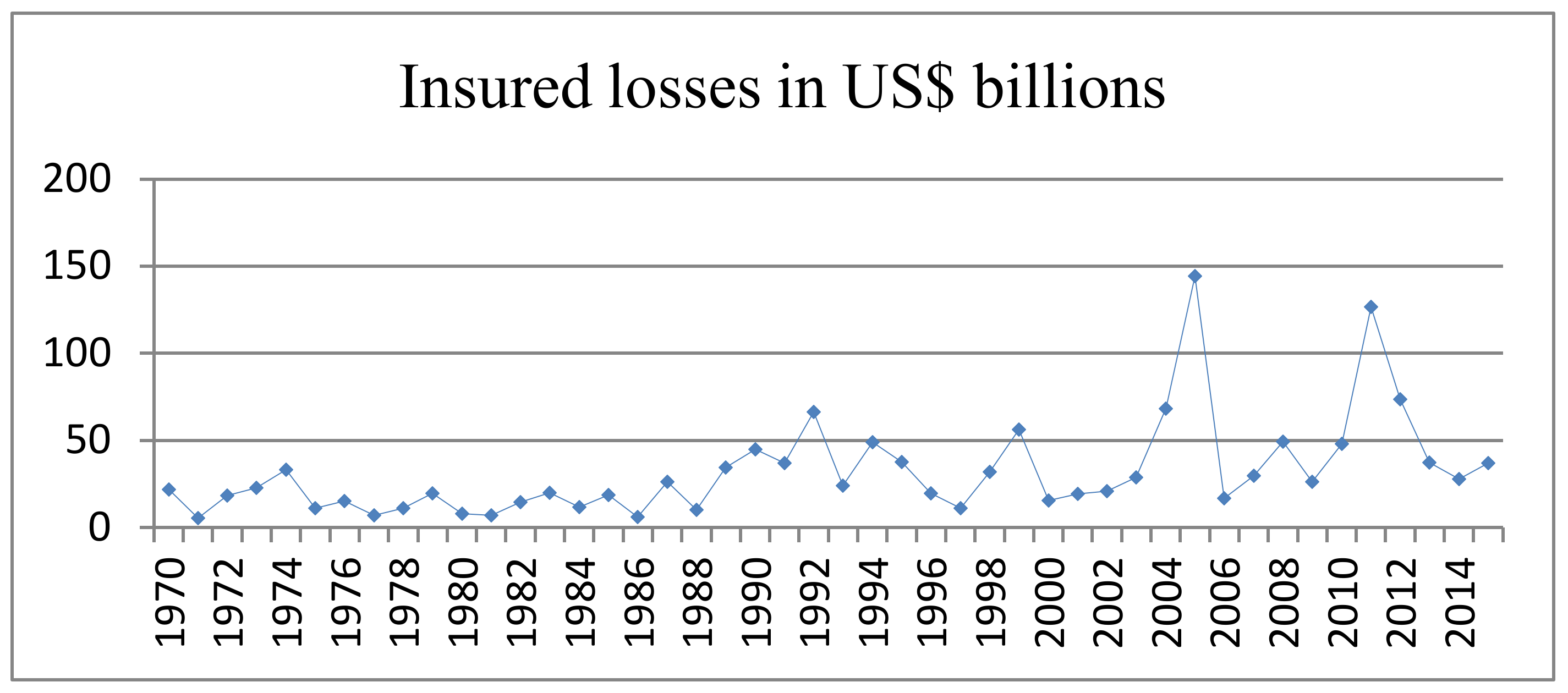
Figure 1. Trends in global insured losses from 1970 to 2015.
Sustainability 14 10617 g001
Figure 2. The plot of general agricultural production.
Sustainability 14 10617 g002
Publisher’s Note: MDPI stays neutral with regard to jurisdictional claims in published maps and institutional affiliations.