Abstract
A wireless sensor network (WSN) is a distributed network system composed of a great many sensor nodes that rely on self-organization. The random deployment of WSNs in city planning often leads to the problem of low coverage of monitoring areas. In the construction of smart cities in particular, a large number of sensor nodes need to be deployed to maintain the reception, processing, and transmission of data throughout the city. However, the uneven distribution of nodes can cause a lot of wasted resources. To solve this problem, this paper proposes a WSN coverage optimization model based on an improved marine predator algorithm (IMPA). The algorithm introduces a dynamic inertia weight adjustment strategy in the global exploration and local exploitation stages of the standard marine predator algorithm to balance the exploration and exploitation capabilities of the algorithm and improve its solution accuracy. At the same time, the improved algorithm uses a multi-elite random leading strategy to enhance the information exchange rate between population individuals and improve the algorithm’s ability to jump out of the local optimum. The optimization experiment results of 11 benchmark test functions and part of the CEC2014 test functions show that the optimization performance of the improved algorithm is significantly better than the standard marine predator algorithm and other algorithms in the literature. Finally, the improved algorithm is applied to the WSN coverage optimization problem. The simulation results demonstrate that the IMPA has a better coverage rate than other metaheuristic algorithms and other improved algorithms in the literature for solving the WSN coverage optimization problem.
1. Introduction
With the continuous development of internet technology, artificial intelligence, and 5G technology, the Internet of Things has become a hot research topic in the current technology field. As one of the core supporting technologies of the Internet of Things, wireless sensor networks play a supporting role in the Internet of Things. Wireless sensor networks (WSNs) are networks in which multiple homogeneous sensor nodes are interconnected and communicate for information transmission [1,2]. They use wireless communication to complete the target monitoring and information transmission of the environment. WSNs are widely used in aviation [3], environmental [4], medical [5], industrial [6], and other fields due to their advantages of low cost, versatility and easy deployment. In recent years, the fields of smart transportation [7], smart homes [8], and smart cities [9] have also achieved large-scale applications. However, the traditional random deployment method can lead to large-scale node coverage gaps and high-density overlapping coverage in the target area, which directly affects the detection quality of the target area and causes resource waste. Therefore, investigating ways to adaptively deploy sensor nodes in WSNs and make the distribution of sensor nodes more uniform and the coverage of nodes higher is of great significance for reducing the cost of constructing WSNs and improving the quality of network services.
In recent years, researchers have proposed many metaheuristic algorithms inspired by the behaviour of natural biological groups and the laws of physical phenomena. These algorithms are widely used in the node deployment optimization problem of WSNs because of their simple principles, few parameters, and easy implementation. The metaheuristic algorithms commonly used to solve WSN coverage problems include the bee algorithm (BA) [10], whale optimization algorithm (WOA) [11], particle swarm optimization (PSO) [12], grey wolf optimization algorithm (GWO) [13], black hole algorithm (BHA) [14], butterfly optimization algorithm (BOA) [15], genetic algorithm (GA) [16], etc. In addition, to improve the coverage rate of WSNs, many scholars have proposed improved metaheuristic algorithms. Hu et al. proposed an improved grey wolf optimization algorithm (IGWO) to enhance the WSN coverage rate [17]. Zhu et al. proposed a hybrid strategy weed algorithm (LRDE_IWO) to solve the problem of the dense and sparse distribution of nodes in the monitoring area [18]. Wang et al. proposed a virtual force-Lévy-embedded grey wolf optimization (VFLGWO) algorithm to effectively solve uneven WSN coverage problems [19]. He et al. optimized the deployment of WSN nodes by using the improved sine–cosine optimization algorithm, and the coverage rate was improved compared with the original sine–cosine algorithm [20]. The above research shows that it is feasible to use a metaheuristic algorithm to optimize WSN node deployment, but the node coverage still needs to be improved.
The marine predator algorithm (MPA) is a new metaheuristic algorithm proposed by Faramarzi et al. in 2020 [21]. The algorithm is inspired by the movement of marine predators and their prey, that is, marine predators search for food sources through Lévy motion or Brownian motion. The MPA has been successfully applied in many fields due to advantages such as its simple operation, few parameters to be adjusted, and strong stability. For example, Abd-Elaziz et al. applied the MPA to the multilevel image segmentation problem and obtained satisfactory segmentation results [22]. Abdel-Baset et al. used the MPA to improve the parameter estimation of photovoltaic models [23]. Eid et al. used the MPA to optimize active and reactive power resources in distribution networks, to minimize the total losses and total voltage deviations, and to improve the distribution system’s overall performance [24]. However, few scholars have proposed an improved MPA to solve the WSN coverage optimization problem. Hence, this paper proposes an improved MPA to solve the WSN coverage optimization problem. The proposed algorithm uses the dynamic inertia weight adjustment strategy to balance the exploration and exploitation capabilities of the algorithm. In addition, the improved algorithm uses the multi-elite random leading strategy to enhance the information exchange rate between population individuals. In summary, the main contributions of this paper are as follows:
- An improvement in the efficiency of a powerful metaheuristic method named MPA is investigated to solve the WSN coverage optimization problem.
- An improved marine predator algorithm (IMPA), combined with a dynamic inertia weight adjustment strategy and multi-elite random leading strategy, is developed to improve the ability of the standard MPA to handle complex problems. The performance of the IMPA is evaluated on 11 benchmark test functions and part of the CEC2014 test functions.
- The proposed IMPA is applied to solve the WSN coverage optimization problem. The results are compared with those of other metaheuristic algorithms and improved algorithms in the literature.
The remainder of the paper is organized as follows: Section 2 describes the WSN coverage problem mathematically. Section 3 describes the details of the proposed IMPA, along with the mathematical model and computational process. Section 4 analyses the experimental results of the proposed IMPA. Section 5 analyses the effectiveness and feasibility of the proposed IMPA in solving the WSN coverage problem. The conclusion of this work is provided in Section 6.
2. WSN Coverage Model
Assume that WSN randomly deploys N isomorphic sensor nodes on a two-dimensional plane sensing field with a size of M = × , and each sensor node has the same sensing radius and communication radius . The wireless sensor node set is positioned as L = {, , …, }, and the coordinates of are (, ), i∈{1, 2, …, N}. To better calculate the node coverage, the two-dimensional plane M is discretized into m × n grid points to be covered, and the geometric center of the grid is the coverage target point = (, ), j∈{1, 2, …, m × n}. If the distance between grid point and any node in the target area is less than or equal to the perception radius , the grid point is considered to be completely covered by the WSN. The Euclidean distance between sensor node and grid point is as follows:
The probability that grid node is covered by sensor node is defined as:
where is the perceptual error radius, and λ is the perceptual attenuation coefficient.
In this area, any grid can be covered by multiple sensor nodes at the same time. The mathematical model of the joint coverage probability is as follows:
where L is the set of all sensor nodes in the target area. The total coverage of the target area is defined as the ratio of the number of grids covered by the node set L to the total number of grids in the area. Therefore, the mathematical model of coverage is defined as:
Formula (4) shows that the WSN coverage optimization goal is to deploy a certain number of sensor nodes in a reasonable area to achieve the maximum . Therefore, this paper applies the proposed improved marine predator algorithm to obtain the optimal value of to improve the coverage of the WSN.
3. Improved Marine Predator Algorithm
3.1. Standard Marine Predator Algorithm (MPA)
The MPA is a metaheuristic algorithm proposed based on the hunting behaviour of marine predators. Similar to other metaheuristic algorithms, the MPA population initialization uses the random initialization of the prey position. Its mathematical model is shown in Formula (5):
where and are the upper and lower boundaries of the search space, respectively, and rand is a random number between [0, 1]. According to the movement modes of predators and prey, the optimization process of the MPA is divided into three phases. The specific operation process is as follows:
Phase 1: At the beginning of the algorithm iteration, the predator moves faster than the prey, and so this stage aims to explore the search space and find the prey. Therefore, its mathematical model is shown in Formula (7):
where t is the current number of iterations, is the maximum number of iterations of the algorithm, stepsize is the moving step size, is the Brownian walk random vector obeying the normal distribution, is the elite matrix constructed by the top predator, is the prey matrix with the same dimension as the elite matrix, ⨂ denotes the elementwise multiplication, P is a constant value of 0.5, and R is a random number between [0, 1].
Phase 2: In this stage, the population is divided into two parts, one part is exploited by prey using a Lévy walk, and the other part is the exploration by the predator using Brownian motion. The specific mathematical models are as shown in Formulas (9) and (11):
where is the random vector serving Lévy’s motion, CF is the adaptive parameter that controls the predator’s moving step, and its mathematical model is shown in Formula (12):
Phase 3: In the last third iteration, this phase is mainly the exploitation phase. The predator mainly approaches the prey through Lévy’s motion. The mathematical model is shown in Formula (14):
In addition to the above phases, the MPA also considers the formation of eddy currents and the influence of Fish Aggregating Devices (FADs), and its mathematical model is shown in Formula (15):
where is the probability of FADs influencing the optimization process, U is a binary array with values 0 and 1, r is a random number between [0, 1], and the subscripts and are the random indices of the prey matrix.
3.2. Improved Marine Predator Algorithm (IMPA)
3.2.1. Multi-Elite Random Leading Strategy
From the position update formula of the standard MPA, it can be seen that the moving step length of marine predators to capture prey is controlled by the elite matrix constructed with the top predator. Although the top predator can lead the population to quickly move towards the optimal solution area, when the top predator falls into the local optimum, the chain rule will guide other individuals of the population to gather towards the local optimum area, which leads to the premature convergence of the algorithm. To enhance the diversity of algorithms, this paper proposes a multi-elite random leading strategy inspired by the equilibrium pool of the equilibrium optimization algorithm [25]. In simple terms, the elite pool is constructed by calculating the population fitness value to select the current optimal top three individual positions and an average position of the elite group. As shown in Figure 1, the position update of the candidate solution can be guided by the current three optimal individual positions or the average position of the elite group. The first three individuals help to improve the exploration ability of the algorithm and the last average elite individual helps to improve the exploitation ability of the algorithm, avoiding to a certain extent the problem of the MPA falling into a local optimum due to insufficient diversity in the late iteration. The mathematical model for the elite pool construction is shown in Formulas (16) and (17):
where , and are the top three individuals with the best population fitness values in the t-th iteration, respectively, denotes the average position of the elite population and N is the population size.
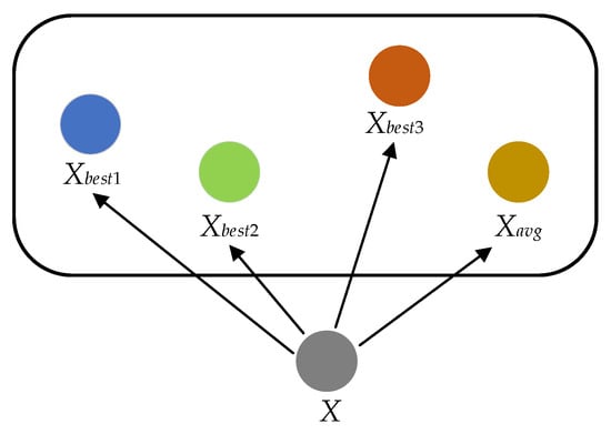
Figure 1.
Elite pool strategy diagram.
To improve the diversity of the population, elite individuals are randomly selected from the elite pool constructed above to guide and update the candidate solution positions. The mathematical model is as follows:
where λ is the contraction factor, and are random numbers between [0, 1], respectively, and is a randomly selected individual in the elite pool.
Although using a multi-elite random leading strategy can effectively improve the algorithm’s solution accuracy and avoid the algorithm falling into a local optimum, there is no way to ensure whether each updated individual position is better than the original individual position. Therefore, we use the greedy selection strategy to retain the current dominant individuals, and its mathematical model is as follows:
3.2.2. Dynamic Inertia Weight Adjustment Strategy
The disadvantage of metaheuristics lies in effectively balancing the global exploration and local exploitation capabilities of the algorithm [26]. To improve the performance of the MPA, this paper adopts a nonlinear inertia weight factor based on the combination of the cosine function and exponent, inspired by the inertia weight dynamic balance global and local search ability of the literature [27]. In the early stage of algorithm iteration, marine predators need strong global exploration capabilities to ensure that predators can search for prey more widely in the search space. Therefore, we provide a larger weight to make the predator traverse the entire search space with a large step size, which is beneficial for the predator to quickly find the prey and speed up the algorithm convergence. In the late stage of the algorithm iteration, the predator needs to have a strong local development ability to ensure that the predator can better capture the prey. Therefore, we provide a smaller weight to help predators acquire more prey sources in greater depth and to improve the convergence accuracy of the algorithm. The mathematical model of the nonlinear dynamic inertia weight w is shown in Formula (21):
where t is the current number of iterations, and is the maximum number of iterations. The inertia weight factor is introduced into the MPA, and the position update formula in the early stage of the algorithm iteration is as follows:
The position update formula in the later iteration of the MPA is as follows:
3.2.3. Detailed Steps for the Improved Marine Predator Algorithm
Combining the above improvement methods, the specific flow of the IMPA proposed in the paper is shown in Figure 2. The steps of the IMPA are described as follows:
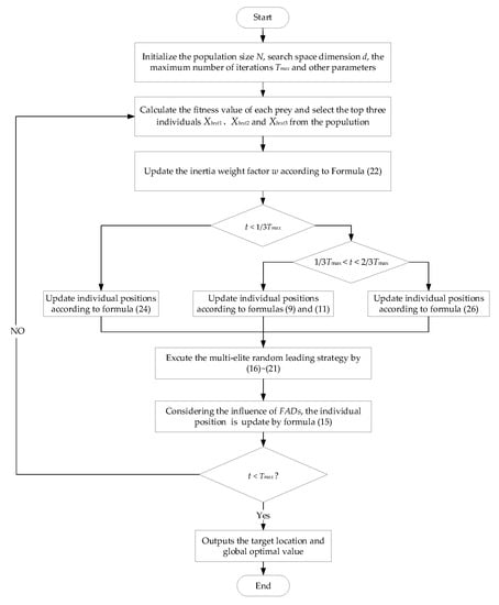
Figure 2.
Flow chart for the proposed IMPA.
- Step 1:
- Randomly initialize the population and set relevant parameters, including population size N, dimension, maximum number of iterations , FADs, etc.
- Step 2:
- Calculate the fitness value of each prey in the population and record the current optimal top three individual positions.
- Step 3:
- Update the nonlinear inertia weight factor w, and parameters such as parameters CF and .
- Step 4:
- According to the iteration conditions, the prey position and the moving step are updated by Formulas (9), (11), (24) and (26), respectively.
- Step 5:
- According to Formulas (16)–(21), execute the multi-elite random leading strategy to update the individual position of the prey.
- Step 6:
- Considering the influence of FADs, use Formula (15) to further update the position and keep the optimal individual position.
- Step 7:
- Judge whether the algorithm meets the end condition; if so, the algorithm ends and outputs the optimal individual fitness value; otherwise, return to Step 2.
3.2.4. Time Complexity Analysis of Improved Marine Predator Algorithm
The time complexity of the IMPA is mainly composed of the total time complexity of the standard MPA, the dynamic inertia weight adjustment strategy, and the multi-elite random leading strategy. Assuming that the population size of the MPA is N, the search space dimension is d, and the maximum number of iterations is , the total time complexity of the standard MPA is O(N × d × ). The IMPA is improved from the standard MPA. First of all, if the time required to update the nonlinear inertia weight factor is , the time complexity of introducing the weight factor w into the MPA to update the individual position is O(N × d × + ) = O(N × d × ). Then, the time required to calculate the fitness value of the population individuals and screen the first three optimal individual positions is , the time required to randomly select elite individuals from the elite pool is , and the time required to compare the fitness values of new and old individuals using the superiority and inferiority mechanisms is . The time complexity of introducing a multi-elite random leading strategy is O(N × d × + + + ) = O(N × d × ). Therefore, the total time complexity of the IMPA is O(N × d × ) + O(N × d × ) + O(N × d × ) = O(N × d × ).
Based on the above analysis, the time complexity of the IMPA proposed in this paper is consistent with that of the standard MPA, indicating that the improved strategy proposed in this paper for the defects of the standard MPA does not increase the computational burden.
4. The Simulation Results
4.1. Experimental Environment and Parameter Setting
The experimental running environment is a 64-bit Windows 10 operating system, the CPU is Intel Core i5-7200U, the main frequency is 2.6 GHz, and the memory is 4 GB. The algorithm is written using MATLAB R2018a. To fully verify the effectiveness of the IMPA, this section selects 11 benchmark functions with different characteristics for experimental simulation. Among them, f1~f5 are unimodal test functions, f6~f10 are multimodal test functions, and f11 is a fixed low-dimensional test function. The specific information of the benchmark function is shown in Table 1. The parameter settings of each comparison algorithm are shown in Table 2.

Table 1.
The benchmark test function.

Table 2.
Set the experimental parameters of each algorithm.
4.2. Experimental Results and Analysis
In order to fully verify the effectiveness of the proposed IMPA, the IMPA is compared with other classical metaheuristic algorithms, such as the sine–cosine algorithm (SCA) [28], tunicate swarm algorithm (TSA) [29], mayfly algorithm (MA) [30], and equilibrium optimizer algorithm (EO) [31]. To ensure the fairness of the algorithm comparison, the population size N = 30, and the maximum number of iterations = 500. To avoid the contingency of running the results of the algorithms, all the comparison algorithms were independently run 30 times on 11 benchmark functions, and the mean, standard deviation, and average time consumed were taken as the final evaluation indicators. The detailed comparison data are shown in Table 3. In the table, Mean is the average optimal fitness value, Std is the standard deviation, and Time(s) is the average time consumed.

Table 3.
Comparison of the optimization performance of each algorithm on the benchmark function.
The data in Table 3 show that the IMPA can better balance the global exploration and local exploitation capabilities of the algorithm under the conditions of 30-dimensional and fixed-dimensional dimensions. For the unimodal functions f1~f5, the IMPA can solve the theoretical optimal value on the functions f1~f4. When solving the f5 function, the IMPA easily falls into the same local extreme value space as the other algorithms, but the convergence accuracy and standard deviation are better than the other five algorithms. When solving multimodal functions f6~f10 and fixed low-dimensional functions, the IMPA can solve the theoretical optimal value on functions f6 and f8~f10. For functions f7 and f11, although the IMPA fails to solve the theoretical optimal value, the solution accuracy is much higher than that of the other algorithms and the standard deviation is the smallest, indicating that the integration of the dynamic inertia weight adjustment strategy can balance the global exploration and local exploitation of the algorithm’s ability. It effectively pushes the predator to move towards the prey source, which improves the solution accuracy and stability of the algorithm. In addition, the average time consumed shown in Table 3 demonstrates that the average time consumption of the proposed algorithm is almost close to the standard MPA. Therefore, the time complexity of our proposed IMPA does not improve.
In order to more intuitively reflect the convergence performance of each algorithm, Figure 3 shows the comparison of the average curves of the IMPA and the EO algorithm, SCA, TSA, and MA on some benchmark functions. The experimental parameters are the same as above. To facilitate the observation of the convergence, the ordinate in the figure is the logarithm of base 10. Figure 3a–f shows that with the increase in the number of iterations, the convergence speed of the IMPA is faster and the convergence accuracy is higher than that of the standard MPA, which shows that the use of the multi-elite random selection leading strategy can effectively enrich species diversity. In addition, it can be seen from the figure that the IMPA does not appear stagnant in the late iteration, and the convergence speed and solution accuracy are much higher than those of other algorithms. This is mainly due to the multi-elite random leading strategy to enrich the diversity of the population and the inertia weight adjustment strategy to dynamically balance global exploration and local exploitation. Combining the experimental data results in Table 3 and the average convergence curves in Figure 3a–f, the effectiveness of the IMPA can be concluded. Although on the function f11, the average fitness value obtained by the IMPA is similar to other algorithms, the IMPA has more prominent comprehensive optimization ability in general.
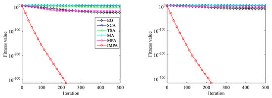

Figure 3.
Partial convergence curves of the proposed IMPA and other metaheuristic algorithms on the benchmark test functions: (a) Convergence curve of f1; (b) Convergence curve of f3; (c) Convergence curve of f5; (d) Convergence curve of f7; (e) Convergence curve of f9; (f) Convergence curve of f11.
4.3. Performance Analysis of Improved Algorithm in High Dimensions
Given the limited space, this section selects two single-peak test functions (f1, f2) and two multipeak test functions (f7, f9). The dimensionality is varied in 50-dimensional increments from 50 to 300 dimensions, and the mean and average rate of change of the algorithm’s solutions are used as evaluation metrics. To avoid the contingency of the experimental results, the proposed IMPA and the standard MPA were run independently 30 times, and the average value of the fitness with the function dimension was recorded. The parameter settings are the same as in Section 4.2, and the experimental results are shown in Table 4. The mathematical model for the average rate of change (ARC) is as follows:

Table 4.
Comparison of IMPA and MPA on the mean value of optimization functions in different dimensions.
It can be seen from Table 4 that with the increase in dimension, the objective function is also complicated, but the average value of the IMPA solution remains unchanged. Especially for functions f1, f2, and f9, the IMPA solution’s accuracy can maintain the theoretical optimum value of 0. However, with the increase of dimension, the solution accuracy of the standard MPA will increase significantly. For function f7, the IMPA fails to find the theoretical optimum of 0, but the average rate of change with increasing dimensionality is 0, which is much lower than the average rate of change of the standard MPA.
To intuitively reflect the change of the average value of IMPA and MPA with the increase of the function dimension, Figure 4 presents the curve graph of the average value change of the two algorithms in different dimensions. Figure 4 shows that the solution accuracy of standard the MPA increases monotonically with increasing dimensions, and the increase is more obvious. However, the solution accuracy of IMPA does not increase with the increase of dimensions, which means that IMPA also has a good solution effect for complex high-dimensional multi-extremal functions. Therefore, the use of the multi-elite random selection leading strategy and dynamic inertia weight adjustment strategy can lead the MPA to have a better solution effect, which further verifies the possibility and effectiveness of the proposed algorithm.
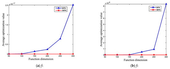
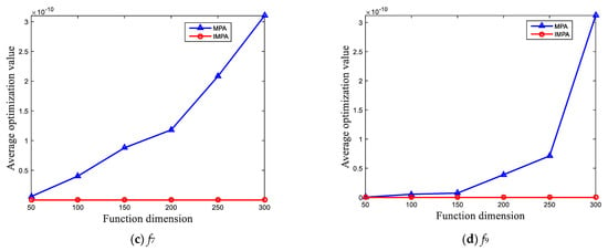
Figure 4.
Function optimization with function dimension change curves: (a) Change curves of f1; (b) Change curves of f2; (c) Change curves of f7; (d) Change curves of f9.
4.4. Comparison with the Latest Improved Marine Predator Algorithm
To highlight the competitiveness of IMPA, this section compares the IMPA with the state-of-the-art improved marine predator algorithms ODMPA [32] and LEO-MPA [33]. The experiment selects 11 benchmark functions in Section 4.2; the population size N = 30, the search space dimension d = 30, and the maximum number of iterations = 500. The parameter settings of each algorithm refer to the original literature and we let each algorithm run independently 30 times. The experimental results are shown in Table 5. In the table, “—” represents missing data in the literature.

Table 5.
Comparison results with the latest improved MPA.
Table 5 shows that the IMPA also has significant advantages over the two latest improved marine predator algorithms. Specifically, for unimodal functions f1~f4, the IMPA is far superior to the other two algorithms in terms of solution effect and stability. For function f5, because its shape is similar to that of a paraboloid, there are a large number of local extreme points, so neither the IMPA nor other algorithms can find the theoretical optimal value. However, the mean and standard deviation of the IMPA is one order of magnitude higher than those of the ODMPA and LEO-MPA and have a better ability to jump out of the local optimum. For the multi-peaked functions f6 to f8, the IMPA is comparable to the other two algorithms. For solving the fixed-dimensional function f11, the standard deviation of the IMPA is slightly inferior to that of the LEO-MPA. In general, from the two indicators of the mean and standard deviation, the overall optimization performance of the IMPA is much higher than that of the other two improved algorithms, which further verifies the superiority of the IMPA.
4.5. Experimental Analysis of CEC2014 Test Function
To further verify the advantages of the IMPA’s optimization performance, this section selects the IMPA and five other algorithms to perform optimization performance tests on part of the CEC2014 test function sets [34] with complex features, including the standard MPA, TSA, EO algorithm, MA and improved HEGMPA [35]. The specific characteristics of the function are shown in Table 6. To ensure the fairness of pairs, the population size is N = 30, the maximum number of iterations = 1000, and the search space dimension is d = 30. Each algorithm was independently run 30 times and its mean and standard deviation were recorded. The experimental results are shown in Table 7.

Table 6.
CEC2014 test functions.

Table 7.
Comparison of optimization results of CEC2014.
It can be seen from Table 7 that the MPA performs well on the unimodal function CEC03, and the solution accuracy of the IMPA is slightly inferior to the MPA and HEGMPA. This is because the IMPA needs to perform more parameter calculations when it randomly selects elites, which reduces the solution accuracy, but the optimization performance of the IMPA is better than that of the remaining three algorithms. On multimodal functions (CEC05, CEC08, CEC11) and hybrid functions (CEC19, CEC20), the IMPA is closer to the theoretical optimum than the other four algorithms. Especially on the functions CEC05 and CEC20, the IMPA basically solves to the theoretical optimal value. On the composition functions (CEC25, CEC27, CEC28, CEC30), the solution accuracy of the IMPA is much higher than that of the other four algorithms and the standard deviation is 0, indicating that the IMPA has the best stability. In summary, the IMPA is better than the other four algorithms in its ability to search for complex feature functions, which shows that it is feasible and effective to integrate the multi-elite random leading strategy and the dynamic inertia weight adjustment strategy into the marine predator algorithm in this paper.
5. Coverage Optimization in Wireless Sensor Networks (WSNs)
To verify the feasibility and effectiveness of the proposed IMPA for WSN node coverage optimization, two experiments were performed. Experiment 1 compares the effect of the IMPA with EO, SCA and the original MPA. Experiment 2 compares the IMPA with the improved grey wolf optimization (IGWO) [17], invasive weed algorithm (IWO) [18], improved hybrid strategy weed algorithm (LRDE_IWO) [18], Lévy-embedded grey wolf optimization (LGWO) [19] and virtual force-Lévy-embedded grey wolf optimization (VFLGWO) [19]. In the experiments, the parameters are set the same as in the literature [17].
Assume that 40 sensor nodes are deployed in the sensing field of the target area M = 50 × 50 m, the perceived radius = 10 m, the communication radius = 20 m, and the maximum number of iterations = 500. The specific parameters are shown in Table 8.

Table 8.
WSN coverage parameter settings.
5.1. Comparison with Other Standard Metaheuristics
To verify the effectiveness of IMPA in solving the WSN coverage problem, the IMPA, EO algorithm, SCA and the original MPA are simulated. The experimental data are shown in Table 9. Figure 5 shows the node coverage graph of the proposed IMPA, random deployment, and optimization of each algorithm.

Table 9.
Comparison of the average coverage of each algorithm optimization.
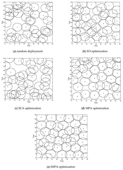
Figure 5.
Node coverage graph of each algorithm: (a) Random deployment node coverage graph; (b) EO-optimized node coverage graph; (c) SCA-optimized node coverage graph; (d) MPA-optimized node coverage graph; (e) IMPA-optimized node coverage graph.
As seen from Table 9, the coverage rate optimized by the IMPA reaches 93.72%. At the same time, the coverage rate of the IMPA is improved by 19.10%, 4.28%, 16.84%, and 4.91% compared with the random deployment, EO algorithm, SCA algorithm, and the original MPA, respectively. From Figure 5a,c, the middle region optimized by random deployment and the SCA algorithm has a large range of coverage blank phenomena. Figure 5b,d show that the upper left region optimized by the EO algorithm and the MPA has a serious overlap phenomenon. In Figure 5e, the regional node coverage optimized by the IMPA is more uniform and less redundant, and the full coverage of the target area is approximately achieved, which effectively improves the random deployment node coverage vulnerability and the MPA-optimized node coverage aggregation defect.
To further explore the influence of the number of sensor nodes on the WSN-optimized node coverage, simulation experiments were carried out on different sensor nodes for each algorithm (random deployment, MPA and IMPA) in the target area. The number of isomorphic sensor nodes is set to 35, 40, 45, 50, and 55, and the other parameters are consistent with Table 8. The variation trend of the coverage ratio of different algorithms with the number of nodes is shown in Figure 6.
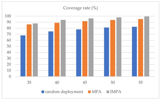
Figure 6.
Comparison of coverage of different numbers of nodes.
As shown in Figure 6, the proposed algorithm is superior to the random deployment and the MPA in the coverage rate of wireless sensor network nodes with different numbers of nodes, and the IMPA almost approaches a 100% coverage rate when there are 55 nodes. This shows that the two strategies of the IMPA can effectively improve the probability of escaping from a local optimum and balance the ability of global exploration and local exploitation, thereby improving the effective coverage rate of the WSN nodes.
5.2. Comparison with the Latest Improved Algorithm
To highlight the competitiveness of the IMPA in solving the WSN coverage problem, Table 10 depicts the comparison results of the IMPA with other algorithms in the literature, including IGWO [17], IWO [18], LRDE_IWO [18], LGWO [19], and VFTGWO [19]. Table 10 shows that the coverage rate of the IMPA is slightly inferior to the LRDE_IWO algorithm. However, compared with other four algorithms, the IMPA still has an advantage. Therefore, the IMPA has certain practicability for improving the WSN coverage problem.

Table 10.
Comparison of the average coverage of the latest improved algorithm.
6. Conclusions
To effectively improve the node deployment coverage rate of wireless sensor networks, an improved marine predator algorithm, termed IMPA, was proposed. It combines a dynamic inertia weight adjustment strategy and a multi-elite random leading strategy to better improve the coverage rate of WSNs in monitoring areas and the reduction of resource waste. Eleven benchmark functions with different features and partial CEC2014 test functions were tested and compared with existing metaheuristics and improved algorithms. The experimental results demonstrated that the IMPA had better stability and optimization performance than other algorithms. Finally, the IMPA was applied to a WSN coverage optimization problem. The simulation results showed that the IMPA coverage was higher than that of IGWO, IWO, LGWO, VFTGWO, and other metaheuristic algorithms.
In future research, we aim to consider additional optimization objectives based on the WSN coverage optimization problem; for example, predicting the energy consumption of nodes. In other words, we intend to investigate how to effectively adjust the size of the perceived radius of sensor nodes in order to reduce the sensing redundancy of the monitored area, thereby achieving the objective of extending the network life cycle.
Author Contributions
Conceptualization, Q.H. and D.Z.; methodology, Q.H., Z.L. and D.Z.; software, Z.L.; validation, Q.H. and Z.L.; formal analysis, Q.H. and D.Z.; writing—original draft preparation, Q.H.; writing—review and editing, Z.L., L.Y. and S.L.; resources, Q.H.; data curation, Z.L.; visualization, L.Y. and S.L. All authors have read and agreed to the published version of the manuscript.
Funding
The research was funded by the National Natural Science Foundation of China “Research on the Evidence Chain Construction from the Analysis of the Investigation Documents (62166006)”, the National Natural Science Foundation of China “Rural spatial restructuring in poverty-stricken mountainous areas of Guizhou based on spatial equity: A case study of Dianqiangui Rocky Desertification Area (41861038)”, and Guizhou Provincial Science and Technology Projects (Guizhou Science Foundation-ZK [2021] General 335).
Institutional Review Board Statement
Not applicable.
Informed Consent Statement
Not applicable.
Data Availability Statement
Not applicable.
Conflicts of Interest
The authors declare no conflict of interest.
References
- Ni, Q.J.; Du, H.M.; Pan, Q.Q.; Cao, C.; Zhai, Y.Q. An improved dynamic deployment method for wireless sensor network based on multi-swarm particle swarm optimization. Nat. Comput. 2017, 16, 5–13. [Google Scholar] [CrossRef]
- Tabibi, S.; Ghaffari, A. Energy-efficient routing mechanism for mobile sink in wireless sensor networks using particle swarm optimization algorithm. Wirel. Pers. Commun. 2019, 104, 199–216. [Google Scholar] [CrossRef]
- Stankunas, J.; Rudinskas, D.; Lasauskas, E. Experimental research of wireless sensor network application in aviation. Elektron. Elektrotech. 2011, 111, 41–44. [Google Scholar] [CrossRef]
- Teng, Z.J.; Pang, B.H.; Sun, M.Y.; Xie, L.Y.; Guo, L.W. A Malicious Node Identification Strategy with Environmental Parameters Optimization in Wireless Sensor Network. Wirel. Pers. Commun. 2021, 117, 1143–1162. [Google Scholar] [CrossRef]
- Shen, L.; Ma, J.; Liu, X.; Miao, M. A provably secure aggregate signature scheme for healthcare wireless sensor networks. J. Med. Syst. 2016, 40, 1–10. [Google Scholar] [CrossRef]
- Yoo, S.; Kim, T. Industrial Wireless Sensor Networks: Protocols and Applications. Sensors 2020, 20, 5809. [Google Scholar] [CrossRef]
- Zhang, K.; Jia, H.; Lv, H. Coverage-enhancing approach in multimedia directional sensor networks for smart transportation. Multimed. Tools Appl. 2016, 75, 17593–17615. [Google Scholar] [CrossRef]
- Li, M.; Lin, H.J. Design and implementation of smart home control systems based on wireless sensor networks and power line communications. IEEE Trans. Ind. Electron. 2014, 62, 4430–4442. [Google Scholar] [CrossRef]
- Wang, H.; Xu, L.W.; Lin, W.Z.; Xiao, P.P.; Wen, R.H. Physical layer security performance of wireless mobile sensor networks in smart city. IEEE Access 2019, 7, 15436–15443. [Google Scholar] [CrossRef]
- Khalaf, O.I.; Abdulsahib, G.M.; Sabbar, B.M. Optimization of wireless sensor network coverage using the Bee Algorithm. J. Inf. Sci. Eng. 2020, 36, 377–386. [Google Scholar]
- Yue, Y.; You, H.; Wang, S.; Cao, L. Improved whale optimization algorithm and its application in heterogeneous wireless sensor networks. Int. J. Distrib. Sens. Netw. 2021, 17, 15501477211018140. [Google Scholar] [CrossRef]
- Ling, H.F.; Zhu, T.; He, W.X.; Luo, H.C.; Wang, Q.; Jiang, Y. Coverage optimization of sensors under multiple constraints using the improved PSO algorithm. Math. Probl. Eng. 2020, 2020, 8820907. [Google Scholar] [CrossRef]
- Zhang, Y.; Cao, L.; Yue, Y.G.; Cai, Y.; Hang, B. A novel coverage optimization strategy based on grey Wolf algorithm optimized by simulated annealing for wireless sensor networks. Comput. Intell. Neurosci. 2021, 2021, 6688408. [Google Scholar] [CrossRef]
- Pan, J.S.; Chai, Q.W.; Chu, S.C.; Wu, N. 3-D terrain node coverage of wireless sensor network using enhanced black hole algorithm. Sensors 2020, 20, 2411. [Google Scholar] [CrossRef]
- Ma, D.; Duan, Q. A hybrid-strategy-improved butterfly optimization algorithm applied to the node coverage problem of wireless sensor networks. Math. Biosci. Eng. 2022, 19, 3928–3952. [Google Scholar] [CrossRef]
- Bouzid, S.E.; Seresstou, Y.; Raoof, K.; Omri, M.N.; Mbarki, M.; Dridi, C. MOONGA: Multi-objective optimization of wireless network approach based on genetic algorithm. IEEE Access 2020, 8, 105793–105814. [Google Scholar] [CrossRef]
- Hu, X.P.; Cao, J. Improved grey wolf optimization algorithm for WSN node deployment. Chin. J. Sens. Actuators 2018, 31, 753–758. [Google Scholar]
- Zhu, F.; Wang, W. A Coverage Optimization Method for WSNs Based on the Improved Weed Algorithm. Sensors 2021, 21, 5869. [Google Scholar] [CrossRef]
- Wang, S.; Yang, X.; Wang, X.; Qian, Z. A virtual force algorithm-Lévy-embedded grey wolf optimization algorithm for wireless sensor network coverage optimization. Sensors 2019, 19, 2735. [Google Scholar] [CrossRef]
- He, Q.; Xu, Q.; Wei, K. Enhanced sine cosine algorithm based node deployment optimization of wireless sensor network. J. Comput. Appl. 2019, 39, 2035–2043. [Google Scholar]
- Faramarzi, A.; Heidarinejad, M.; Mirjalili, S.; Gandomi, A.H. Marine Predators Algorithm: A nature-inspired metaheuristic. Expert Syst. Appl. 2020, 152, 113377. [Google Scholar] [CrossRef]
- Abd-Elaziz, M.; Mohammadi, D.; Oliva, D.; Salimifard, K. Quantum marine predators algorithm for addressing multilevel image segmentation. Appl. Soft Comput. 2021, 110, 107598. [Google Scholar] [CrossRef]
- Abdel-Basset, M.; El-Shahat, D.; Chakrabortty, R.K.; Ryan, M. Parameter estimation of photovoltaic models using an improved marine predators algorithm. Energy Conv. Manag. 2021, 227, 113491. [Google Scholar] [CrossRef]
- Eid, A.; Kamel, S.; Abualigah, L. Marine predators algorithm for optimal allocation of active and reactive power resources in distribution networks. Neural Comput. Appl. 2021, 33, 14327–14355. [Google Scholar] [CrossRef]
- Lan, Z.; He, Q.; Jiao, H.; Yang, L. An Improved Equilibrium Optimizer for Solving Optimal Power Flow Problem. Sustainability 2022, 14, 4992. [Google Scholar] [CrossRef]
- Guo, W.; Wang, Y.; Dai, F.; Liu, T. Alternating sine cosine algorithm based on elite chaotic search strategy. Control Decis. 2019, 34, 1654–1662. [Google Scholar]
- Chen, L.; Tian, Y.; Ma, Y. An improved grasshopper optimization algorithm based on dynamic dual elite learning and sinusoidal mutation. Computing 2022, 104, 981–1015. [Google Scholar] [CrossRef]
- Mirjalili, S. SCA: A sine cosine algorithm for solving optimization problems. Knowl. Based Syst. 2016, 96, 120–133. [Google Scholar] [CrossRef]
- Li, L.L.; Liu, Z.F.; Tseng, M.L.; Zheng, S.J.; Lim, M.K. Improved tunicate swarm algorithm: Solving the dynamic economic emission dispatch problems. Appl. Soft. Comput. 2021, 108, 107504. [Google Scholar] [CrossRef]
- Zervoudakis, K.; Tsafarakis, S. A mayfly optimization algorithm. Comput. Ind. Eng. 2020, 145, 106559. [Google Scholar] [CrossRef]
- Faramarzi, A.; Heidarinejad, M.; Stephens, B.; Mirjalili, S. Equilibrium optimizer: A novel optimization algorithm. Knowl. Based Syst. 2020, 191, 105190. [Google Scholar] [CrossRef]
- Oszust, M. Enhanced Marine Predators Algorithm with Local Escaping Operator for Global Optimization. Knowl. Based Syst. 2021, 232, 107467. [Google Scholar] [CrossRef]
- Hu, G.; Zhu, X.N.; Wei, G.; Chang, C.T. An improved marine predators algorithm for shape optimization of developable Ball surfaces. Eng. Appl. Artif. Intell. 2021, 105, 104417. [Google Scholar] [CrossRef]
- Tejani, G.G.; Savsani, V.J.; Patel, V.K.; Mirjalili, S. Truss optimization with natural frequency bounds using improved symbiotic organisms search. Knowl. Based Syst. 2018, 143, 162–178. [Google Scholar] [CrossRef]
- Sun, C.J.; Gao, F. A Tent Marine Predators Algorithm with Estimation Distribution Algorithm and Gaussian Random Walk for Continuous Optimization Problems. Comput. Intell. Neurosci. 2021, 2021, 7695596. [Google Scholar] [CrossRef]
Publisher’s Note: MDPI stays neutral with regard to jurisdictional claims in published maps and institutional affiliations. |
© 2022 by the authors. Licensee MDPI, Basel, Switzerland. This article is an open access article distributed under the terms and conditions of the Creative Commons Attribution (CC BY) license (https://creativecommons.org/licenses/by/4.0/).