Wagner’s Law vs. Keynesian Hypothesis: Dynamic Impacts

Abstract

This study analyzes the dynamics between public expenditure and economic growth in Peru for 1980Q1–2021Q4. We used quarterly time series of real GDP, public consumption expenditure, public expenditure, and the share of public expenditure to output. The variables were transformed into natural logarithms, wherein only the logarithm of public expenditure to output ratio is stationary and the others are non-stationary $I\left(1\right)$. The study of stationary time series assesses whether Wagner’s law, the Keynesian hypothesis, the feedback hypothesis, or the neutrality hypothesis is valid for the Peruvian case according to Granger causality. We found cointegration between real GDP and public expenditure, and public consumption expenditure and real GDP. Estimating error correction and autoregressive distributed lag models, we concluded that Wagner’s law and the Keynesian hypothesis are valid in the Peruvian case, expressed as dynamic processes that allow us to obtain short-run and long-run impacts, permitting the mutual sustainability of economic growth and public expenditure.

1. Introduction

In Peru, government expenditure—the nonfinancial expenditures of government in general (national government, regional governments, and local governments)—constitutes current expenditure accounts (periodic expenditures for the payment of salaries and pensions, the purchase and contracting of goods and services, as well as the transfer of resources to other public sector entities and/or to the private sector) and capital expenditure (gross capital formation and other capital expenditures) [1]. In 2021, real government expenditure increased by 5.1% over the value in the previous year (its percentage variation in 2020 amounted to 12.8). This increase was due to higher expenditure on gross capital formation and purchases of goods and services to address the health crisis generated by COVID-19. However, as a fraction of GDP, government expenditure decreased by 4.4% owing to the high percentage variation in nominal GDP (21.5%). Similarly, real expenditure on transfers declined by 16.3%, and real expenditure on salaries dropped by 1.8% [2].

During 2021, public expenditure—comprising government expenditure excluding compensation, pensions, transfers, and other capital expenditures—measured as the sum of public consumption and public investment increased at a rate of 14% owing to the growth rates of public consumption (10.6%) and public investment (24.9%). Public consumption increased the growth rate by 10.6% over the value in 2020 due to higher expenditures on the purchase of medical supplies, professional and technical services to address the health crisis, and road maintenance and upkeep (the percentage variation in public consumption was 7.8 in 2020). In addition, public investment increased by 24.9% with respect to the value in the previous year, contrasting with the −15.1 percentage variation registered in 2020. Regarding economic growth, during 2021, the percentage variation in Peruvian real GDP stood at 13.3% with respect to the value in the previous year (the percentage variation in real GDP was −11.0 in 2020 due to COVID-19) [2]. In this study, we consider public expenditure in a similar way to the studies by Aparco and Flores [3] and Peña [4]; we define public expenditure as the sum of public consumption and gross fixed capital formation (GFCF).

Ansari [5] documented that the relation between public expenditure and economic growth has been widely addressed by public finance [6,7,8,9,10,11,12,13,14,15,16,17,18], as well as by macroeconomic modeling (Some of these works include the following: [19,20,21,22]). Legrenzi and Milas [23] empirically demonstrated that the omitted variables, bureaucracy and local expenditure, in an original bivariate model between GDP and public spending support the existence of a lung-run equilibrium relationship between these four variables, in Italy. Policymakers should have a proper understanding of the relation between these variables so that they may efficiently allocate public resources to achieve the desired economic growth and prosperity, according to Kirikkaleli and Ozbeser [24]. Kumar et al. [25] argued that governments should understand the dynamics of the relation between these variables to establish a proper macroeconomic policy. As Keynes [26] had already stated, periods of recession (expansion) restrict (favor) the abilities of policymakers to stimulate the economy through fiscal measures unless the share of government expenditure to output increases (decreases). Kumar et al. [25] further indicated that the long-term estimates of the relation between public expenditure and economic growth would identify a benchmark against which to ascertain the type of fiscal policy adopted by certain governments. Moreover, identifying this relation provides a theoretical framework to formulate and judge fiscal policy adjustment plans relative to medium-term budgetary objectives.

Two essential economic approaches that analyze the long-run relationship between public expenditure and economic growth include Wagner’s law and the Keynesian hypothesis (An alternative approach to those analyzed in this paper is the so-called displacement effect developed by Peacock and Wiseman [27]) which establish a relationship between economic growth and public expenditure with opposite directions of causality; while the former considers that economic growth Granger causes public expenditure, the latter postulates the opposite [28,29]. However, as indicated below, some research results have demonstrated that economic growth and public expenditure cause each other, leading to the so-called feedback hypothesis. However, other studies have presented results of noncausality between these variables, leading to the neutrality hypothesis [30].

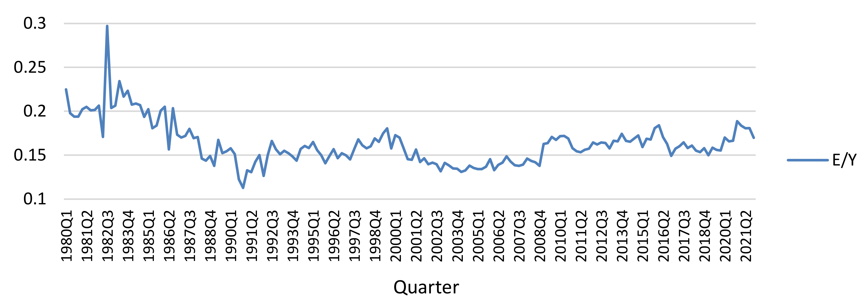
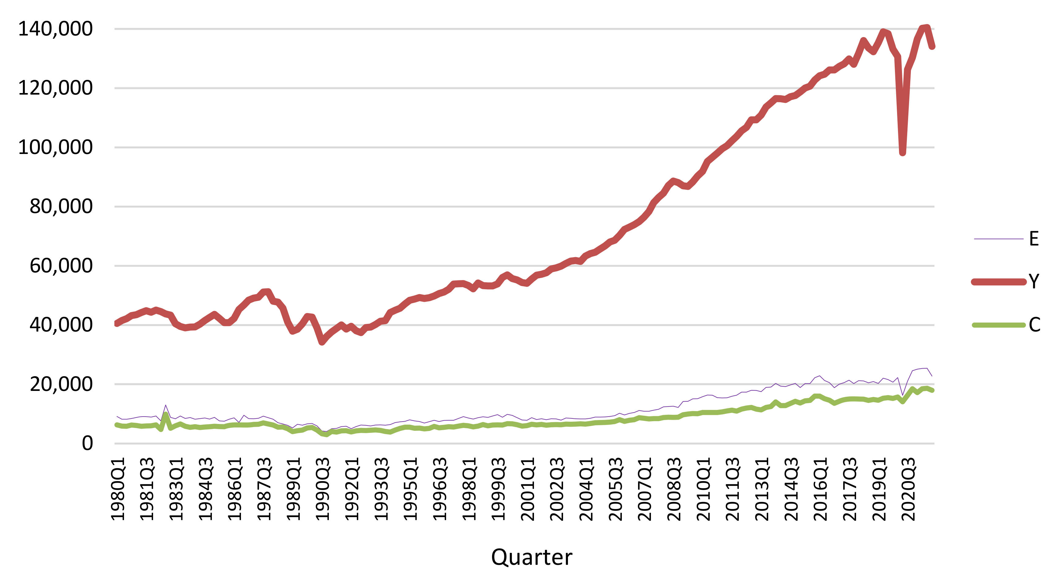
In this context, and considering evidence of an upward trend for the variables of real public consumption, real public expenditure, and real GDP since the third quarter of 1990 [31], these conditions allow to analyze the dynamics of public expenditure and economic growth in the short and long terms in Peru. In this study we use three methodologies—Granger causality, Engle–Granger cointegration, and the autoregressive distributed lag (ARDL) model—to test Wagner’s law, the Keynesian hypothesis, the feedback hypothesis, or the neutrality hypothesis. In particular, our sample corresponds to the period 1980Q1–2021Q4, with quarterly frequency for the series real GDP, real public consumption expenditure, and real public expenditure. After analyzing stationarity, our findings are the cointegration between real GDP vs. real public expenditure, and real GDP vs. real public consumption, which affirms the Peacock and Wiseman [27] and Pryor [9] estimations supporting Wagner’s law. We also ran the autoregressive distributed lag (ARDL) model for Mann’s version [16], estimating impacts that support Wagner’s law. However, taking the inverse functions for each type of model, we observe impacts that support the Keynesian hypothesis. Consequently, the purpose of this study enhances the national empirical evidence on the validity of the hypotheses concerning the relation between economic growth and public expenditure in an emerging economy.

This paper is divided into five sections. After the introduction, Section 2 describes the materials and methods used in this research, Section 3 and Section 4 presents and discusses the results, respectively. Finally, Section 5 outlines some conclusions.

Since Wagner [6] postulated the law of increasing state activities, different interpretations and formulations have been made for its empirical testing. For instance, according to Mahar and Rezende [12], and Pluta [15], Wagner’s law posits that public expenditure increases in relation to aggregate output as per capita income increases. Furthermore, Nwude and Boloupremo [32] argued that Wagner’s law analyzes the increase in the size of the public sector as a result of the economic growth of an economy. According to Arestis et al. [29], Wagner’s law states that government activities and functions expand as an economy develops and that due to this, government expenditures grow at a higher rate than that of national income so that, over time, public expenditures grow as a share of national income. According to Peña [4], Wagner’s law establishes that the public expenditure/GDP ratio is elastic with respect to GDP. According to Popescu and Diaconu (Maxim) [33], Wagner’s law stipulates that economic growth implies an increase in public expenditure.

Nwude and Boloupremo [32] sustain that “according to Wagner [6], there are three reasons to expect the expansion of public activity: (i) When the countries achieve development, they expand its administrative and protectionist functions due to the greater complexity of legal relationships and communications. Thus, increased urbanization and population density will lead to greater public expenditure on law and order and other socioeconomic regulations. (ii) When income increases, societies demand more education, entertainment and generally more public services, achieve a more equitable distribution of wealth and income. Wagner believed that the income elasticity of demand for those public services exceeded unity. (iii) Finally, the technological needs of an industrialized society require greater amounts of capital infrastructure to private sector; hence, the government has to intervene to meet those needs”.

From the Wagnerian perspective, the growth of public expenditure is a consequence of the expansion of the state produced by the economic and social progress of a country, according to Pistoresi et al. [34]. According this view, public expenditure is endogenous to economic development and national income growth Kónya and Abdullaev [35].

Furthermore, the Keynesian hypothesis considers that public expenditure causes economic growth, and that public expenditure—autonomously determined and exogenously given—represents a macroeconomic policy instrument to reduce the cyclical fluctuations of the economy in the short term and boost economic growth in the long term. From Keynes [26] perspective, an increase in public expenditure stimulates aggregate demand by generating an increase in national output. From this approach, public expenditure growth is seen as an engine that drives output growth through its multiplier effects on aggregate demand [29].

Considering the measures of government size and economic growth, according to Granger causality results with time series data or panel data, Magazzino [28], Barra et al. [36], Irandoust [37], and Nyasha and Odhiambo [30] indicated the existence of four possible hypotheses: Wagner’s law, in which unidirectional causality runs from economic growth to public expenditure [3,25,38,39,40,41,42,43,44]; the Keynesian hypothesis, in which unidirectional causality runs from public expenditure to economic growth [4,45]; feedback hypothesis, in which a bidirectional causality flow exists between economic growth and public expenditure [33,46,47,48,49,50,51]; and neutrality hypothesis, verified with variables that do not exhibit Granger causality in both directions [3,17,52].

This diversity of interpretations, along with the multiplicity of variables, methodologies, periods analyzed, and proxy measures of government size (real or nominal total public expenditure, real or nominal total public expenditure per capita, real or nominal public consumption, or ratio between total public expenditure and aggregate GDP, among others) and economic growth (real or nominal gross national product, real or nominal aggregate GDP, real or nominal GDP per capita, or real or nominal gross national product per capita, among others) has produced different types of results.

The six original modeling versions of Wagner’s law were formulated by Peacock and Wiseman [27], Gupta [7] and Michas [13], Pryor [9], Goffman [8], Musgrave [10] and Mann [16], whose models will be highlighted in this research. Mann [16] argued that the Peacock and Wiseman’s version [27] explains public expenditure as a function of gross domestic product. From Pryor [9] perspective, public consumption expenditure is a function of national income. According to Goffman [8] approach, public expenditure is a function of per capita gross domestic product. In addition, Musgrave [10] version indicated that the per capita gross domestic product explains the share of public expenditure to gross domestic product. According to Gupta [7] and Michas [13], per capita public expenditure is a function of per capita gross domestic product. Finally, Mann [16] formulated Wagner’s law by explaining the growth of public expenditure in terms of the growth of gross domestic product.

Wagner’s law has been empirically validated through econometric methods with cross-sectional, time series, and panel data. Gandhi [11] provided empirical evidence with data from his past research on Wagner’s law, with cross-sectional data using various components of public expenditure as the dependent variable in simple linear regression models. The six original versions were present early [53] and probably spurious econometric estimates [18], as indicated in the methodology used by Abizadeh and Yousefi [54] for current time series econometrics; this is even prior to the application of causality relationships by Granger [55] of long-run time series equilibrium relationships [56,57,58], and panel data [59,60,61]. Ahsan et al. [47] provided empirical evidence of Wagner’s law, confirming it in the direction of Granger causality between the macroeconomic variables under analysis. Oxley [38], Iñiguez-Montiel [39], Sarmiento [41], and Aparco and Flores [3] observed long-run time series equilibrium relations in Wagner’s law. Narayan et al. [40] and Nirola and Sahu [62] observed long-run equilibrium relations with panel data.

• Uniform results

The literature review indicates that some cases of uniform results—validation of the same hypothesis—can be found with respect to the variables involved in the various versions of Wagner’s law.

• Wagner’s law

Employing annual time series data of different measures of economic growth and public expenditure, both real and nominal, Abizadeh and Yousefi [54] verified Wagner’s law in 10 US states during 1950–1984. To do so, they used the ordinary least squares (OLS) regression technique to estimate the elasticities of public expenditure with respect to economic growth for the six original versions of Wagner’s law, under the assumption that the error term of each version to be estimated is an autoregressive process of order one: AR (1). Their results with real variables were consistently similar to those obtained with nominal variables. Except for West Virginia, most elasticities calculated in the remaining 9 US states and the elasticity calculated with aggregate data from the 10 states analyzed was statistically significant and higher than or equal to unity, thereby validating Wagner’s law.

Iñiguez-Montiel [39] estimated the versions of Peacock and Wiseman [27], Gupta [7] and Michas [13], Musgrave [10], and Mann [16] using annual time series of real public expenditure and real national income during 1950–1999 to assess the validity of Wagner’s law and the Keynesian hypothesis in Mexico. He performed unit root tests only on the series expressed in logarithms and observed that they were not stationary; however, he did not apply unit root tests to the respective differenced series, making it impossible to know the order of integration of the series. The estimated versions constitute long-run equilibrium relations resulting from the Engle–Granger cointegration test. For the four estimated versions, he observed unidirectional Granger causality from GDP measures to the different measures of public expenditure, concluding that for the period analyzed, only Wagner’s law was valid in Mexico; however, this author did not state whether he applied the Granger causality test with stationary series.

Sarmiento [41] empirically assessed the relation between the annual series of various measures of public expenditure and economic growth in Colombia between 1905 and 2010. To do so, he estimated all the original versions of Wagner’s law, except for Pryor [9], performing unit root tests (the augmented Dickey–Fuller (ADF) test, Phillips–Perron (PP) test, or Kwiatkowski–Phillips–Schmidt–Shin (KPSS) test), a cointegration test (Johansen and Juselius), and Granger causality in a vector error correction (VEC) model. For each of the five estimated versions, the author presented evidence (causality from economic growth to public expenditure, cointegration between the variables analyzed, and long-run equilibrium elasticity of public expenditure with respect to the measure of economic growth greater than unity and statistically significant) that Wagner’s law was verified in Colombia during the period analyzed. However, although causality and cointegration in Mann [16] version supported Wagner’s law, the long-run equilibrium elasticity of public expenditure with respect to economic growth was greater than unity.

• Keynesian hypothesis

Peña [4] estimated the versions of Peacock and Wiseman [27], Gupta [7] and Michas [13], Goffman [8], Musgrave [10], and Mann [16] using the real annual series of different measures of economic growth and public expenditure during 1950–2017 to analyze whether Wagner’s law or the Keynesian hypothesis may be validated in Venezuela. Thus, performing the unit root, Johansen cointegration, and Granger causality tests in a VEC model for each of the five estimated versions, the author observed cointegration and unidirectional causality from various public expenditure measures to economic growth measures, concluding that only the Keynesian hypothesis was valid in Venezuela for the period analyzed in the short and long run.

• Feedback hypothesis

Paparas et al. [50] assessed the validity of Wagner’s law in the UK using real annual series of various economic growth and public expenditure measures during 1850–2010. Estimating all the original versions of Wagner’s law, except for that of Pryor [9], these researchers performed unit root tests (ADF and PP tests) and Chow tests for structural break on the variables under study. In addition, they performed cointegration (Engle–Granger and Johansen tests) and Granger causality tests for each of the five estimated versions, finding cointegration and verifying the feedback hypothesis between the various economic growth and public expenditure measures.

Popescu and Diaconu (Maxim) [33] verified the validity of Wagner’s law and Keynes’ hypothesis in Romania using semiannual series of real GDP and real public expenditure during 1995–2018. The authors performed unit root tests (ADF, PP, Ng-Perron, and Toda–Yamamoto causality tests), Granger causality tests, and cointegration tests (Johansen). No long-run equilibrium relation was observed between real GDP and public expenditure. However, in the short run, their causality results validated the feedback hypothesis.

• Neutrality Hypothesis

Afxentiou and Serletis [17] statistically assessed the direction of Granger–Sims causality between various public expenditure and economic growth measures in Canada during 1947–1986. They assessed the six original versions of Wagner’s law using causality tests ranging from the independent variable (some measure of economic growth) to the dependent variable (some measure of public expenditure) according to Wagner’s law, and compared these with reverse causality test results in line with the Keynesian hypothesis. Their results validated the neutrality hypothesis.

• Mixed results

The literature review indicates that it is possible to find mixed results—any of the four hypotheses validated—with respect to the variables involved in the various versions of Wagner’s law.

Kumar et al. [25] analyzed the validity of Wagner’s law in New Zealand during 1960–2007, using various measures of public expenditure, real GDP, and real gross national product (GNP) as measures of economic growth. Using all the original versions of Wagner’s law except for [9], these researchers detected cointegration in an ARDL model (Pesaran et al. [58]) only for Musgrave’s version [10]. For this version, estimating the short- and long-run equilibrium relations between the real public expenditure share and real GDP per capita, and the real public expenditure share and real GNP per capita, they found evidence in favor of Wagner’s law (long-run elasticities of the public expenditure share in real GDP with respect to GDP per capita, and public expenditure share in real GNP with respect to GNP per capita are positive values). Finally, in the short run, the authors found statistically significant evidence of a bidirectional causality relation between the variables analyzed. In the long run, the Granger causality direction allowed them to validate Wagner’s law.

Huang [52] verified the original versions of Wagner’s law except for the version of Pryor [9] in China and Taiwan, using annual series data for 1979–2002. Using various public expenditure and economic growth measures, the study did not detect Granger causality relations confirming the neutrality hypothesis in the versions of Wiseman [27], Goffman [8], Gupta [7], and Michas [13] in China, and in the versions of Musgrave [10] and Mann [16] in Taiwan. Wagner’s law holds true in China for the Musgrave [10] and Mann [16] versions, and holds true in Taiwan for the Wiseman [27], Goffman [8], Gupta [7], and Michas [13] versions.

In Peru, using annual series of real GDP, estimated population, government consumption, public gross fixed capital formation, and the versions of Wiseman [27], Goffman [8], Musgrave [10], Gupta [7], Michas [13], and Mann [16], Aparco and Flores [3] tested Wagner’s law and the Keynesian hypothesis for the period 1950–2016. They performed unit root tests (ADF and PP tests), cointegration tests (Engle–Granger and Johansen tests), and causality tests (Granger) of the series under study based on VEC models. Their results revealed that for their five estimated versions, the research variables have a long-run equilibrium relation. These researchers observed that for the long run and for their five estimated versions, a unidirectional causality relation exists between economic growth and public expenditure; thus, the results validated Wagner’s law. Moreover, for the short run at the 10% significance level, and for the Peacock and Wiseman and Mann’s versions [16,27], a unidirectional causality relation runs from public expenditure to GDP, validating the Keynesian hypothesis. By contrast, for the versions of Goffman [8], Musgrave [10], Gupta [7], and Michas [13], the authors observed no evidence of causality in the Granger sense in the short run (neutrality hypothesis).

For the original versions of Wagner’s law, significant positive impacts may be required in their respective linear regression models, according to Inchauspe et al. [44]. For the four hypotheses obtained using Granger causality for the relations between government size and economic growth measures, significant positive shocks may be required in the Wagner’s law models. Significant shocks will be assessed in the Keynesian hypothesis models based on the fiscal policy adopted for the relations between measures using time series data or panel data models.

1.1. Wagner’s Law Modeling

1.1.1. Peacock and Wiseman Version

Given that government expenditure $E_t$ is a function of national income $Y_t$, Wagner’s law states that public expenditure grows at a rate higher than the rate at which output grows [27].

$$E_t=f_1\left(Y_t\right); \frac{d{f}_1\left(Y_t\right)}{d{Y}_t}>0, \frac{d^2{f}_1\left(Y_t\right)}{d{Y}_t^2}>0$$

(1)

Comparing the instantaneous growth rates of the variables in Equation (1)

$$\frac{\frac{d{E}_t}{dt}}{E_t}=\frac{\frac{d{f}_1\left(Y_t\right)}{d{Y}_t}·\frac{d{Y}_t}{dt}}{f_1\left(Y_t\right)}>\frac{\frac{d{Y}_t}{dt}}{Y_t}$$

(2)

From Equation (2), we obtain the following

$${ϵ}_Y^E=\frac{d{f}_1\left(Y_t\right)}{d{Y}_t}·\frac{Y_t}{f_1\left(Y_t\right)}=\frac{dln{f}_1\left(Y_t\right)}{dln{Y}_t}>1$$

(3)

where ${ϵ}_Y^E$ denotes the national income elasticity of public expenditure—equivalent to elasticity of public expenditure with respect to national income—whose value greater than unity indicates that public expenditure is elastic with respect to national income as a consequence of Wagner’s law.

Equation (3) is used as the slope of the line whose equation is based on the Peacock and Wiseman’s version [27]

$$ln{E}_t=a+bln{Y}_t$$

(4)

Wagner’s law has been empirically tested through the time series models-based Peacock and Wiseman’s version [27] to estimate the national income elasticity of public expenditure. Using real variables, Abizadeh and Yousefi [54] estimated an elasticity value of 0.76 (1.10 with nominal variables). These early results obviated the unit root test applied to the model variables. In Mexico (1950–1999), Iñiguez-Montiel [39] estimated that national income presents a long-run equilibrium impact equal to 2.77 on public expenditure, indicating an elastic cointegrating regression line. Sarmiento [41] used real variables to estimate the value of 1.51 for the long-run equilibrium elasticity in Colombia (1905–2010). In Peru (1950–2016), Aparco and Flores [3] estimated the long-run equilibrium elasticity equal to 1.47 with real variables. In the UK (1850–2010), Paparas et al. [50] obtained a long-run equilibrium elasticity equal to 1.18 with real variables. In Venezuela (1950–2017), Peña [4] estimated the long-run equilibrium elasticity equal to 0.28 with real variables.

1.1.2. Pryor’s Version

The function for Pryor’s version [9] is $C_t=f_2\left(Y_t\right)$, where $C_t$ denotes public consumption expenditure and $Y_t$ denotes GDP, with their elasticities being greater than one. The equation for Pryor [9] version is as follows

$$ln{C}_t=g+hln{Y}_t$$

(5)

where $h$ denotes the national income elasticity of public consumption expenditure—equivalent to elasticity of public consumption expenditure to national income.

Pryor’s version [9] was applied by Abizadeh and Yousefi [54] to the US case (1950–1984). They estimated an elasticity value of 0.79 with real variables (1.07 with nominal variables). These early results also obviated the unit root test applied to the model variables.

1.1.3. Mann’s Version

The function for Mann’s version [16] is $E_t/Y_t=f_3\left(Y_t\right)$, where $E_t/Y_t$ denotes the share of public expenditure to GDP and $Y_t$ is GDP; their elasticities must be greater than one. The equation for Mann’s version [16] is as follows

$$ln\left(E_t/Y_t\right)=c+dln\left(Y_t\right)$$

(6)

where $d$ denotes the national income elasticity of the share of public expenditure in GDP (Elasticity of the share of public expenditure in GDP with respect to national income).

Abizadeh and Yousefi [54] observed the following relation between the elasticities corresponding to Peacock and Wiseman [27] and Mann [16] versions

$$b=1+d$$

(7)

Based on Equation (7), we can rename Mann’s version [16] as the Peacock and Wiseman [27] traditional version cited by [17].

Henrekson [18] indicated that to validate Wagner’s law, elasticity should be greater than zero rather than unity as stipulated by [16].

Mann’s version [16] was empirically tested using time series models and real variables [16]. In Mexico (1950–1999), Iñiguez-Montiel [39] estimated that national income presents a long-run equilibrium impact equal to 1.77 on real public expenditure as a fraction of real GDP, indicating an elastic cointegrating regression line. Sarmiento [41] estimated a value of 0.51 for the long-run equilibrium elasticity in Colombia (1905–2010); Aparco and Flores [3] estimated an elasticity equal to 0.46; Paparas et al. [50] obtained a value of 0.18 for the long-run equilibrium elasticity in the UK (1850–2010); and Peña [4] obtained a value of 0.09 for the long-run equilibrium elasticity in Venezuela (1950–2017).

1.1.4. Other Versions

Goffman

The function for Goffman’s version [8] is $E_t=f_4\left(Y{p}_t\right)$, where $E_t$ denotes public expenditure and $Y{p}_t$ denotes GDP per capita; their elasticities must be greater than one. The equation for Goffman’s version [8] is as follows

$$ln{E}_t=j+klnY{p}_t$$

(8)

where $k$ denotes the per capita national income elasticity of public expenditure (Elasticity of public expenditure with respect to per capita national income).

Among the research papers that assessed Wagner’s law using models and time series techniques based on Goffman’s version [8], Abizadeh and Yousefi [54] estimated an elasticity equal to 0.83 (with nominal variables 1.48) for 10 US states (1950–1984). These early results obviated the unit root test applied to the variables of the models. Sarmiento [41] estimated a value of 3.42 for the long-run equilibrium elasticity in Colombia (1905–2010). Aparco and Flores [3] estimated a value of 4.00 for the long-run equilibrium elasticity in Peru (1950–2016).

Musgrave

The function for Musgrave’s version [10] is $E_t/Y_t=f_5\left(Y{p}_t\right)$, where $E_t/Y_t$ denotes the share of public expenditure to GDP and $Y{p}_t$ is GDP per capita; their elasticities must be greater than one. The equation for Musgrave’s version [10] is as follows

$$ln\left(E_t/Y_t\right)=\alpha +\beta lnY{p}_t$$

(9)

where $\beta$ denotes the per capita national income elasticity of the share of public expenditure in GDP (Elasticity of the share of public expenditure in GDP with respect to per capita national income).

Among the researchers who have empirically tested Wagner’s law using time series models and based on Musgrave’s version [10], we can consider the following: In Mexico (1950–1999), Iñiguez-Montiel [39] estimated that GDP per capita has a long-run equilibrium impact equal to 2.34 on real public expenditure as a fraction of real GDP, indicating an elastic cointegrating regression line; Sarmiento [41] estimated a value of 1.11 for the long-run equilibrium elasticity in Colombia (1905–2010); For New Zealand (1960–2007), Kumar et al. [25] estimated that the long-run equilibrium income elasticities (GDP and GNP as real per capita variables) for the real public expenditure share ranged between 0.56 and 0.84; In Peru (1950–2016), Aparco and Flores [3] estimated the long-run equilibrium elasticity equal to 1.34; Paparas et al. [50] estimated an elasticity equal to 0.19 in the UK (1850–2010); In Venezuela (1950–2017), Peña [4] estimated an elasticity equal to 0.39.

Gupta and Michas

The function for the Gupta and Michas’ version [7,13] is $E{p}_t=f_6\left(Y{p}_t\right)$, where $E{p}_t$ denotes public expenditure per capita and $Y{p}_t$ is GDP per capita; their elasticity must be greater than one.

The equation for the Gupta and Michas’ version [7,13] is as follows

$$lnE{p}_t=p+qlnY{p}_t$$

(10)

where $q$ denotes the per capita national income elasticity of per capita public expenditure (Elasticity of the share of per capita public expenditure to per capita national income).

From Equation (10), applying properties of logarithms, we can obtain the equation with variables used in Musgrave’s version [10]

$$ln\left(E_t/Y_t\right)=p+\left(q-1\right)lnY{p}_t$$

(11)

Considering Equations (9) and (11) as similar, we obtain the following property regarding the per capita national income elasticity of the share of public expenditure to GDP

$$\beta =q-1$$

(12)

Among the researchers who have tested Wagner’s law based on the Gupta and Michas’ version [7,13] with real variables, we can mention the following: Abizadeh and Yousefi [54] estimated elasticity equal to 0.72 with real variables (with nominal variables 1.21) for 10 US states (1950–1984); these early results obviated the unit root test applied to the model variables. In Mexico (1950–1999), Iñiguez-Montiel [39] estimated that GDP per capita presents a long-run equilibrium impact of 3.34 on real public expenditure per capita, indicating an elastic cointegrating regression line. Sarmiento [41] estimated a value of 2.11 for the long-run equilibrium elasticity in Colombia (1905–2010). Using annual series for Japan during 1960–2010, Ono [43] estimated a value of 0.84 for the long-run equilibrium elasticity. Aparco and Flores [3] estimated the long-run equilibrium elasticity equal to 2.37 in Peru (1950–2016). Paparas et al. [50] estimated a value of 1.19 for the long-run equilibrium elasticity in the UK (1850–2010). Using annual panel data for 81 provinces in Turkey (1992–2013), Sagdic et al. [51] estimated a value of 0.58 for the long-run equilibrium elasticity. Peña [4] estimated the long-run equilibrium elasticity equal to 0.10 in Venezuela (1950–2017).

According to Gandhi [11] (Gandhi [11] used GNP instead of GDP as a measure of economic growth) and Mann [16], at least six different versions of Wagner’s law have been empirically used in the literature.

Table 1. Specifications of Wagner’s Law.

Version	Function *	Elasticity
Peacock and Wiseman [27]	$E_t=f_1\left(Y_t\right)$	$dln{E}_t/dln{Y}_t>1{ }^{**}$
Pryor [9]	$C_t=f_2\left(Y_t\right)$	$dln{C}_t/dln{Y}_t>1{ }^{**}$
Mann [16]	$E_t/Y_t=f_3\left(Y_t\right)$	$dln\left(E_t/Y_t\right)/dln{Y}_t>0^{ ***}$
Goffman [8]	$E_t=f_4\left(Y{p}_t\right)$	$dln{E}_t/dlnY{p}_t>1^{ **}$
Musgrave [10]	$E_t/Y_t=f_5\left(Y{p}_t\right)$	$dln\left(E_t/Y_t\right)/dlnY{p}_t>1{ }^{**}$
Gupta [7] and Michas [13]	$E{p}_t=f_6\left(Y{p}_t\right)$	$dlnE{p}_t/dlnY{p}_t>1^{ **}$

Authors compilation. (*)$Y_t:$ Real GDP, $Y{p}_t:$ Real per capita GDP, $E_t:$ Real public expenditure, $C_t$: Real public consumption, $E_t/Y_t$: Ratio of public expenditure to real per capita GDP, $E{p}_t:$ per capita public expenditure. (**) According to Mann [16]. (***) According to Henrekson [18].

presents these versions.

1.2. Keynesian Hypothesis Modeling

Following Dornbusch et al. [63], we made the following assumptions on the components of Keynesian aggregate demand $A{D}_t$: (i) that consumption$C_t$ is a fraction $c\in \langle 0;1\rangle$ of the national income $Y_t$ (because we supposed that the public transfers and the taxes are nulls), and (ii) the investment $I_t$, the public expenditure $E_t$, and the net exports $N{X}_t$ are exogenous variables. Moreover, we assumed that $\overline{I}$ and $\overline{NX}$ are autonomous.

$$A{D}_t=c{Y}_t+\overline{I}+E_t+\overline{NX}$$

(13)

In the equilibrium, the gross domestic product $Y_t$ equals aggregate demand $A{D}_t$.That is,

$$Y_t=A{D}_t$$

(14)

Substituting (13) in (14), we were able to express the equilibrium level of national income $Y_t$ like a function $H$ of the public expenditure $E_t$.

$$Y_t=\overline{A}+g{E}_t=H\left(E_t\right)$$

(15)

where $\overline{A}=\left(\overline{I}+\overline{NX}\right)/\left(1-c\right)$ is the autonomous national income, and $g$ is the Keynesian public expenditure multiplier.

$$g=1/\left(1-c\right)>0$$

(16)

Considering the modeling of Wagner’s law in the previous section, we modeled the Keynesian hypothesis represented in Equation (15) through the inverse functions of each of the versions studied; i.e., we modeled the public expenditure measures based on the economic growth measures.

Using Equation (1) in the version of Peacock and Wiseman [27], we obtained its inverse function $Y_t=g_1\left(E_t\right)$ whose equation $ln{Y}_t=\omega +\sigma ln{E}_t$ was derived from (4). Based on Pryor’s version [9], we obtained its inverse function $Y_t=g_2\left(C_t\right)$ whose equation $ln{Y}_t=\lambda +\zeta ln{C}_t$ was derived from (5). In Mann’s version [16], we obtained its inverse function $Y_t=g_3\left(E_t/Y_t\right)$ whose equation $ln{Y}_t=\nu +\mu ln\left(E_t/Y_t\right)$ was derived from (6). Based on Goffman’s version [8], we obtained its inverse function $Y{p}_t=g_4\left(E_t\right)$ whose equation $lnY{p}_t=\rho +\varrho ln{E}_t$ was derived from (8). Using Musgrave’s version [10], we obtained its inverse function $Y{p}_t=g_5\left(E_t/Y_t\right)$ whose equation $lnY{p}_t=\phi +\pi ln\left(E_t/Y_t\right)$ was derived from (9). Based on the version of Gupta [7] and Michas [13], we obtained their inverse function $Y{p}_t=g_6\left(E{p}_t\right)$ whose equation $lnY{p}_t=\psi +\kappa lnE{p}_t$ was derived from (10).

Using annual series for Japan during 1960–2010, Ono [43] estimated a value of 1.17 for the long-run equilibrium elasticity of real GDP per capita with respect to real public expenditure per capita, based on the version of Gupta [7] and Michas [13]. Using annual panel data for 81 provinces in Turkey (1992–2013), Sagdic et al. [51] estimated the long-run equilibrium elasticity of real GDP per capita with respect to real public expenditure per capita equal to 0.26, according to Gupta [7] and Michas [13].

1.3. Theoretical Models

1.3.1. Wagner’s Law

In this study, we empirically tested Wagner’s law using the versions of Peacock and Wiseman [27], Pryor [9], and Mann [16] to obtain the income elasticity of public expenditure.

1.3.2. Peacock and Wiseman

In our research, we developed the Peacock and Wiseman version [27]; considering Equations (1) and (3), we formulated the following equation for an isoelastic function (Akitoby et al. [64] used this type of function to analyze the dynamic relation between public expenditure and output in 51 developing countries from 1970 to 2002):

$$E_t=e^a{Y}_t^b; e=2.71828,e^a>0, b>1$$

(17)

Log-linearizing Equation (17), we obtained the following:

$$ln{E}_t=a+bln{Y}_t$$

(18)

where$b$ denotes the national income elasticity of public expenditure.

1.3.3. Pryor

In our research, we developed Pryor’s version [9]; then, we formulated the following equation for an isoelastic function

$$C_t=e^g{Y}_t^h; e=2.71828\dots ,e^g>0, h>1$$

(19)

Log-linearizing Equation (19), we obtained the following

where $s$ denotes the national income elasticity of public consumption expenditure.

$$ln{C}_t=g+hln{Y}_t$$

(20)

1.3.4. Mann

In our research, we developed the Mann’s version [16]; then, we formulated the following equation for an isoelastic function

$$E_t/Y_t=e^c{Y}_t^d; e=2.71828\dots ,e^c>0, d>0$$

(21)

Log-linearizing Equation (21), we obtained the following

$$ln\left(E_t/Y_t\right)=c+dln{Y}_t$$

(22)

where $d$ denotes the national income elasticity of the share of government expenditure to GDP.

1.3.5. Keynesian Hypothesis

For this study, we assessed the Keynesian hypothesis using the variables of the Peacock and Wiseman version [27]; thereafter, we formulated the following equation for an isoelastic function

$$Y_t=e^{\omega }{E}_t^{\sigma }; e=2.71828\dots$$

(23)

Log-linearizing Equation (23), we obtained the following

$$ln{Y}_t=\omega +\sigma ln{E}_t$$

(24)

where $\sigma$ denotes the elasticity of public expenditure to national income.

We tested the Keynesian hypothesis using the variables studied in Mann’s version [16]; thereafter, we formulated the following equation for an isoelastic function

$$Y_t=e^{\mathsf{\Omega }}{\left(E_t/Y_t\right)}^{\mathsf{\Pi }};e=2.71828\dots$$

(25)

Log-linearizing Equation (25), we obtained the following:

$$ln{Y}_t=\mathsf{\Omega }+\mathsf{\Pi }ln\left(E_t/Y_t\right)$$

(26)

where $\mathsf{\Pi }$ denotes the elasticity of national income with respect to the share of public expenditure to real GDP.

Finally, we tested the Keynesian hypothesis using the variables analyzed in Pryor’s version [9]; thereafter, we formulated the following equation for an isoelastic function:

$$Y_t=e^{\mathsf{\Theta }}{C}_t^{\mathrm{\Gamma }}; e=2.71828\dots$$

(27)

Log-linearizing Equation (27), we obtained the following

$$ln{Y}_t=\mathsf{\Theta }+\mathrm{\Gamma }ln{C}_t$$

(28)

where $\mathrm{\Gamma }$ denotes the elasticity of national income with respect to the share of public expenditure to real GDP.

2. Material and Methods

2.1. Materials

We used Microsoft Excel 365 to compile and process our database, and EViews software (version 12) to carry out the econometric estimations.

2.2. Variables and Data

The research variables are presented as follows

$C_t:$ Real public consumption, expressed in millions of Peruvian soles (S/) at constant 2007 prices. Public consumption is public expenditure on the acquisition of goods and services.

$E_t:$ Real public expenditure, expressed in millions of Peruvian soles (S/) at constant 2007 prices, obtained by adding real public consumption (millions S/ 2007) and gross fixed capital formation (millions S/ 2007). Gross fixed capital formation is public expenditure on capital goods whose useful life is greater than one year.

$Y_t:$ Real gross domestic product, expressed in millions of Peruvian soles (S/) at constant 2007 prices.

We considered $E_t$ as the dependent variable and $Y_t$ as the independent variable to empirically test Wagner’s law using the estimation of the Peacock and Wiseman version [27]. For the estimation of Pryor’s version [9], we considered $C_t$ as the dependent variable and $Y_t$as the independent variable. Finally, for the estimation of Mann’s version [16], we considered the ratio $E_t/Y_t$ as the dependent variable and $Y_t$ as the independent variable.

The data of the variables were obtained through the Central Reserve Bank of Peru [31] as time series of quarterly frequency for the period 1980Q1–2021Q4, using a sample size of 168.

Table 2. Correlation Matrix *.

	${\mathit{C}}_{\mathit{t}}$	${\mathit{E}}_{\mathit{t}}$	${\mathit{Y}}_{\mathit{t}}$	${\mathit{E}}_{\mathit{t}}/{\mathit{Y}}_{\mathit{t}}$
$C_t$	1	0.98244	0.93961	0.23206
$E_t$	0.98244	1	0.91774	0.31138
$Y_t$	0.93961	0.91774	1	−0.04498
$E_t/Y_t$	0.23206	0.31138	−0.04498	1

Development by Authors. (*) Variables in levels.

indicates the strong positive correlation between the variables $C_t$ with $E_t$, $C_t$ with $Y_{t,}$ and $E_t$ with $Y_t$. Furthermore, a weak positive correlation exists between $C_t$ with $E_t/Y_t$ and $E_t$ with $E_t/Y_t$. Finally, a weak negative correlation exists between $Y_t$ and $E_t/Y_t$ showing a slight decrease in the share of real public expenditure in real GDP compared with economic growth.

The three research variables simultaneously indicate two behavior patterns in Figure 1: a deterministic upward trend from the 1990Q3 period, and the large impact of the COVID-19 pandemic in the 2020Q2 period. Figure 2 highlights the 1990Q3 period, the fiscal policy of which indicates that the share of public expenditure with respect to GDP oscillates around its average of 15.46%. During the COVID-19 pandemic in the 2021Q1 period, this share reached its highest value (18.36%) since the 1986Q3 period.

Finally, due to the unavailability of quarterly data for population, real public expenditure per capita, and real GDP per capita, we have only estimated the Peacock and Wiseman version [27], Pryor and Mann’s versions [9,16].

2.3. Methodology

The treatment of the time series in level and with quarterly frequency requires at first its seasonal adjustment, then its natural log transformation for variance reduction, and finally the transformation to stationary time series by applying the difference operator.

To determine whether a time series is stationary, i.e., if the series is integrated of order zero $I\left(0\right)$, the ADF unit root test [65,66] was applied. This test presents three auxiliary models based on the deterministic trend that configures a time series: the model with constant and trend, the model with constant, and the model without constant or trend. Furthermore, these auxiliary models can be nonaugmented (no need for serial error correlation correction) or augmented (serial error correlation correction required, including additional regressor variables of the model to the regressor lags according to the chosen information criterion) (Akaike, Schwarz and Hanann–Quinn). The null hypothesis of the test expresses the presence of a unit root in the auxiliary model described by the series, showing its instability; therefore, the time series is considered non-stationary. This test presents its $\tau$-statistic whose probability will allow the hypothesis test to be performed using a 5% significance level. The time series that turn out to be nonstationary require the use of the difference operator in the necessary order to be transformed into stationary time series $I\left(0\right).$ To achieve our first research objective, we applied the Granger causality test (Granger [55]) between stationary (differenced or undifferenced) series whose direction of causality reveals the resulting hypothesis between public expenditure and economic growth measures. This test presents two restricted and unrestricted auxiliary models. The unrestricted auxiliary model presents the constant and as regressor variables the same number of lags of both the caused series (called the effect series) and the causal series. Using a chosen type of information criterion (Akaike, Schwarz, and Hanann–Quinn), we determined the lag of the unrestricted auxiliary optimal model. The null hypothesis expresses the direction of noncausality in the Granger sense between the stationary series (series cause $\nrightarrow$ series effect). The F-statistic of this test was calculated using a statistic relative to the restricted least squares estimation, whose F-Fisher probability allows testing the null hypothesis at the 5% significance level.

To determine the existence of cointegration between (undifferenced) time series of the same order of integration different from $I\left(0\right),$we used the Engle–Granger cointegration test (Engle and Granger [67]). The auxiliary model of the test constitutes the same auxiliary model without constant and trend of the ADF unit root test, whose regressor variable is the residual of the possible cointegrating regression. The null hypothesis expresses the absence of cointegration between the nonstationary time series. This test considers the same $\tau$-statistic calculated for the ADF unit root test applied to the residual of the possible cointegrating regression, whose probability enables us to perform the hypothesis test at the 5% significance level. When the cointegrated time series (series that present a long-run equilibrium relationship) are expressed in natural logarithms, we can interpret the non-unit coefficients as long-run partial equilibrium elasticities. Given the time series $ln{R}_t$ and $ln{S}_t$, nonstationary $I\left(1\right)$ and cointegrated $CI\left(1;1\right)$, we present their cointegrating regression as follows

$$ln{R}_t={\widehat{\beta }}_1+{\widehat{\beta }}_{2}ln{S}_t+{\widehat{\epsilon }}_t$$

(29)

where ${\widehat{\epsilon }}_t~I\left(0\right)$, ${\widehat{\beta }}_2$ is the long-run equilibrium elasticity.

In case of cointegration between the nonstationary time series $I\left(1\right)$, the ECM must be estimated, whose regressor variable is the transformed stationary series of the dependent variable in the cointegrating regression. In addition, the first-order lag of the cointegrating regression residual as a regressor variable of the ECM is required, while the transformed stationary series that constitute the dependent variables of the cointegrating regression are also considered as other regressor variables of the ECM. The estimated ECM must fulfil the assumptions in a linear regression model, verified through the respective tests and corrected pertinently. When the differenced stationary time series are expressed in logarithms, the coefficients can be interpreted as short-run partial elasticities. From the Equation (29), the following ECM is obtained

$$\Delta ln{R}_t={\widehat{\delta }}_1+{\widehat{\delta }}_2{\widehat{\epsilon }}_{t-1}+{\widehat{\delta }}_3\Delta ln{S}_t+{\widehat{u}}_t$$

(30)

where ${\widehat{\delta }}_2$ is the speed of adjustment coefficient between the short run and the long run, and ${\widehat{\delta }}_3$ is the short-run elasticity.

The need for dynamic analysis in an economic function at the single-equation level, in the absence of cointegration of Engle and Granger [67], leads econometrically to modeling through an autoregressive distributed lag $ARDL\left(p;q\right)$. In addition to the dependent variable contemporaneous with the independent variable, their lags are also considered as regressor variables, which may or may not coincide in their lengths. Considering the $ARDL\left(p;q\right)$model as a multiple linear regression model, assumptions should be verified with the respective tests and necessary corrections made. Given the time series $ln{W}_t$ and $ln{Z}_t$, stationary $I\left(0\right)$, we present the following $ARDL\left(p;q\right)$ model

$$ln{W}_t=\gamma +{{\displaystyle \sum }}_{i=1}^p{\varnothing }_{i}ln{W}_{t-i}+{{\displaystyle \sum }}_{j=0}^q{\pi }_{j}ln{Z}_{t-j}+e_t$$

(31)

Any linear regression model with time series data must meet the following assumptions: no serial correlation of the error, homoscedasticity of the error, normality of the error, stationarity of the error, no multicollinearity (perfect and quasi-perfect) of regressor variables, and structural stability. The absence of perfect multicollinearity between regressor variables is determined by estimating the parameter vector. The Breusch–Pagan–Godfrey test, White test with cross terms (or without cross terms), and Glejser test for heteroscedasticity present as null hypothesis the homoscedasticity of errors, and their $LM$-statistics have probability distribution${\chi }^2$, each one with a specific degree of freedom that allows testing the null hypothesis at the 5% of significance. The Durbin–Watson statistic used to test for first-order autocorrelation presents its $d$-statistic whose value close to 2 shows the suspicion of no error autocorrelation. The Breusch–Godfrey test used for higher order autocorrelation presents an auxiliary model whose regressor variables include lags of the original model residual. The lag length will be evaluated through the information criteria; its null hypothesis expresses the absence of autocorrelation, and its $LM$-statistic has a probability distribution ${\chi }^2$—with degrees of freedom equal to the lag length—which allows testing the null hypothesis at the 5% significance level. The Jarque–Bera test for normality presents as null hypothesis the normal probability distribution of the error and its $JB$-statistic presents a probability distribution ${\chi }^2$—with 2 degrees of freedom—which allows testing the null hypothesis at the 5% significance level. The ADF unit root test for errors presents as null hypothesis the stationarity of error. The absence of quasi-perfect multicollinearity between regressor variables is determined by low values of the variance inflation factor (VIF) of each estimator. The cumulative sum (CUSUM) and CUSUM of squares (CUSUMSQ) tests used for checking structural stability allow us to identify structural breaks at the 5% significance level.

To obtain the dynamic impacts of the public expenditure measures on the economic growth measures to empirically test Wagner’s law through the Peacock and Wiseman version [27], Pryor and Mann’s versions [9,16] as well as the Keynesian hypothesis through the inverse functions of the mentioned versions—considering integrated processes $I\left(0\right)$ or $I\left(1\right)$in the research time series—we estimated cointegrating regression models, ECM, and ARDL models.

3. Results

In this section we describe the results of the hypothesis tests and econometric estimations performed in this paper.

3.1. Seasonal Adjustment and Logarithmic Transformation

The quarterly time series$C_t$, $E_t$, and $Y_t$ were seasonally adjusted through Census ARIMA-X13. We observed their sample standard deviations of 3941.17, 5598.61, and 33415.11, respectively, after seasonal adjustment. To estimate Mann’s version [16], the relative variable $E_t/Y_t$ was created based on the seasonally adjusted series. We then performed the natural log transformation of the series to reduce the dispersion of data with respect to the sample mean, obtaining $ln{C}_t$, $ln{E}_t$, $ln{Y}_t,$ and $ln\left(E_t/Y_t\right)$, whose sample standard deviations equal 0.44, 0.45, 0.44, and 0.14, respectively. In addition, none of the series in natural logarithms present normal probability distribution at the 5% significance level.

3.2. Stationarity Analysis of the Series

Table 3. Results of augmented Dickey–Fuller unit root test.

Series	Auxiliary Model	Criteria *	Lag	$\mathit{\tau }$	Probability	Integration **
$ln{C}_t$	Constant and Trend	SIC	0	−3.27388	0.07420	$I\left(1\right)$
$\Delta ln{C}_t$	Constant and Trend	SIC	3	−9.37206	0.00000	$I\left(0\right)$
$ln{E}_t$	Constant and Trend	SIC	0	−2.87296	0.17410	$I\left(1\right)$
$\Delta ln{E}_t$	None	SIC	0	−18.01177	0.00000	$I\left(0\right)$
$ln{Y}_t$	Constant and Trend	SIC	0	−2.21610	0.47720	$I\left(1\right)$
$\Delta ln{Y}_t$	Constant	SIC	0	−13.24513	0.00000	$I\left(0\right)$
$ln\left(E_t/Y_t\right)$	Constant	SIC	1	−2.92010	0.04520	$I\left(0\right)$

Authors. (*) Schwarz Bayesian information criteria. (**) Integration order at 5% significance level.

presents the results obtained by applying the ADF unit root test to the four series expressed in natural logarithms, and to their respective transformations into first differences.

Table 3 indicates that the series in natural logarithms $ln{C}_t$, $ln{E}_t,$ and $ln{Y}_t$ are nonstationary time series. The first difference-transformed series $\Delta ln{C}_t$, $\Delta ln{E}_t,$ and $\Delta ln{Y}_t$constitute stationary time series, including the series $ln\left(E_t/Y_t\right)$ that did not need the difference operator. Moreover, their Jarque–Bera statistics are 3539. 83, 404.23, 4079.66, and 38.73, respectively, i.e., none of the four stationary series present normal probability distribution at the 5% significance level.

3.3. Granger Causality

Our empirical evidence obtained by applying the Granger causality test in

Table 4. Results of Granger’s causality test.

Version	Function	Causality	Criteria	Lag	$\mathit{F}$	$\mathit{p}$
Peacock and W. (P&W)	$E_t=f_1\left(Y_t\right)$	$\Delta ln{Y}_t\to \Delta ln{E}_t$	SIC *	1	12.78720	0.00050
Keynes (to P&W)	$Y_t=g_1\left(E_t\right)$	$\Delta ln{E}_t\nrightarrow \Delta ln{Y}_t$	SIC *	1	0.02791	0.86750
Pryor (P)	$C_t=f_2\left(Y_t\right)$	$\Delta ln{Y}_t\to \Delta ln{C}_t$	SIC *	1	16.08020	0.00009
Keynes (to P)	$Y_t=g_2\left(C_t\right)$	$\Delta ln{C}_t\nrightarrow \Delta ln{Y}_t$	SIC *	1	1.01699	0.31470
Mann (M)	$E_t/Y_t=f_3\left(Y_t\right)$	$\Delta ln{Y}_t\to \Delta ln\left(E_t/Y_t\right)$	SIC *	1	2.88881	0.00270
Keynes (to M)	$Y_t=g_3\left(E_t/Y_t\right)$	$\Delta ln\left(E_t/Y_t\right)\nrightarrow \Delta ln{Y}_t$	SIC *	10	0.38062	0.53810

Authors. (*) Schwarz Bayesian information criteria.

presents the fulfilment of a single resulting hypothesis consisting of Wagner’s law in each of the three studied versions of Peacock and Wiseman [27], Pryor [9], and Mann [16] at the 5% significance level. We found no evidence of Granger causality in the opposite direction referring to the Keynesian hypothesis—the inverse function of each of the three studied versions of Wagner’s law—at the 5% significance level. Therefore, we ruled out the feedback and neutrality hypotheses in this study.

3.4. Cointegration and Error Correction Models

3.4.1. Peacock and Wiseman’s Model and Pryor’s Model

Our research reveals that Wagner’s law is empirically validated for the study sample in the Peacock and Wiseman and Pryor’s versions [9,27]. Table 3 shows the series $ln{C}_t,$ $ln{E}_t$, and $ln{Y}_t$ as first-order integrated processes, $I\left(1\right),$ and

Table 5. Long-run equilibrium relationship to Wagner’s law and the Keynesian hypothesis.

Version	Function	Coefficients *			Engle-Granger Cointegration Test
		Constant	Trend	Long-Run Elasticity	$\mathit{\tau }$	Probab.	Criteria	Lag
Peacock and W. (P&W)	$Y_t=f_1\left(E_t\right)$	−8.27917	−0.00628	1.62964	−4.07915	0.02676	SIC **	1
Pryor (P)	$C_t=f_2\left(Y_t\right)$	−6.85207	−0.00481	1.45999	−8.52144	0.00000	SIC **	0
Keynes (to P&W)	$Y_t=g_1\left(E_t\right)$	5.87281	0.00456	0.52178	−3.99765	0.03329	SIC **	1
Keynes (to P)	$Y_t=g_2\left(C_t\right)$	5.68261	0.00421	0.56565	−7.81920	0.00000	SIC **	0

Authors. (*) Cointegrating regression estimated with natural logarithm variables. (**) Schwarz Bayesian information criteria.

indicates the long-run equilibrium relations between their variables (expressed in logs) with constant and trend, obtained by rejecting the null hypothesis (no cointegration) of the Engle–Granger cointegration test at the 5% significance. In each version, long-run equilibrium elasticities greater than unity are obtained, theoretically within the intervals described for elasticity in Table 1 for the Peacock and Wiseman and Pryor’s versions [9,27]. In terms of cointegration between the variables in the Peacock and Wiseman version [27] with constant and trend, a 1% increase in real GDP in the long-run equilibrium produces a 1.63% rise in real public expenditure. The cointegration between the variables in Pryor’s version [9] with constant and trend indicates that a 1% increase in real GDP in the long-run equilibrium increases real public consumption by 1.46%.

The finding of cointegration between the $I\left(1\right)$series that explain the Peacock and Wiseman version [27] and Pryor’s version [9] econometrically require the estimation of their respective error correction models (ECM), where the long-run equilibrium relationships achieve adjustment (error correction mechanism) on the short-run relationship between the series.

The estimation of the ECM for the Peacock and Wiseman version [27] in

Table 6. Error correction models (ECM) to Wagner’s law and the Keynesian hypothesis.

	ECM
	Wagner’s Law		Keynesian Hypothesis
	Peacock and W. (P&W)	Pryor (P)	Keynes (to P&W)	Keynes (to P)
Function	$E_t=f_1\left(Y_t\right)$	$C_t=f_2\left(Y_t\right)$	$Y_t=g_1\left(E_t\right)$	$Y_t=g_2\left(C_t\right)$
Regressand variable	$\Delta ln{E}_t$	$\Delta ln{C}_t$	$\Delta ln{Y}_t$	$\Delta ln{Y}_t$
Error correction coefficient	−0.24360 *	−0.21145 *	−0.10835 *	−0.14636 *
Short-run elasticity	1.01455 *	0.57024 *	0.16841 *	0.05366 *
Observations	159	159	159	159
Number of coefficients **	18	17	24	22
$R^2$-adjusted	0.73536	0.82233	0.85929	0.85057
$\mathrm{Probability}F$-statistic	0.00000	0.00000	0.00000	0.00000
$\mathrm{Durbin}–\mathrm{Watson}d$-statistic	1.70714	1.81202	1.98001	2.04776
$\mathrm{Breusch}–\mathrm{Godfrey}\mathrm{Prob}.LM$-stat. ***	0.06697	0.11470	0.86588	0.66910
$\mathrm{Breusch}–\mathrm{Pagan}–\mathrm{Godfrey}\mathrm{Prob}.LM$-stat.	0.97857	0.60050	0.25184	0.86180
$\mathrm{White}\mathrm{cross}\mathrm{terms}\mathrm{Prob}.LM$-statistic	–	0.07840	–	–
$\mathrm{White}\mathrm{non}-\mathrm{cross}\mathrm{terms}\mathrm{Prob}.LM$-stat.	0.41175	0.35220	0.42939	0.90960
$\mathrm{Glejser}\mathrm{Prob}.LM$-statistic	0.19224	0.28020	0.05265	0.20890
$\mathrm{Jarque}–\mathrm{Bera}\mathrm{Prob}.JB$-statistic	0.27556	0.80323	0.17638	0.05644
$\mathrm{Dickey}–\mathrm{Fuller}\mathrm{Prob}.\tau$-statistic ****	0.00000	0.00000	0.00000	0.00000

Authors. (*) Statistically significant at 5% level. (**) Included constant. (***) Both models with Schwarz Bayesian information criteria and first order lag. (****) Both ECM with non-augmented auxiliary models by Schwarz Bayesian information criteria.

expresses that the national income elasticity of public expenditure is 1.01 in the short run, theoretically within the interval described in Table 1. Furthermore, included in the model as regressor variables were: the first two lags of the regressor variable; the fifth, seventh, and eighth order lags of the $\Delta ln{Y}_t$series; and 10 dichotomous dummy variables to achieve structural stability for the periods $1982\mathrm{Q}{3}_{\mathrm{t}}$, $1986\mathrm{Q}{2}_{\mathrm{t}}$, $1988\mathrm{Q}{2}_{\mathrm{t}}$, $1988\mathrm{Q}{3}_{\mathrm{t}}$, $1989\mathrm{Q}{1}_{\mathrm{t}}$, $1990\mathrm{Q}{3}_{\mathrm{t}}$, $1990\mathrm{Q}{4}_{\mathrm{t}}$, $1995\mathrm{Q}{4}_{\mathrm{t}}$, $2016\mathrm{Q}{4}_{\mathrm{t}}$, and $2020\mathrm{Q}{4}_{\mathrm{t}}$.

The ECM for Pryor’s version [9] in Table 6 estimates the national income elasticity of public consumption equal to 0.57 in the short run; i.e., it does not fall within the interval described in Table 1, but, as already mentioned, the long-run elasticity belongs to the related interval validating Wagner’s law. Also included in the model as regressor variables were the lags of the first, fourth, fifth, and sixth order of the regressor variable; the lags of the second and eighth order of the $\Delta ln{Y}_t$ series; and 8 dichotomous dummy variables to achieve structural stability corresponding to the periods $1982\mathrm{Q}{2}_{\mathrm{t}}$, $1982\mathrm{Q}{3}_{\mathrm{t}}$, $1982\mathrm{Q}{4}_{\mathrm{t}}$, $1989\mathrm{Q}{1}_{\mathrm{t}}$, $1990\mathrm{Q}{3}_{\mathrm{t}}$, $1990\mathrm{Q}{4}_{\mathrm{t}}$, $1991\mathrm{Q}{1}_{\mathrm{t}}$, and $1993\mathrm{Q}{4}_{\mathrm{t}}$.

The ECMs estimated for the Peacock and Wiseman and Pryor’s versions [9,27] indicate a very good fit reflected in their $R^2$-adjusted. Both models have globally significant estimated coefficients at the 5%. The models show Durbin–Watson $d$-statistics close to 2 as evidence of non-autocorrelation residuals. The absence of higher order autocorrelation of residuals is supported because the null hypothesis of the Breusch–Godfrey test is not rejected at the 5% significance. The homoscedasticity of residuals in both models is justified by the Breusch–Pagan–Godfrey test; the non-cross terms White test and the Glejser test show that the null hypothesis will not be rejected at the 5% significance. Due to low degrees of freedom, only cross terms White test could be applied for the ECM in Pryor’s version [9] that confirms the homoscedasticity of residuals, not rejecting the null hypothesis at the 5% significance. The ADF unit root test applied to the residuals of the ECMs found them to be stationary, rejecting the null hypothesis at the 5% significance. Both models present estimated coefficients with low values of their VIFs, which indicate the absence of quasi-perfect multicollinearity among the regressor variables. The models show structural stability at the 5% significance according to the CUSUM and CUSUMSQ tests.

3.4.2. Keynesian Hypothesis Models according to Peacock and Wiseman’s and Pryor’s Versions

For the Keynesian hypothesis, we also confirmed the long-run equilibrium relationships between the variables—expressed in natural logarithms constituting nonstationary $I\left(1\right)$series—of the inverse functions of their versions of Peacock and Wiseman [27] and Pryor [9], also with constant and trend, shown in Table 5. In each case, the Engle–Granger cointegration test indicates that the null hypothesis (no cointegration) is rejected at the 5% significance level. The cointegration regression for each version of the Keynesian hypothesis expresses in the long-run equilibrium that national income exhibits inelastic behavior compared with public expenditure and consumption.

For each version of the Keynesian hypothesis, their ECMs display in the short-run equilibrium a significant—at the 5% level—inelastic behavior of national income with respect to public expenditure, as shown in Table 6.

As for the ECM for the Keynesian hypothesis using the inverse function variables for the Peacock and Wiseman version [27], we also present the regressor variables: the first, fifth, sixth, seventh, and eighth order lags of the regressor variable as well as the first, third, and sixth order lags of the $\Delta ln{E}_t$series. Finally, 13 dichotomous dummy variables were included to achieve structural stability for the periods $1982\mathrm{Q}{3}_{\mathrm{t}}$, $1986\mathrm{Q}{2}_{\mathrm{t}}$, $1988\mathrm{Q}{2}_{\mathrm{t}}$, $1988\mathrm{Q}{4}_{\mathrm{t}}$, $1990\mathrm{Q}{2}_{\mathrm{t}}$, $1990\mathrm{Q}{3}_{\mathrm{t}}$, $1990\mathrm{Q}{4}_{\mathrm{t}}$, $1992\mathrm{Q}{2}_{\mathrm{t}}$, $1998\mathrm{Q}{4}_{\mathrm{t}}$, $2019\mathrm{Q}{1}_{\mathrm{t}}$, $2020\mathrm{Q}{2}_{\mathrm{t}}$, $2020\mathrm{Q}{3}_{\mathrm{t}}$, and $2020\mathrm{Q}{4}_{\mathrm{t}}$.

With respect to the ECM for the Keynesian hypothesis using the inverse function variables for Pryor’s version [9], we presented the regressor variables: the first, fifth, sixth, and eighth order lags of the regressor variable, in addition the second, third, and sixth order lags of the $\Delta ln{C}_t$series. Finally, 12 dichotomous dummy variables were included to achieve structural stability for the periods $1988\mathrm{Q}{1}_{\mathrm{t}}$, $1988\mathrm{Q}{4}_{\mathrm{t}}$, $1989\mathrm{Q}{2}_{\mathrm{t}}$, $1990\mathrm{Q}{2}_{\mathrm{t}}$, $1990\mathrm{Q}{3}_{\mathrm{t}}$, $1990\mathrm{Q}{4}_{\mathrm{t}}$, $1991\mathrm{Q}{4}_{\mathrm{t}}$, $1994\mathrm{Q}{1}_{\mathrm{t}}$, $2020\mathrm{Q}{2}_{\mathrm{t}}$, $2020\mathrm{Q}{3}_{\mathrm{t}}$, $2020\mathrm{Q}{4}_{\mathrm{t}}$ and $2021\mathrm{Q}{4}_{\mathrm{t}}$.

The ECMs estimated for the Keynesian hypothesis using the inverse function variables for the Peacock and Wiseman and Pryor’s versions [9,27] indicate a very good fit due to their $R^2-$adjusted coefficient above 0.85. Both models indicated overall parameter significance at the 5% significance level. They also presented suspicion of the absence of first-order serial correlation of their errors due to the value of their $d$-statistic close to 2; moreover, the absence of higher-order serial correlation of errors was tested at the 5% significance level and did not reject the null hypothesis in the Breusch–Godfrey test. Both models presented homoscedasticity of errors at the 5% significance level, since the null hypothesis was not rejected in the Breusch–Pagan–Godfrey test, the White test without cross terms, and the Glejser test for heteroscedasticity. At the 5% significance level, both models presented residuals with normal probability distribution and did not reject the null hypothesis of the Jarque–Bera test for normality. The unit root test applied to the residuals of both models allowed rejecting the null hypothesis at the 5% significance level. None of the models had perfect multicollinearity nor quasi-multicollinearity between the regressor variables shown in the low values of the centered VIF of each of the estimators. The ECM for the Keynesian hypothesis in the Peacock and Wiseman version [27] did not present structural breaks through the CUSUM test; it was impossible to apply the structural stability tests CUSUM and CUSUMSQ for the other model since singular matrices were obtained in the calculations.

3.5. Autoregressive Distributed Lag Model

3.5.1. Mann’s Model

In this study, Wagner’s law was also empirically validated through Mann’s version [16], whose modelling differed from the Peacock and Wiseman and Pryor’s versions [9,27], since the transformed dependent variable $ln{\left(E/Y\right)}_t~I\left(0\right)$ constituted a stationary time series and $ln{Y}_t~I\left(1\right)$ is a non-stationary time series, as observed in Table 3; in that case, we cannot apply the Engle–Granger cointegration between series with different order of integrated process. Therefore, the Mann [16] model was estimated as an ARDL model with constant and dichotomous dummy variables $ARDL\left(3;7\right)$, the regressand variable is $ln{\left(E/Y\right)}_t$ and the distributed lags are associate to $\Delta ln{Y}_t,$ both stationary time series, the results are shown in

Table 7. Estimation of Mann’s model and estimation of the Keynesian hypothesis model according Mann’s version.

	ARDL models
	Wagner’s Law		Keynesian Hypothesis
	Version	Mann (M)	Version	Keynes (to M)
	Function	$E_t/Y_t=f_3\left(Y_t\right)$	Function	$Y_t=g_3\left(E_t/Y_t\right)$
	Regressand variable	$ln{\left(E/Y\right)}_t$	Regressand variable	$\Delta ln{Y}_t$
	Constant	−0.11957 *	Constant	−0.03732 *
	$ln{\left(E/Y\right)}_{t-1}$	0.41981 *	$\Delta ln{Y}_{t-1}$	0.09558 *
	$ln{\left(E/Y\right)}_{t-2}$	0.29535 *	$\Delta ln{Y}_{t-3}$	−0.10972 *
	$ln{\left(E/Y\right)}_{t-3}$	0.22443 *	$\Delta ln{Y}_{t-4}$	−0.11666 *
	$\Delta ln{Y}_t$	0.19863 *	$ln{\left(E/Y\right)}_t$	−0.05259 *
	$\Delta ln{Y}_{t-1}$	0.16100	$ln{\left(E/Y\right)}_{t-4}$	0.02546 *
	$\Delta ln{Y}_{t-2}$	−0.15970
	$\Delta ln{Y}_{t-6}$	0.06057
	$\Delta ln{Y}_{t-7}$	0.72731 *
Observations	160		163
Number of coefficients **	18		16
$R^2$-adjusted	0.85976		0.81571
$\mathrm{Probability}F$-statistic	0.00000		0.00000
$\mathrm{Durbin}–\mathrm{Watson}d$-statistic	1.80746		1.77090
$\mathrm{Breusch}–\mathrm{Godfrey}\mathrm{Prob}.LM$-statistic ***	0.09960		0.18260
$\mathrm{Breusch}–\mathrm{Pagan}–\mathrm{Godfrey}\mathrm{Prob}.LM$-statistic	0.25573		0.64210
$\mathrm{White}\mathrm{cross}\mathrm{terms}\mathrm{Prob}.LM$-statistic	–		0.36510
$\mathrm{White}\mathrm{non}-\mathrm{cross}\mathrm{terms}\mathrm{Prob}.LM$-statistic	0.36501		0.81110
$\mathrm{Glejser}\mathrm{Prob}.LM$-statistic	0.12381		0.10520
$\mathrm{Jarque}–\mathrm{Bera}\mathrm{Prob}.JB$-statistic	0.76809		0.13538
$\mathrm{Dickey}–\mathrm{Fuller}\mathrm{Prob}.\tau$-statistic ****	0.00000		0.00000

Authors. (*) Statistically significant at 10% level. (**) Included constant. (***) Schwarz Bayesian information criteria and first order lag. (****) Non-augmented auxiliary model by Schwarz Bayesian information criteria.

. At the significance level of 7.5%, the model provided a significant short-run elasticity (national income elasticity of the share of public expenditure with respect to GDP in the short run) of 0.20, theoretically belonging to the elasticity interval for Mann’s version [16] modified by Henrekson [18], as described in Table 1. In addition, a significant partial elasticity of the contemporaneous share of public expenditure to GDP with respect to the seventh-order lag of GDP was estimated equal to 0.73, theoretically belonging to the interval described in Table 1. Finally, the model allows us to obtain the long-run elasticity—national income elasticity of the share of public expenditure with respect to GDP, in the long-run—of 0.99, theoretically belonging to its interval according to Henrekson [18]. At the same significance level of 7.5%, three non-statistically significant partial interim elasticities were found in the model: partial elasticity of the contemporaneous share of public expenditure to GDP with respect to the first order lag of GDP, partial elasticity of the contemporaneous share of public expenditure to GDP with respect to the second order lag of GDP, and partial elasticity of the contemporaneous share of public expenditure to GDP with respect to the sixth order lag of GDP.

The results of the least-squares estimation of the $ARDL\left(3;7\right)$model with nine dichotomous dummy variables for Mann’s version [16] allow us to focus on its autoregressive part that constitutes an $AR\left(3\right)$model for $ln{\left(E/Y\right)}_t$. Part (a) of Figure 3 shows the roots of its reverse characteristic polynomial lying outside the unit circle inscribed in the complex plane (the center of the circle and the pole are coincident points), showing the stability of the time path of the $ln{\left(E/Y\right)}_t$ series in the Mann [16] model.

In the estimated $ARDL\left(3;7\right)$ model with nine dichotomous dummy variables, the $R^2-$adjusted coefficient was observed to have a value above 0.85, showing a very good model fit. Overall, the coefficients were statistically significant at the 5% level. The $d$-statistic of the Durbin–Watson test was close to 2, with suspicion of no serial correlation of residuals; the absence of this serial correlation was confirmed by the Breusch–Godfrey test used for higher-order autocorrelation, which at the 5% significance level did not reject the null hypothesis. The presence of homoscedasticity of residuals at the 5% significance level was confirmed by the Breusch–Pagan–Godfrey test, the White test without cross terms, and the Glejser test for heteroscedasticity, their null hypotheses not being rejected. The normal probability distribution of the residuals was confirmed by the Jarque–Bera test for normality, resulting in the null hypothesis not being rejected at the 5% significance level. The stationarity of the residuals $I\left(0\right)$ was supported by the ADF unit root test, resulting in the rejection of the null hypothesis at the 5% significance level. The estimated coefficients presented low values of their centered VIFs as a sign of the absence of quasi-perfect multicollinearity among the regressor variables. The structural stability of the model at the 5% significance level was confirmed by the CUSUM test. The inclusion of nine dichotomous dummy variables for the periods $1982\mathrm{Q}{2}_{\mathrm{t}}$, $1982\mathrm{Q}{3}_{\mathrm{t}}$, $1986\mathrm{Q}{2}_{\mathrm{t}}$, $1988\mathrm{Q}{2}_{\mathrm{t}}$, $1990\mathrm{Q}{4}_{\mathrm{t}}$, $1992\mathrm{Q}{2}_{\mathrm{t}}$, $1992\mathrm{Q}{3}_{\mathrm{t}}$, $2009\mathrm{Q}{1}_{\mathrm{t}}$, and $2016\mathrm{Q}{4}_{\mathrm{t}}$ in the model contributed to its structural stability.

3.5.2. Keynesian Hypothesis Model according Mann’s Version

Finally, the Keynesian hypothesis was confirmed by the estimation of the $ARDL\left(4;4\right)$ model with 10 dichotomous dummy variables according to the inverse function of Mann’s version [16], whose regressor variable is $\Delta ln{Y}_t~I\left(0\right).$ Their results are shown in Table 7. At the 5% level, the significant short-run and long-run elasticities of national income with respect to the share of real public expenditure in real GDP show an inelastic and negative behavior. Initially, Table 2 shows the negative correlation between the variables of this model, being causal evidence that economic growth is based on a Keynesian fiscal policy that has maintained on average real public expenditure approximately as an autonomous (exogenous) variable observed in Figure 1 and Figure 2, in relation to the other components of aggregate demand explained in Equation (13).

The results of the least-squares estimation of the$ARDL\left(4;4\right)$model with ten dichotomous dummy variables for the Keynesian hypothesis considering the inverse function of Mann’s version [16] allow us to look at its autoregressive part, which constitutes an $AR\left(4\right)$ model for $\Delta ln{Y}_t$. Part (b) of Figure 3 shows the roots of its reverse characteristic polynomial lying outside the unit circle inscribed in the plane, showing the stability of the time path of the $\Delta ln{Y}_t$ series in the model of the Keynesian hypothesis studied.

In this Keynesian hypothesis model, we have obtained an $R^2-$adjusted coefficient of 0.82 showing a good model fit. Overall, the estimators were statistically significant at the 5% level. The $d$-statistic of the Durbin–Watson test used for first-order autocorrelation was 1.77, showing suspicion of no autocorrelation of residuals. The absence of higher-order autocorrelation was confirmed by the Breusch–Godfrey test, which at the 5% significance level did not reject the null hypothesis. The homoscedasticity of residuals at the 5% significance level was confirmed by the Breusch–Pagan–Godfrey test, the White test with cross terms, the White test without cross terms, and the Glejser test for heteroscedasticity, their null hypotheses not being rejected. The Jarque–Bera test for normality indicated that the null hypothesis was not rejected at the 5% significance level, resulting in a normal probability distribution of residuals. The stationarity of the residuals $I\left(0\right)$ was supported by the ADF unit root test, resulting in the rejection of the null hypothesis at the 5% significance level. The estimated coefficients present low values of their centered VIFs as a sign of absence of quasi-perfect multicollinearity among the regressor variables. The CUSUM structural stability test of the model, at the 5% significance level, expresses the absence of structural breaks. The structural stability of the model was achieved by including 10 dichotomous dummy variables for the periods $1983\mathrm{Q}{1}_{\mathrm{t}}$, $1988\mathrm{Q}{1}_{\mathrm{t}}$, $1988\mathrm{Q}{3}_{\mathrm{t}}$, $1988\mathrm{Q}{4}_{\mathrm{t}}$, $1989\mathrm{Q}{1}_{\mathrm{t}}$, $1990\mathrm{Q}{2}_{\mathrm{t}}$, $1990\mathrm{Q}{3}_{\mathrm{t}}$, $2019\mathrm{Q}{4}_{\mathrm{t}}$, $2020\mathrm{Q}{2}_{\mathrm{t}}$, and $2020\mathrm{Q}{3}_{\mathrm{t}}$.

4. Discussion

The original versions of Wagner’s law by Peacock and Wiseman [27], Gupta [7] and Michas [13], Pryor [9], Goffman [8], Musgrave [10], and Mann [16] require adjustments due to the development of time series and panel data econometrics in recent times. Oxley [38] adopted unidirectional Granger causality to strengthen the estimation of the long-run equilibrium regression model (cointegration) in the cited versions. Peña [4] highlighted the communion between modeling and Granger causality. Jaén-García [68] revealed that future research only requires unidirectional Granger causality to test Wagner’s law or the Keynesian hypothesis, as we verified in our literature review. This research has empirically shown that real GDP Granger causes the various measures used in real terms of public expenditure, confirming Wagner’s law in Peru for the variables, explaining the Peacock and Wiseman version [27], Pryor’s version [9], and Mann’s version [16]. Moreover, the absence of Granger causality relationships in the opposite direction would not support the Keynesian hypothesis.

It is worth highlighting that causality Granger [55] constitutes a different econometric topic to cointegration (Engle and Granger [67]). After our exhaustive literature review, we observed incorrect applications of econometric theory in some empirical works. The theoretical values of elasticity were ignored in the estimation of the models; both facts were also identified by Jaén-García [69]. Due to the results of Granger causality between our research variables, it has also been empirically demonstrated (using cointegration and other models) that economic growth drives fiscal policy to increase public expenditure measures, constituting further evidence of the validity of Wagner’s law in Peru. The Peacock and Wiseman version [27] was validated by obtaining the national income elasticity of public expenditure for the long-run equilibrium of 1.63, and for the short-run equilibrium of 1.01. Both values expressed higher percentage variations of public expenditure as a result of lower percentage variations in real GDP. Pryor’s version [9] was also validated: in the long run, equilibrium public consumption has an elastic behavior with respect to national income (elasticity = 1.46). On the other hand, in the short run, public consumption presents an inelastic behavior with respect to national income (elasticity = 0.57), very singular for the research papers in this version. Finally, Mann’s version [16] was validated using the Henrekson [18] modification, obtaining a national income elasticity of the share of public expenditure in real GDP in the long-run of 0.99, and in the short run of 0.20, showing an inelastic behavior of the share of public expenditure with respect to real GDP. The validation of Wagner’s law in Peru may be caused by population growth or by the increase in the demand for food and public services such as education and health, or we can also associate it to Friedman’s [70] relation between taxes and spending. Our results are driven in the same direction by the results of Aparco and Flores [3] on the long-run equilibrium in Wagner’s law in Peru.

Although the Keynesian hypothesis with Granger causality did not work out, we confirmed the Keynesian hypothesis in Peru with alternative econometric methodologies that allow us to obtain dynamic impacts. With the inverse function of the Peacock and Wiseman version [27], we obtained a national income elasticity of public expenditure of 0.52 in the long-run equilibrium, and of 0.17 in the short-run equilibrium, and we observed an inelastic behavior of national income in each case. With the inverse function of Pryor’s version [9], we estimated a national income elasticity of public consumption expenditure of 0.57 in the long-run equilibrium, and of 0.05 in the short-run equilibrium, and we also observed an inelastic behavior of national income over time. With the inverse function of Mann’s version [16], we did not find cointegration but estimated a dynamic model, and obtained national income elasticities of the share of public expenditure in real GDP with a negative sign, both in the short run and in the long run. This negative impact shows the growing dynamism of the GDP components other than public expenditure that contribute to the country’s economic growth.

5. Conclusions

The macroeconomic variables, real GDP and real public expenditure, can be related through four hypotheses called Wagner’s law (real GDP causes real public expenditure, only the Peacock and Wiseman version [27]), the Keynesian hypothesis (real public expenditure causes real GDP), feedback hypothesis (both Wagner’s law and the Keynesian hypothesis), and neutrality hypothesis (neither Wagner’s law nor the Keynesian hypothesis). Variables related to real public expenditure such as real public consumption expenditure and ratio of real public expenditure to real GDP also allow the analysis of the four hypotheses; regarding Wagner’s law, this applies to Pryor and Mann’s versions [9,16]. Our Granger causality results configure compliance with Wagner’s law in Peru as the only hypothesis, thus ruling out the neutrality and feedback hypotheses. Due to the time series data with quarterly frequency considered for the sample of this study, we present as a limitation the obtaining of data for the per capita variables required in the analysis of Wagner’s law through Goffman [8], Musgrave [10], and Gupta [7] and Michas [13] versions not considered for empirical evidence.

Wagner [6] stressed that economic growth (as a result of the growth of household consumption, the growth of private investment, including the growth of net exports) leads to a greater expansion of public administration to develop activities that replace some private activities, or others resulting from secondary and tertiary needs increasingly satisfied by the population. With regard to this, policymakers pay attention to the economy in a manner that complies with Wagner’s law for the application of measures, based on the notion that state income should be used for the economic growth of the sectors, as well as that the increase in public spending should lead to the general welfare of the population; this observation should be highlighted even when there is evidence of the sustained validity of Wagner’s law in the long run, as a result of the equilibrium relationship between GDP and public expenditure.

We conclude that Wagner’s law and the Keynesian hypothesis are validated in Peru—both hypotheses obtained with different methodologies—expressed as dynamic phenomena that allow us to obtain short-run and long-run impacts, permitting the mutual sustainability of economic growth and public expenditure. The positive dynamic impacts relative to Wagner’s law fall within their theoretical ranges, showing the type of fiscal policy adopted, reflected through the income elasticity of public expenditure. The Keynesian hypothesis shows positive impacts only for long-run equilibrium relationships reflected through the income inelasticity of public expenditure, and negative impacts in a dynamic model reflected through a stationary share of public expenditure. Thus, public expenditure increases at a higher rate driven by economic growth, and economic growth increases at a lower rate driven by public expenditure.

References

1. Central Reserve Bank of Peru. Guía Metodológica de La Nota Semanal. 2019. Available online: https://www.bcrp.gob.pe/docs/Publicaciones/Guia-Metodologica/nota-semanal/Guia-Metodologica.pdf (accessed on 16 April 2022).
2. Central Reserve Bank of Peru. Memoria Anual. 2021. Available online: https://www.bcrp.gob.pe/publicaciones/memoria-anual/memoria-2021.html (accessed on 16 April 2022).
3. Aparco, E.; Flores, A. La hipótesis Keynesiana del gasto público frente a la Ley de Wagner: Un análisis de cointegración y causalidad para Perú. Rev. De Econ. Del Rosario 2019, 22, 20. [Google Scholar] [CrossRef]
4. Peña, C. Gasto público y crecimiento económico en Venezuela: Un análisis de cointegración y causalidad (1950–2017). Rev. De Cienc. Soc. 2021, 27, 422–437. [Google Scholar] [CrossRef]
5. Ansari, M.I. Testing the Relationship between Government Expenditure and National Income in Canada, Employing Granger Causality and Cointegration Analysis. Manag. Financ. 1993, 19, 31–46. [Google Scholar] [CrossRef]
6. Wagner, A. Finanzwissenchaft (Third Edition, Leipzig). In Classics in the Theory of Public Finance; Musgrave, R., Peacock, A., Eds.; Macmillan: London, UK, 1883. [Google Scholar]
7. Gupta, S. Public Expenditure and Economic Growth: A Time Series Analysis. Public Financ. 1967, 22, 423–461. [Google Scholar]
8. Goffman, I.J. On the Empirical Testing of Wagner’s Law: A Technical Note. Public Financ. 1968, 23, 359–364. [Google Scholar]
9. Pryor, F.L. Public Expenditures in Communist and Capitalist Nations; George Allen & Unwing: London, UK, 1968. [Google Scholar]
10. Musgrave, R.A. Fiscal Systems; Yale University Press: New Haven, CT, USA; London, UK, 1969. [Google Scholar]
11. Gandhi, V.P. Wagner’s Law of Public Expenditure: Do Recent Cross-Section Studies Confirm? Public Financ. 1971, 26, 44–56. [Google Scholar]
12. Mahar, D.J.; Rezende, F.A. The Growth and Pattern of Public Expenditure in Brazil, 1920–1969. Public Financ. Q. 1975, 3, 380–399. [Google Scholar] [CrossRef]
13. Michas, N.A. Wagner’s Law of Public Expenditure: What Is the Appropriate Measurement for a Valid Test? Public Financ. 1975, 30, 77–84. [Google Scholar]
14. Peacock, A.T.; Wiseman, J. Approaches to the Analysis of Government Expenditure Growth. Public Financ. Q. 1979, 7, 3–23. [Google Scholar] [CrossRef]
15. Pluta, J.E. Wagner’s Law, Public Sector Patterns, and Growth of Public Enterprises in Taiwan. Public Financ. Q. 1979, 7, 25–46. [Google Scholar] [CrossRef]
16. Mann, A.J. Wagner’s Law: An Econometric Test for Mexico, 1925-1976. Natl. Tax J. 1980, 33, 189–201. [Google Scholar] [CrossRef]
17. Afxentiou, P.C.; Serletis, A. A Time-Series Analysis of the Relationship between Government Expenditure and GDP in Canada. Public Financ. Q. 1991, 19, 316–333. [Google Scholar] [CrossRef]
18. Henrekson, M. Wagner‘s Law—A Spurious Relationship? Public Financ. 1993, 48, 406–415. [Google Scholar]
19. Barro, R.J. Government Spending in a Simple Model of Endogenous Growth. J. Political Econ. 1990, 98, S103–S125. [Google Scholar] [CrossRef]
20. Bose, N.; Haque, M.E.; Osborn, D.R. Public Expenditure and Economic Growth: A Disaggregated Analysis for Developing Countries. Manch. Sch. 2007, 75, 533–556. [Google Scholar] [CrossRef]
21. Mo, P.H. Government Expenditures and Economic Growth: The Supply and Demand Sides. Fisc. Stud. 2008, 28, 497–522. [Google Scholar] [CrossRef]
22. Kim, J.; Wang, M.; Park, D.; Petalcorin, C.C. Fiscal Policy and Economic Growth: Some Evidence from China. Rev World Econ 2021, 157, 555–582. [Google Scholar] [CrossRef]
23. Legrenzi, G.; Milas, C. The Role of Omitted Variables in Identifying a Long-Run Equilibrium Relationship for the Italian Government Growth. Int. Tax Public Financ. 2002, 9, 435–449. [Google Scholar] [CrossRef]
24. Kirikkaleli, D.; Ozbeser, B. New Insights into an Old Issue: Exploring the Nexus between Government Expenditures and Economic Growth in the United States. Appl. Econ. Lett. 2022, 29, 129–134. [Google Scholar] [CrossRef]
25. Kumar, S.; Webber, D.J.; Fargher, S. Wagner’s Law Revisited: Cointegration and Causality Tests for New Zealand. Appl. Econ. 2012, 44, 607–616. [Google Scholar] [CrossRef]
26. Keynes, J.M. The General Theory of Employment, Interest and Money; Palgrave Macmillan: London, UK, 1936. [Google Scholar]
27. Peacock, A.T.; Wiseman, J. The Growth of Public Expenditure in the United Kingdom; George Allen and Unwin: London, UK, 1961. [Google Scholar]
28. Magazzino, C. Wagner versus Keynes: Public Spending and National Income in Italy. J. Policy Modeling 2012, 34, 890–905. [Google Scholar] [CrossRef]
29. Arestis, P.; Şen, H.; Kaya, A. On the Linkage between Government Expenditure and Output: Empirics of the Keynesian View versus Wagner’s Law. Econ Change Restruct 2021, 54, 265–303. [Google Scholar] [CrossRef]
30. Nyasha, S.; Odhiambo, N.M. Government Size and Economic Growth: A Review of International Literature. SAGE Open 2019, 9, 215824401987720. [Google Scholar] [CrossRef]
31. Central Reserve Bank of Peru Series Trimestrales. Available online: https://estadisticas.bcrp.gob.pe/estadisticas/series/trimestrales/producto-bruto-interno-por-tipo-de-gasto-mill-soles-del-2007-t (accessed on 10 May 2022).
32. Nwude, E.C.; Boloupremo, T. Public Expenditure and National Income: Time Series Evidence from Nigeria. Int. J. Econ. Financ. Issues 2018, 8, 71. [Google Scholar]
33. Popescu, C.C.; Diaconu (Maxim), L. Government Spending and Economic Growth: A Cointegration Analysis on Romania. Sustainability 2021, 13, 6575. [Google Scholar] [CrossRef]
34. Pistoresi, B.; Rinaldi, A.; Salsano, F. Government Spending and Its Components in Italy, 1862–2009: Drivers and Policy Implications. J. Policy Modeling 2017, 39, 1117–1140. [Google Scholar] [CrossRef]
35. Kónya, L.; Abdullaev, B. An Attempt to Restore Wagner’s Law of Increasing State Activity. Empir Econ 2018, 55, 1569–1583. [Google Scholar] [CrossRef]
36. Barra, C.; Bimonte, G.; Spennati, P. Did Fiscal Institutions Affect Wagner’s Law in Italy during 1951–2009 Period? An Empirical Analysis. Appl. Econ. 2015, 47, 6409–6424. [Google Scholar] [CrossRef]
37. Irandoust, M. Wagner on Government Spending and National Income: A New Look at an Old Relationship. J. Policy Modeling 2019, 41, 636–646. [Google Scholar] [CrossRef]
38. Oxley, L. Cointegration, Causality and Wagner’s Law: A Test for Britain 1870–1913. Scott. J Political Econ. 1994, 41, 286–298. [Google Scholar] [CrossRef]
39. Iñiguez-Montiel, A.J. Government Expenditure and National Income in Mexico: Keynes versus Wagner. Appl. Econ. Lett. 2010, 17, 887–893. [Google Scholar] [CrossRef]
40. Narayan, S.; Rath, B.N.; Narayan, P.K. Evidence of Wagner’s Law from Indian States. Econ. Model. 2012, 29, 1548–1557. [Google Scholar] [CrossRef]
41. Sarmiento, V. Comportamiento del gasto primario en Colombia: Una evidencia empírica. Finanz. Polit. Econ 2012, 4, 113–126. [Google Scholar] [CrossRef]
42. Srinivasan, P. Causality between Public Expenditure and Economic Growth: The Indian Case. Int. J. Econ. Manag. 2013, 7, 335–347. [Google Scholar]
43. Ono, H. The Government Expenditure–Economic Growth Relation in Japan: An Analysis by Using the ADL Test for Threshold Cointegration. Appl. Econ. 2014, 46, 3523–3531. [Google Scholar] [CrossRef]
44. Inchauspe, J.; MacDonald, G.; Kobir, M.A. Wagner’s Law and the Dynamics of Government Spending on Indonesia. Bull. Indones. Econ. Stud. 2022, 58, 79–95. [Google Scholar] [CrossRef]
45. Holmes, J.M.; Hutton, P.A. On the Casual Relationship between Government Expenditures and National Income. Rev. Econ. Stat. 1990, 72, 87. [Google Scholar] [CrossRef]
46. Singh, B.; Sahni, B.S. Causality between Public Expenditure and National Income. Rev. Econ. Stat. 1984, 66, 630. [Google Scholar] [CrossRef]
47. Ahsan, S.M.; Kwan, A.C.C.; Sahni, B.S. Public Expenditure and National Income Causality: Further Evidence on the Role of Omitted Variables. South. Econ. J. 1992, 58, 623. [Google Scholar] [CrossRef]
48. Narayan, P.K.; Nielsen, I.; Smyth, R. Panel Data, Cointegration, Causality and Wagner’s Law: Empirical Evidence from Chinese Provinces. China Econ. Rev. 2008, 19, 297–307. [Google Scholar] [CrossRef]
49. Wu, S.-Y.; Tang, J.-H.; Lin, E.S. The Impact of Government Expenditure on Economic Growth: How Sensitive to the Level of Development? J. Policy Modeling 2010, 32, 804–817. [Google Scholar] [CrossRef]
50. Paparas, D.; Richter, C.; Kostakis, I. The Validity of Wagner’s Law in the United Kingdom during the Last Two Centuries. Int. Econ Econ Policy 2019, 16, 269–291. [Google Scholar] [CrossRef]
51. Sagdic, E.; Sasmaz, M.; Tuncer, G. Wagner versus Keynes: Empirical Evidence from Turkey’s Provinces. Panoeconomicus 2020, 67, 657–674. [Google Scholar] [CrossRef]
52. Huang, C.-J. Government Expenditures in China and Taiwan: Do They Follow Wagner’s Law. J. Econ. Dev. 2016, 31, 10. [Google Scholar]
53. Peacock, A.T.; Scott, A. The Curious Attraction of Wagner’s Law. Public Choice 2000, 102, 1–17. [Google Scholar] [CrossRef]
54. Abizadeh, S.; Yousefi, M. An Empirical Re-Examination of Wagner’s Law. Econ. Lett. 1988, 26, 169–173. [Google Scholar] [CrossRef]
55. Granger, C.W.J. Investigating Causal Relations by Econometric Models and Cross-Spectral Methods. Econometrica 1969, 37, 424–438. [Google Scholar] [CrossRef]
56. Granger, C.W.J. Developments in the Study of Cointegrated Economic Variables. Oxf. Bull. Econ. Stat. 1986, 48, 213–228. [Google Scholar] [CrossRef]
57. Johansen, S. Estimation and Hypothesis Testing of Cointegration Vectors in Gaussian Vector Autoregressive Models. Econometrica 1991, 59, 1551. [Google Scholar] [CrossRef]
58. Pesaran, M.; Shin, Y.; Smith, R. Bounds Testing Approaches to The Analysis of Level Relationships. J. Appl. Econ. 2001, 16, 289–326. [Google Scholar] [CrossRef]
59. Kao, C. Spurious Regression and Residual-Based Tests for Cointegration in Panel Data. J. Econom. 1999, 90, 1–44. [Google Scholar] [CrossRef]
60. Pedroni, P. Critical Values for Cointegration Tests in Heterogeneous Panels with Multiple Regressors. Oxf. Bull. Econ. Stat. 1999, 653–670. [Google Scholar] [CrossRef]
61. Breitung, J. A Parametric Approach to the Estimation of Cointegration Vectors in Panel Data. Econom. Rev. 2005, 24, 151–173. [Google Scholar] [CrossRef]
62. Nirola, N.; Sahu, S. Revisiting the Wagner’s Law for Indian States Using Second Generation Panel Cointegration. Econ Change Restruct 2020, 53, 241–263. [Google Scholar] [CrossRef]
63. Dornbusch, R.; Fischer, S.; Startz, R. Macroeconomics, 13th ed.; McGraw-Hill Education: New York, NY, USA, 2018; 978-1-259-29063-3. [Google Scholar]
64. Akitoby, B.; Clements, B.; Gupta, S.; Inchauste, G. Public Spending, Voracity, and Wagner’s Law in Developing Countries. Eur. J. Political Econ. 2006, 22, 908–924. [Google Scholar] [CrossRef]
65. Dickey, D.A.; Fuller, W.A. Distribution of the Estimators for Autoregressive Time Series with a Unit Root. J. Am. Stat. Assoc. 1979, 74, 427. [Google Scholar] [CrossRef]
66. Dickey, D.A.; Fuller, W.A. Likelihood Ratio Statistics for Autoregressive Time Series with a Unit Root. Econometrica 1981, 49, 1057. [Google Scholar] [CrossRef]
67. Engle, R.F.; Granger, C.W.J. Co-Integration and Error Correction: Representation, Estimation, and Testing. Econometrica 1987, 55, 251. [Google Scholar] [CrossRef]
68. Jaén-García, M. Empirical Analysis of Wagner’s Law for the Spain’s Regions. Int. J. Acad. Res. Account. Finance Manag. Sci. 2011, 1, 21. [Google Scholar]
69. Jaén-García, M. La ley de Wagner: Un análisis sintético. Papeles de trabajo del Instituto de Estudios Fiscales No 6/2004. 2004. Available online: https://www.ief.es/docs/destacados/publicaciones/papeles_trabajo/2004_06.pdf (accessed on 16 April 2022).
70. Friedman, M. The Limitations of Tax Limitation. Policy Rev. 1978, 5, 1–14. [Google Scholar]
Figure 1. Real GDP, Real Public Consumption, and Real Public Expenditure, Peru, 1980Q1–2021Q4. * Development by authors. * Seasonal adjustment, Census ARIMA-X13.
Sustainability 14 10431 g001
Figure 2. Share of Real Public Expenditure to Real GDP. * Development by authors. * Seasonal adjustment, Census ARIMA-X13.
Sustainability 14 10431 g002
Figure 3. Inverse characteristic roots of A R 3 model to l n E Y t from Mann’s model and A R 4 model to Δ l n Y t from the Keynesian model according to Mann’s model. (Development by authors.)
Sustainability 14 10431 g003