Communication

The Importance of Adding Short-Wave Infrared Bands for Forest Disturbance Monitoring in the Subtropical Region

1
Electric Power Research Institute of State Grid Fujian Electric Power Co., Ltd., Fuzhou 350007, China
2
GeoScene Information Technology Co., Ltd., Wuhan 430061, China
*
Author to whom correspondence should be addressed.
Sustainability 2022, 14(16), 10312; https://doi.org/10.3390/su141610312
Submission received: 16 June 2022 / Revised: 29 July 2022 / Accepted: 9 August 2022 / Published: 19 August 2022
(This article belongs to the Special Issue Soil Carbon Cycle and the Response to Global Change)

Abstract

:
Forest disturbance, such as harvest and fire, can cause a huge amount of carbon emission from soil to the atmosphere. Monitoring forest disturbance at a high spatial resolution is critical for soil carbon modeling. The short-wave infrared bands are important bands in monitoring forest disturbance. However, many high spatial resolution satellites do not contain the short-wave infrared bands in their band designs, and whether the lack of short-wave infrared (SWIR) bands will cause a large influence on forest disturbance monitoring remains unclear. This study aims to evaluate the values of adding SWIR bands in forest disturbance monitoring using the modified continuous monitoring of land disturbance (COLD) approach. Results showed that without the SWIR bands the accuracy of detecting forest disturbance will be reduced by 19–26%. The highest accuracy of modified COLD using the optimal band combination with SWIR bands was 76.3% for monitoring harvest and 86.6% for monitoring fire, while it decreased to 49.8% in detecting harvest and 67.6% in detecting fire without using any SWIR bands. The results demonstrated the importance of adding SWIR bands in forest disturbance monitoring and would guide users to select the satellite data with at least one SWIR band to monitor forest disturbance for improving the soil carbon modeling.

1. Introduction

Forest disturbance, such as harvest and fire, can cause a huge amount of carbon emission from soil to the atmosphere [1,2]. Monitoring forest disturbance is of great importance for soil carbon modeling [3,4,5]. Remote sensing is one key solution to monitor forest disturbance at the regional to the global scale, as forest disturbance can cause significant spectral changes in the time series of satellite data [6]. Coarse satellite data such as MODIS has been widely used for monitoring forest disturbance because of its high frequency [7]. However, many small-scale forest disturbances were omitted due to their coarse spatial resolution [8,9], resulting in an underestimation of carbon release up to 50% [10]. Monitoring forest disturbance at a high spatial resolution can thus be very important for accurate carbon modeling.
The spectral bands of satellite data are important for monitoring forest disturbance because various types of forest disturbance may cause changes in different spectral bands [11]. The near-infrared (NIR) band is commonly used to monitor forest disturbance, as it is sensitive to forest structure changes [12]. The transformation from forest to soil or ash by forest disturbance such as harvest and fire will result in a large decrease in NIR band reflectance [13], since vegetation has a much higher value in NIR band reflectance than soil and ash. The short-wave infrared (SWIR) spectral bands are also critical input bands in forest disturbance monitoring because they are sensitive to the vegetation water content changes [14]. Forest disturbances such as harvest and fire will change the forest water content [15], and result in an increase in reflectance at the SWIR bands. Except for directly used for forest disturbance monitoring, the SWIR bands are also key bands in calculating many widely-used spectral indices for forest disturbance monitoring, such as the normalized burn ratio (NBR) [16,17], tasseled-cap wetness (TCW) [18], and normalized difference moisture index (NDMI) [14,19].
Despite the importance of SWIR bands in forest disturbance monitoring, many high (10–30 m) and very high (<5 m) spatial resolution satellites scarify the SWIR bands to achieve a higher spatial resolution. For example, Sentinel-2 has 10-m observations at the red (R), green (G), blue (B), and NIR bands, but it only has the SWIR bands at a 20-m spatial resolution [20]. The GF-1 satellite provides the R, G, B, and NIR band observations at the 16-m spatial resolution, but without a SWIR band. The PlanetScope satellite groups achieve a spatial resolution of 3 m at a daily scale, and have no SWIR bands [21]. Most very high spatial resolution satellites, such as WorldView, IKONOS, and QuickBird, also have no observations at the SWIR bands. Researchers know the importance of the SWIR band on forest disturbance monitoring, but how much the absence of SWIR bands will affect forest disturbance monitoring still remains unknown.
In this study, we aimed to evaluate the importance of adding SWIR bands for forest disturbance monitoring. The accuracy of forest disturbance monitoring using different band combinations of Landsat data (with and without the SWIR bands) was assessed for all forest disturbance types and two specific forest disturbance types (i.e., harvest and fire) in a subtropical region. The results will provide guidelines for the selections of high-resolution satellite data to monitor forest disturbance for improving the soil carbon modeling.

2. Materials and Methods

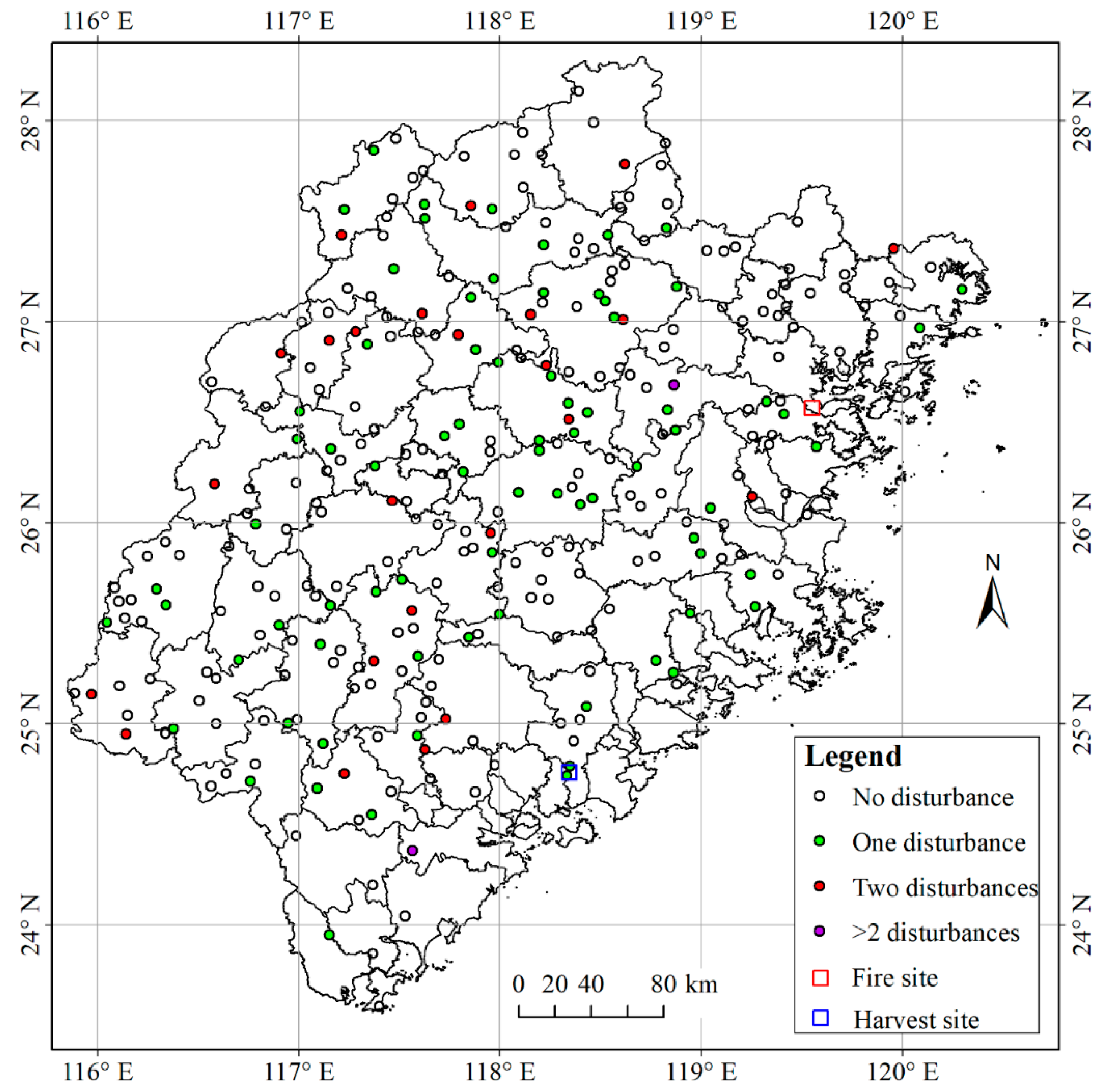
2.1. Study Area and Data

Fujian Province, with the highest forest coverage (66.8%) in China, was selected as the study area to evaluate the importance of adding SWIR bands into forest disturbance monitoring in the subtropical region. Two study sites of forest disturbance for harvest and fire (Figure 1) were selected for qualitative evaluation and to compare the spatial distributions of forest disturbance monitoring with different input and threshold settings. Each site covers an area of 6600 m × 4800 m (220 pixels × 160 pixels). To obtain quantitative assessments, 300 randomly-selected forest reference samples across the Fujian (Figure 1) were well-interpreted to get the forest disturbance types and dates (hereinafter referred to as the reference disturbance dataset). Each sample had the same size as a 30-m spatial resolution Landsat pixel. This reference disturbance dataset provides the forest disturbance type (harvest, fire, and others) and their occurring dates within the year from 1986 to 2021, which were interpreted using multiple data resources including Landsat 5–8, Sentinel-2, Google Earth high-resolution images, and forest inventory data at Fujian. It includes 34.7% of disturbed samples with at least one forest disturbance event, and 65.3% of undisturbed plots without any forest disturbance events during 1986–2021. Of the disturbed samples, 75% of them had only one forest disturbance event during the study period, and the rest had more than one forest disturbance event. The disturbed samples were classified as three major forest disturbance types, including 75% of harvest, 22% of fire, and 3% of others.
The Landsat Collection 2 surface reflectance data from 1986 to 2021 were used to evaluate the values of adding SWIR bands in forest disturbance monitoring. This dataset includes Landsat 5 TM, Landsat 7 ETM+, and Landsat 8 OLI/TIRS data at a 30-m spatial resolution. It has provided the blue band, green band, red band, NIR band, SWIR1, and SWIR2 band surface reflectance since 1986 at Fujian. The band numbers of blue, green, red, NIR, SWIR1, and SWIR2 were shortened as B1, B2, B3, B4, B5, and B6. The QA band was used to screen the clouds, cloud shadows, and some other outliers [22].

2.2. Method

The modified continuous monitoring of land disturbance (COLD) approach [11] was used as the forest disturbance monitoring algorithm for the evaluations. This approach was selected because it can monitor all types of forest disturbances at the sub-annual scale. Another reason was that it did not rely on the availability of training data or complicated inputs heavily because many rules and techniques are based on ecological and biophysical processes [11], making it applicable for large areas and different kinds of environments. In the COLD algorithm, forest disturbance is confirmed by two criteria: one is to measure the differences between the model predictions and satellite observations; the other is to measure the duration of these differences using several consecutive observations [11]. In this study, we modified the COLD by integrating minimum days and minimum consecutive observations to measure the duration of these differences [23,24] for improving the accuracy of forest disturbance monitoring:
min{C(i), C(i + 1),…, C(i + Nm − 1) } ≥ χ2(k, T) and t(i + Nc − 1) − t(i) ≥ Dm
where i: the index of an observation; k: the number of input bands; T: the change threshold; C(i): the change magnitude; χ2(k, T): the threshold derived from the chi-squared distribution; t(i): the date of the observation; Nc: the minimum number of consecutive observations in confirming a forest disturbance; Dm: the minimum days to measure the duration of differences in confirming a forest disturbance. This modification could account for the temporal variability of Landsat time series, and improve the spatial and temporal consistency of forest disturbance monitoring [23,24]. The optimal threshold of Dm using the Landsat time series was set as 80 days according to the study of [23]. The optimal thresholds of Nc (e.g., 4, 5, 6, 7, and 8) and T (e.g., 0.9, 0.95, 0.99, 0.999, and 0.9999) were determined by the sensitivity analysis. 50% of reference disturbance plots (calibrating samples) were randomly selected to calibrate the optimal thresholds for the COLD forest disturbance monitoring with different input band combinations, and the remaining 50% (validating samples) was used to calculate the disturbance monitoring accuracy for each input band combination.
The commission error, omission error, and F1 score are used to indicate the forest disturbance monitoring accuracy [11]. The commission error depicts the error of detected forest disturbance that was not labeled as forest disturbance in the reference disturbance dataset. The omission error depicts the error of forest disturbance in the reference disturbance dataset omitted by the algorithm. The F1 score is the balance of the commission and omission errors [11], and is regarded as the final accuracy.
To evaluate the value of adding a band in forest disturbance monitoring, the modified COLD with different band combinations was applied. It used a harmonic time series model with 3 harmonic items [11] to fit the time series of reflectance at each band, and then integrated the differences between the model predictions and satellite observations of each band using a chi-squared distribution based on the number of input bands, making it applicable for different band combinations. We first tested the modified COLD with all five-band combinations to determine the optimal band combination for forest disturbance monitoring, as the five-band combination was demonstrated to have the highest disturbance monitoring accuracy, even higher than that using all six bands [11]. Then the value of adding one band was evaluated by comparing accuracies with the optimal band combination and optimal band combination minus the specific band. For example, the values of adding the SWIR bands were evaluated by comparing the optimal band combination and corresponding band combinations without the SWIR bands. The value of adding one single SWIR band was also assessed by reducing the SWIR band from the optimal band combination. To shorten the name of band combinations, the band numbers of the blue, green, red, NIR, SWIR1, and SWIR2 bands were reorganized as B1 to B6. For example, R+B+NIR+SWIR1+SWIR2 would be named as B13456.
To evaluate the performance of monitoring specific forest disturbance type (i.e., harvest and fire), the samples with two or more different types of forest disturbance occurring between 1986 and 2021 were removed from calculating the accuracy (F1 score). The not-disturbed samples were also included in the evaluation. The number of randomly selected not-disturbed samples used for evaluating a specific disturbance type was determined by the percentage of disturbing events in the total disturbance events. There were 147 not-disturbed samples (75%) and 65 forest harvest samples used to evaluate forest harvest monitoring, and 43 not-disturbed samples (22%) and 13 forest fire samples used to evaluate forest fire monitoring. Among these samples, 50% were randomly selected to calibrate the optimal thresholds, and the remaining 50% were used to calculate the F1 scores.

3. Results

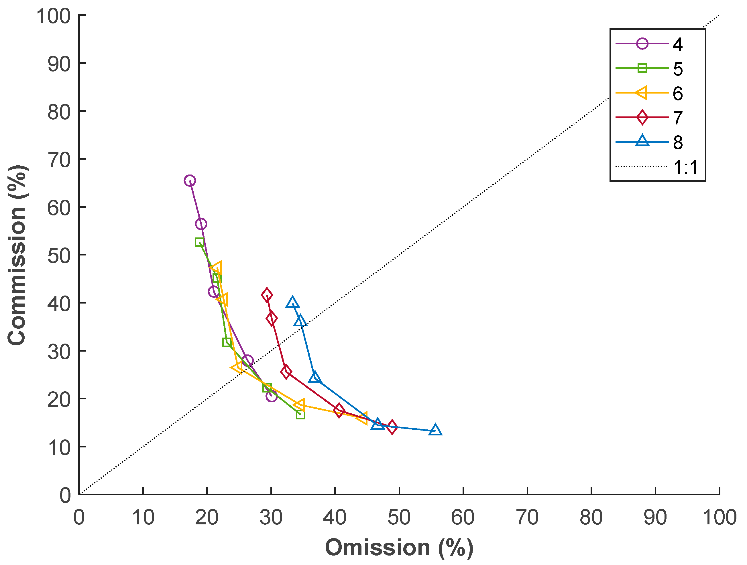
3.1. Accuracy Assessment with Different Band Combinations

Table 1 shows the accuracy of forest disturbance monitoring using different band combinations and the corresponding optimal thresholds of the modified COLD algorithm. The optimal thresholds were derived from the sensitivity analysis using the calibrating samples with a different number of consecutive observations (e.g., 4, 5, 6, 7, and 8) and change thresholds (e.g., 0.9, 0.95, 0.99, 0.999, and 0.9999) used in forest disturbance confirmation. The F1 scores were calculated from the validating samples using the optimal thresholds. Figure 2 presents an example of determining the optimal thresholds in the modified COLD. With the optimal change threshold and the number of consecutive observations being set to 0.99 and 6, respectively, the smallest commission and omission errors were reached in forest disturbance monitoring using the band combination of B13456. Figure 3 shows an example of forest disturbance monitoring by the modified COLD during 1986–2021. The change magnitudes for each disturbance event, which is the delta difference of surface reflectance caused by the disturbance event, exhibited differential variations between different spectral bands.
To evaluate the adding values of the SWIR bands, we conducted forest disturbance monitoring using the four-band combinations and three-band combinations selected based on the two well-performed five-band combinations. As with the comparison using five-band combinations, the four-band combinations with the SWIR2 band obtained overall accuracy ~5% larger than the four-band combinations with the SWIR1 bands. All four-band combinations with one SWIR band achieved overall accuracy 19–26% larger than the four-band combinations without any SWIR bands, i.e., B1234 (44.3%). It is worth noting that the three-band combinations B234 achieved higher accuracy than B1234. All in all, without the two SWIR bands, the overall accuracy of modified COLD forest disturbance monitoring was less than 50%.
The highest accuracy of modified COLD for detecting forest harvest (76.3%) and forest fire (86.6%) was also achieved by the band combinations of B13456, while the optimal change thresholds and the number of consecutive observations in forest disturbance confirmation varied largely. Without the two SWIR bands, the modified COLD could achieve an accuracy of 49.8% in detecting forest harvest and 67.6% in detecting forest fire. These results confirmed the values of adding SWIR bands in the detection of forest harvest and fire.

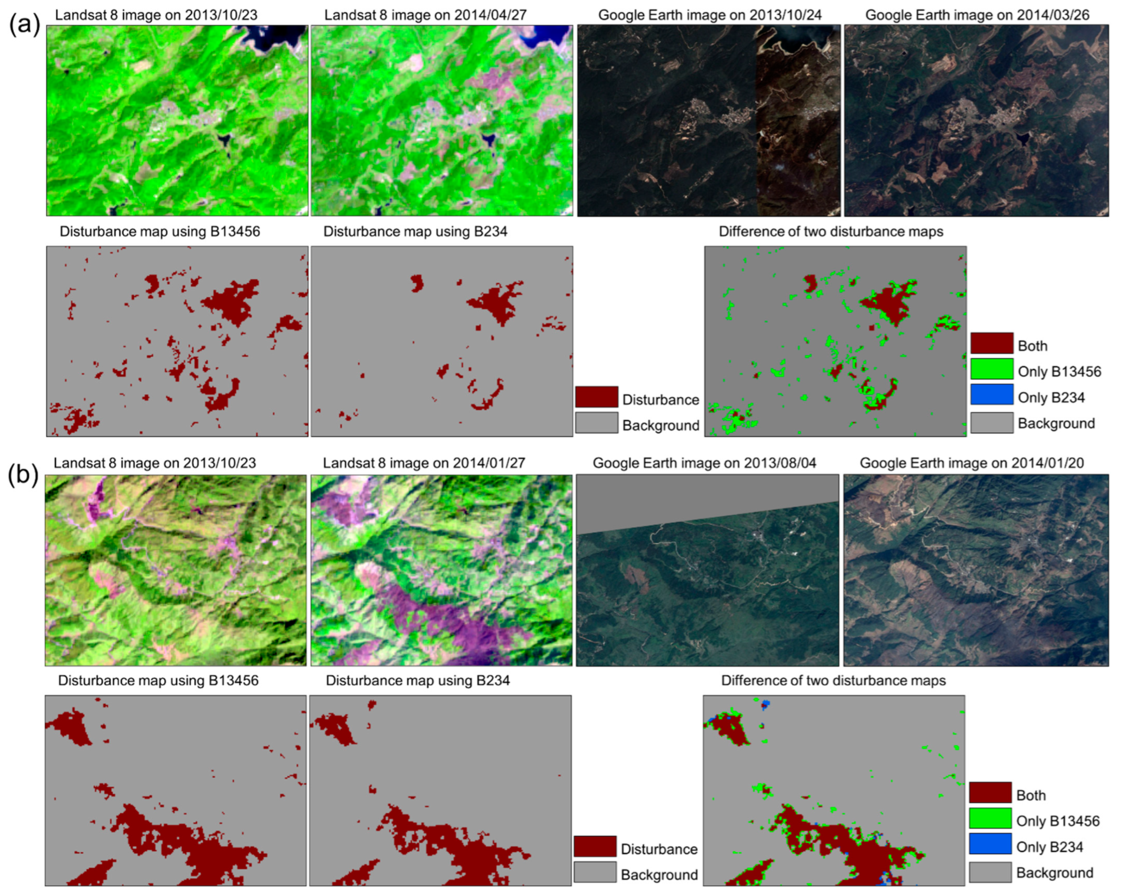
3.2. Forest Harvest and Fire Monitoring Using the Optimal Band Combinations with and without the SWIR Bands

Spatial distributions of monitored forest disturbance using the band combinations with and without the SWIR bands have observing differences. Harvest and fire as the two types of forest disturbance with the largest occurrence areas were selected to demonstrate the values of adding SWIR bands in forest disturbance monitoring. Figure 4 shows typical examples of forest harvest and fire monitoring, respectively, by the modified COLD algorithm with the optimal band combinations with two SWIR bands (B13456) and without any SWIR band (B234). The RGB-composited Landsat 8 images (SWIR1/NIR/R) before and after forest disturbance and the Google earth high-resolution images with the closest imaging time were used as the reference to indicate the performance of COLD forest disturbances monitoring. In Figure 4a, the monitored forest harvests were more approximate to the RGB images using the band combination of B13456 than that using the band combination of B234. Without the SWIR bands, many small forest harvest events and margins for large forest harvest events were omitted. For the reference disturbance samples, there were 89.3% of omitted forest harvest events by the band combination of B234 located at the small forest harvest and the margins of large forest harvest events. Similarly, in Figure 4b, the monitored forest fires were more approximate to the RGB images using the band combination of B13456 than that using the band combination of B234. Without the SWIR bands, some margins of the forest fire were omitted, which occupied 75.7% of omitted forest fire events in the reference disturbance samples.

4. Discussion and Conclusions

This study evaluated the importance of adding SWIR bands in forest disturbance monitoring using the modified COLD algorithm. The absence of SWIR bands decreased the accuracy of forest disturbance monitoring by 19–26%. The highest accuracy using the optimal band combination with SWIR bands was 76.3% for monitoring harvest and 86.6% for monitoring fire, while it decreased to 49.8% in detecting harvest and 67.6% in detecting fire without using any SWIR bands.
The RGB-NIR bands are also critical for forest disturbance monitoring, and many forest disturbances with significant spectral changes could be detected by using the RGB-NIR bands [11]. However, for the water content-related forest disturbance, the SWIR bands have irreplaceable values, because there are more sensitive to the vegetation water content changes than the RGB-NIR bands [14], and the accuracy of forest disturbance monitoring could be significantly improved by integrating the SWIR bands with the RGB-NIR bands.
The randomly selected reference samples may not include all types of forest disturbance in the subtropical region. There were 75% of the harvest and 22% of the fire in the reference samples, while only 3% of other forest disturbance types were included. However, for the purpose of soil carbon modeling, this may not influence the results because harvest and fire are the two critical forest disturbance types that would cause a large amount of carbon emission from soil to the atmosphere [5].
The F1 score was used to indicate the monitoring accuracy, and its calculation only accounted for the samples that were detected as a forest disturbance by the COLD detection or labeled as a forest disturbance in the reference [11]. The samples with no disturbance records in both the reference and COLD detections were excluded from the calculation of the F1 score. This was different from the overall accuracy calculated from the confusion matrix [25], which might be biased by a large number of samples with no disturbance records. For example, if we have 10,000 samples with no disturbance records in both the reference and COLD detections, the overall accuracy calculated from the confusion matrix could be as high as 97%. To avoid these biases, F1 score was chosen to indicate the monitoring accuracy.
In conclusion, this study quantitatively confirmed the importance of adding SWIR bands in forest disturbance monitoring for soil carbon modeling, and provides guidelines for users to select the satellite data with at least one short-wave infrared band to conduct forest disturbance monitoring.

Author Contributions

Conceptualization, methodology, validation, X.L. and Y.C.; formal analysis, S.J., C.W., S.W. and D.R.; writing—original draft preparation, X.L. and Y.C.; writing—review and editing, X.L. and Y.C. All authors have read and agreed to the published version of the manuscript.

Funding

This research was funded by the State Grid Fujian Electric Power Co., Ltd., grant number 52130421000Z.

Institutional Review Board Statement

Not applicable.

Informed Consent Statement

Not applicable.

Acknowledgments

The authors would like to acknowledge the Landsat Collection 2 data downloaded from Google Earth Engine and the TimeSync GEE tools provided by the eMapR Lab for the reference forest disturbance interpretation.

Conflicts of Interest

The authors declare no conflict of interest. The funders had no role in the design of the study; in the collection, analyses, or interpretation of data; in the writing of the manuscript, or in the decision to publish the results.

References

  1. Pellegrini, A.F.A.; Ahlström, A.; Hobbie, S.E.; Reich, P.B.; Nieradzik, L.P.; Staver, A.C.; Scharenbroch, B.C.; Jumpponen, A.; Anderegg, W.R.L.; Randerson, J.T.; et al. Fire Frequency Drives Decadal Changes in Soil Carbon and Nitrogen and Ecosystem Productivity. Nature 2018, 553, 194–198. [Google Scholar] [CrossRef] [PubMed]
  2. Walker, X.J.; Baltzer, J.L.; Cumming, S.G.; Day, N.J.; Ebert, C.; Goetz, S.; Johnstone, J.F.; Potter, S.; Rogers, B.M.; Schuur, E.A.G.; et al. Increasing Wildfires Threaten Historic Carbon Sink of Boreal Forest Soils. Nature 2019, 572, 520–523. [Google Scholar] [CrossRef] [PubMed]
  3. Qin, Y.; Xiao, X.; Wigneron, J.P.; Ciais, P.; Brandt, M.; Fan, L.; Li, X.; Crowell, S.; Wu, X.; Doughty, R.; et al. Carbon Loss from Forest Degradation Exceeds That from Deforestation in the Brazilian Amazon. Nat. Clim. Chang. 2021, 11, 442–448. [Google Scholar] [CrossRef]
  4. Yu, Z.; Zhou, G.; Liu, S.; Sun, P.; Agathokleous, E. Impacts of Forest Management Intensity on Carbon Accumulation of China’s Forest Plantations. For. Ecol. Manage. 2020, 472, 118252. [Google Scholar] [CrossRef]
  5. Bowd, E.J.; Banks, S.C.; Strong, C.L.; Lindenmayer, D.B. Long-Term Impacts of Wildfire and Logging on Forest Soils. Nat. Geosci. 2019, 12, 113–118. [Google Scholar] [CrossRef]
  6. Cohen, W.B.; Healey, S.P.; Yang, Z.; Zhu, Z.; Gorelick, N. Diversity of Algorithm and Spectral Band Inputs Improves Landsat Monitoring of Forest Disturbance. Remote Sens. 2020, 12, 1673. [Google Scholar] [CrossRef]
  7. Tang, X.; Bullock, E.L.; Olofsson, P.; Woodcock, C.E. Can VIIRS Continue the Legacy of MODIS for near Real-Time Monitoring of Tropical Forest Disturbance? Remote Sens. Environ. 2020, 249, 112024. [Google Scholar] [CrossRef]
  8. Hansen, M.C.; Loveland, T.R. A Review of Large Area Monitoring of Land Cover Change Using Landsat Data. Remote Sens. Environ. 2012, 122, 66–74. [Google Scholar] [CrossRef]
  9. Senf, C.; Seidl, R.; Hostert, P. Remote Sensing of Forest Insect Disturbances: Current State and Future Directions. Int. J. Appl. Earth Obs. Geoinf. 2017, 60, 49–60. [Google Scholar] [CrossRef]
  10. Pessôa, A.C.M.; Anderson, L.O.; Carvalho, N.S.; Campanharo, W.A.; Silva Junior, C.H.L.; Rosan, T.M.; Reis, J.B.C.; Pereira, F.R.S.; Assis, M.; Jacon, A.D.; et al. Intercomparison of Burned Area Products and Its Implication for Carbon Emission Estimations in the Amazon. Remote Sens. 2020, 12, 3864. [Google Scholar] [CrossRef]
  11. Zhu, Z.; Zhang, J.; Yang, Z.; Aljaddani, A.H.; Cohen, W.B.; Qiu, S.; Zhou, C. Continuous Monitoring of Land Disturbance Based on Landsat Time Series. Remote Sens. Environ. 2020, 238, 111116. [Google Scholar] [CrossRef]
  12. Boschetti, M.; Stroppiana, D.; Brivio, P.A. Mapping Burned Areas in a Mediterranean Environment Using Soft Integration of Spectral Indices from High-Resolution Satellite Images. Earth Interact. 2010, 14, 1–20. [Google Scholar] [CrossRef]
  13. Zhao, K.; Wulder, M.A.; Hu, T.; Bright, R.; Wu, Q.; Qin, H.; Li, Y.; Toman, E.; Mallick, B.; Zhang, X.; et al. Detecting Change-Point, Trend, and Seasonality in Satellite Time Series Data to Track Abrupt Changes and Nonlinear Dynamics: A Bayesian Ensemble Algorithm. Remote Sens. Environ. 2019, 232, 111181. [Google Scholar] [CrossRef]
  14. Ochtyra, A.; Marcinkowska-Ochtyra, A.; Raczko, E. Threshold- and Trend-Based Vegetation Change Monitoring Algorithm Based on the Inter-Annual Multi-Temporal Normalized Difference Moisture Index Series: A Case Study of the Tatra Mountains. Remote Sens. Environ. 2020, 249, 112026. [Google Scholar] [CrossRef]
  15. Rasheed, F.; Delagrange, S.; Lorenzetti, F. Detection of Plant Water Stress Using Leaf Spectral Responses in Three Poplar Hybrids Prior to the Onset of Physiological Effects. Int. J. Remote Sens. 2020, 41, 5127–5146. [Google Scholar] [CrossRef]
  16. Huang, C.; Goward, S.N.; Masek, J.G.; Thomas, N.; Zhu, Z.; Vogelmann, J.E. An Automated Approach for Reconstructing Recent Forest Disturbance History Using Dense Landsat Time Series Stacks. Remote Sens. Environ. 2010, 114, 183–198. [Google Scholar] [CrossRef]
  17. Kennedy, R.E.; Yang, Z.; Cohen, W.B. Detecting Trends in Forest Disturbance and Recovery Using Yearly Landsat Time Series: 1. LandTrendr—Temporal Segmentation Algorithms. Remote Sens. Environ. 2010, 114, 2897–2910. [Google Scholar] [CrossRef]
  18. Griffiths, P.; Kuemmerle, T.; Baumann, M.; Radeloff, V.C.; Abrudan, I.V.; Lieskovsky, J.; Munteanu, C.; Ostapowicz, K.; Hostert, P. Forest Disturbances, Forest Recovery, and Changes in Forest Types across the Carpathian Ecoregion from 1985 to 2010 Based on Landsat Image Composites. Remote Sens. Environ. 2014, 151, 72–88. [Google Scholar] [CrossRef]
  19. DeVries, B.; Decuyper, M.; Verbesselt, J.; Zeileis, A.; Herold, M.; Joseph, S. Tracking Disturbance-Regrowth Dynamics in Tropical Forests Using Structural Change Detection and Landsat Time Series. Remote Sens. Environ. 2015, 169, 320–334. [Google Scholar] [CrossRef]
  20. Drusch, M.; Del Bello, U.; Carlier, S.; Colin, O.; Fernandez, V.; Gascon, F.; Hoersch, B.; Isola, C.; Laberinti, P.; Martimort, P.; et al. Sentinel-2: ESA’s Optical High-Resolution Mission for GMES Operational Services. Remote Sens. Environ. 2012, 120, 25–36. [Google Scholar] [CrossRef]
  21. Francini, S.; McRoberts, R.E.; Giannetti, F.; Mencucci, M.; Marchetti, M.; Scarascia Mugnozza, G.; Chirici, G. Near-Real Time Forest Change Detection Using PlanetScope Imagery. Eur. J. Remote Sens. 2020, 53, 233–244. [Google Scholar] [CrossRef]
  22. Zhu, Z.; Woodcock, C.E. Automated Cloud, Cloud Shadow, and Snow Detection in Multitemporal Landsat Data: An Algorithm Designed Specifically for Monitoring Land Cover Change. Remote Sens. Environ. 2014, 152, 217–234. [Google Scholar] [CrossRef]
  23. Ye, S.; Rogan, J.; Zhu, Z.; Eastman, J.R. A Near-Real-Time Approach for Monitoring Forest Disturbance Using Landsat Time Series: Stochastic Continuous Change Detection. Remote Sens. Environ. 2021, 252, 112167. [Google Scholar] [CrossRef]
  24. Shang, R.; Zhu, Z.; Zhang, J.; Qiu, S.; Yang, Z.; Li, T.; Yang, X. Near-Real-Time Monitoring of Land Disturbance with Harmonized Landsats 7–8 and Sentinel-2 Data. Remote Sens. Environ. 2022, 278, 113073. [Google Scholar] [CrossRef]
  25. Chen, S.; Woodcock, C.E.; Bullock, E.L.; Arévalo, P.; Torchinava, P.; Peng, S.; Olofsson, P. Monitoring Temperate Forest Degradation on Google Earth Engine Using Landsat Time Series Analysis. Remote Sens. Environ. 2021, 265, 112648. [Google Scholar] [CrossRef]
Figure 1. The study area and distributions of reference forest disturbance samples with different frequencies of disturbance events during 1986–2021.
Sustainability 14 10312 g001
Figure 2. Accuracy (F1 score) comparison of forest disturbance monitoring by the modified COLD algorithm using the band combination of B13456 with different change thresholds (from left to right are 0.9, 0.95, 0.99, 0.999, 0.9999) and numbers of consecutive observations (4, 5, 6, 7, 8) used in disturbance confirmation.
Sustainability 14 10312 g002
Figure 3. Example of forest disturbance monitoring by the modified COLD algorithm during 1986–2021. “break” indicates the occurring date of the forest disturbance. Each color represents a time segment divided by the “breaks”. Each time segment is fitted by a harmonic time series model with 3 harmonic items (shorten as Harmonic Model).
Sustainability 14 10312 g003
Figure 4. Typical examples of forest harvest (a) and fire (b) monitoring by the modified COLD algorithm using the band combination of B13456 and B234. The Landsat 8 images are SWIR1-NIR-R composited RGB images. Google Earth images are derived from Google earth’s high-resolution images. The red color (Both), green color (Only B13456), and blue color (Only B234) in the difference between the two disturbance maps indicate the disturbances that were both detected by B13456 and B234, only detected by B13456, and only detected by B234, respectively.
Sustainability 14 10312 g004
Table 1. The accuracy of forest disturbance monitoring and their optimal thresholds using different band combinations. “B1–B6” indicates the blue, green, red, NIR, SWIR1, and SWIR2 bands. “t” and “c” are the change threshold and the number of consecutive observations used in disturbance confirmation.
BandsAll Forest DisturbanceHarvestFire
tcF1 ScoretcF1 ScoretcF1 Score
B1234560.99673.2%0.99572.8%0.9999479.6%
B124560.99673.0%0.99673.2%0.9999483.0%
B134560.99674.4%0.99676.3%0.9999486.6%
B234560.99673.7%0.99675.7%0.9999486.3%
B123560.99671.0%0.90771.7%0.999575.0%
B123460.99570.9%0.95570.3%0.9999483.1%
B123450.95666.7%0.99569.3%0.999576.0%
B23460.99570.6%0.95572.0%0.9999483.2%
B23450.99664.6%0.99570.2%0.999572.8%
B13460.99571.1%0.9673.2%0.9999482.7%
B13450.95666.2%0.9671.1%0.95571.7%
B12340.9544.3%0.9547.5%0.95464.1%
B2340.9546.7%0.9449.8%0.9467.6%
B1240.9437.0%0.9436.8%0.95462.2%
B1340.9544.5%0.95446.9%0.95461.3%
Publisher’s Note: MDPI stays neutral with regard to jurisdictional claims in published maps and institutional affiliations.

