Integration of Supercritical CO₂ Recompression Brayton Cycle with Organic Rankine/Flash and Kalina Cycles: Thermoeconomic Comparison

Abstract

The use of the organic Rankine cycle (ORC), organic flash cycle (OFC) and Kalina cycle (KC) is proposed to enhance the electricity generated by a supercritical CO₂ recompression Brayton (SCRB) cycle. Novel comparisons of the SCRB/ORC, SCRB/OFC and SCRB/KC integrated plants from thermodynamic, exergoeconomic and sustainability perspectives are performed to choose the most appropriate bottoming cycle for waste heat recovery for the SCRB cycle. For comprehensiveness, the performance of the SCRB/OFC and SCRB/ORC layouts are examined using ten working fluids. The influence of design parameters such as pressure ratio in the supercritical CO₂ (S-CO₂) cycle, pinch point temperature difference in heater and pre-cooler 1, turbine inlet temperature and pressure ratio for the ORC/OFC/Kalina cycles are examined for the main system indicators including the net output power, energy and exergy efficiencies, and unit cost of power production. The order of the exergy efficiencies for the proposed systems from highest to lowest is: SCRB/ORC, SCRB/OFC and SCRB/KC. The minimum unit cost of power production for the SCRB/ORC system is lower than that for the SCRB/KC and SCRB/OFC systems, by 1.97% and 0.75%, respectively. Additionally, the highest exergy efficiencies for the SCRB/OFC and SCRB/ORC systems are achieved when n-nonane and R134a are employed as working fluids for the OFC and ORC, respectively. According to thermodynamic optimization design, the SCRB/ORC, SCRB/OFC and SCRB/KC systems exhibit sustainability indexes of 3.55, 3.47 and 3.39, respectively.

1. Introduction

As the population grows, so typically does demand for energy. Much research has been done on improving power generation technology to meet this demand, often focusing on raising efficiency, lowering cost and reducing environmental impact. Some approaches use renewable energy sources or waste heat. In recent years, combined cycles, in which bottoming cycles utilize waste heat from topping cycles, have received increasing attention and their performance has been analyzed and optimized. Due to its simplicity, compactness, safety and economic advantages, the supercritical carbon dioxide cycle has great potential as a future power generation option. Such plants operate with moderate reactor outlet temperatures (550–750 °C) [1]. Near the critical point, sharp changes in S-CO₂ thermophysical properties occur that can significantly lower the compression work, which can raise the efficiency of the S-CO₂ cycle. This addresses one of the problems with classical Brayton cycles, namely, high compression work. Regarding working fluids for power cycles, among the various options, CO₂ has numerous advantages: non-toxic, low cost, compactness and non-flammability. From an environmental perspective, the ozone depletion potential for CO₂ is zero while its global warming potential is 1 [2]. Since the S-CO₂ cycle operates above the critical point, the fluid remains dense throughout the cycle, reducing the size of turbomachinery [3].

Angelino [4] compared S-CO₂ cycle layouts and concluded that the recompression S-CO₂ cycle attains the highest thermodynamic efficiency. Dostal [5] examined the effect of reheating on the efficiency of the cycle and determined that the use of one reheating step is preferable in the S-CO₂ cycle. Dostal et al. [6] compared the economics of the SCRB cycle and the helium Brayton cycle. They concluded that, by using an S-CO₂ cycle instead of a helium system, a 15% cost saving is achieved. In a second law analysis and optimization study of the S-CO₂ recompression cycle, Sarkar [1] found that, from the viewpoint of exergy analysis, irreversibilities are more significant in heat exchangers than turbo-machinery. He also indicated that the turbine isentropic efficiency affects the system exergy efficiency by 2.5 times more than do the exergy efficiencies of the compressors. Moreover, he showed that pressure drop in the reactor in the SCRB cycle notably affects the cycle second law efficiency. In the S-CO₂ cycle, there is a difference between the fluid specific heats of the cold and hot side flows in recuperators. Therefore, introducing a recompressing compressor as an extra compressor prior to the pre-cooler in the recompression S-CO₂ cycle allows the flow to be split to narrow the gap of specific heat for the low temperature recuperator, leading to a higher thermal efficiency by reducing waste heat.

By employing a suitable bottoming cycle, the performance of the S-CO₂ cycle can be enhanced to use low-grade thermal energy as the heater of the S-CO₂ cycle. To date, numerous cycles have been suggested as bottoming cycles for the S-CO₂ cycle. The rejected heat from the heater of the SCRB can be used in an ORC. Recently, the ORC has attracted much attention for its ability to utilize low temperature heat sources [7]. This, in addition to its simplicity, high reliability and ease of maintenance, can make the ORC appropriate as a bottoming cycle [8]. Besarati et al. [9] proposed three configurations for a S-CO₂ cycle: simple S-CO₂ Brayton cycle, recompression S-CO₂ Brayton cycle and partial cooling S-CO₂ Brayton cycle. Then, they employed an ORC as bottoming cycle for each of the cycles. They found that the integrated recompression S-CO₂ Brayton cycle/ORC has the highest efficiency. Mahmoudi et al. [10] investigated thermodynamically and exergoeconomically a S-CO₂ recompression Brayton cycle with an ORC. They assessed 8 ORC working fluids and found that the best thermodynamic and economic performance is achieved using isobutane and RC318. Specifically, they showed that the second law efficiency is 11.7% higher for the SCRB/ORC cycle than the SCRB cycle, and that the total product unit cost is 5.7% less for the SCRB/ORC cycle than the SCRB cycle. Wang et al. [11] concluded via an exergoeconomic analysis of a SCRB/ORC cycle that its second law efficiency with an isobutane working fluid can exceed 62%. The SCRB/ORC cycle exhibits the lowest total product unit cost when isobutene is utilized as the organic working fluid in the ORC. Song et al. [12] carried out a thermoeconomic analysis for the S-CO₂ cycle combined with ORC for geothermal power generation. They revealed that the geothermal combined system with the ORC utilizing waste heat from the S-CO₂ cycle provides 2940 kW of net power output, which is 45% more than that of the S-CO₂ cycle. The thermoeconomic analysis showed that the specific cost of the combined cycle is 2880 $/kW, 22% less than for the S-CO₂ cycle. In another study, Song et al. [13] studied an S-CO₂ cycle combined with an ORC for waste heat recovery for an internal combustion engine (ICE). They determined the net power output to be 215 kW for the combined cycle, which is 58% greater than that of the standalone S-CO₂ cycle, and that the specific investment cost related to the integrated cycle is 4% higher than that of S-CO₂ cycle_. Gutierrez et al. [14] also analyzed a S-CO₂ cycle integrated with an ORC thermodynamically and exergoeconomically, and concluded that cyclohexane is the best choice as the ORC working fluid and that the specific investment for the system is 2310 $/kW.

Habibi et al. [15] considered 13 different working fluids in a supercritical Brayton cycle integrated with an ORC, and found the highest net power output and exergy efficiency, at 177,300 kW and 21.2%, respectively, when helium is used in a supercritical Brayton cycle. Wang et al. [16] compared thirty potential working fluids to be used in an ORC utilizing waste heat from an S-CO₂ cycle, based on achieving optimal mass flow rate, supercritical pressure and superheated temperature. The supercritical temperatures of all thirty working fluids were varied from 50 to 225 °C. In a study of the S-CO₂ cycle combined with an ORC dual loop for waste heat recovery for a diesel engine, Liang et al. [17] obtained the maximum system power output as 40.9 MW, which is 6.7% more than that of the dual-fuel engine. In another paper, Chen et al. [18] performed a thermo-environmental analysis on the combined S-CO₂/ORC system. For enhancing the efficiency of the S-CO₂ cycle combined with an ORC, both subcritical and transcritical ORC systems were considered. The results demonstrated that, compared to the original waste-to-energy plant, the turbine output power and waste-to-energy efficiency for the S-CO₂/subcritical organic Rankine cycle system are increased by $9.50\times {10}^6$ W and 59.4%, respectively, while the power generation and waste-to-energy efficiency of S-CO₂/transcritical organic Rankine cycle system are raised by $10.2\times {10}^6$ W and 63.7%, respectively. Moreover, they have found that, from the viewpoints of first law efficiency and environmental performance, the combined cycle comprised of the S-CO₂/transcritical organic Rankine cycle is more efficient than the S-CO₂/subcritical organic Rankine cycle. They also analyzed the system from an environmental perspective. The sustainable index of the S-CO₂ cycle/subcritical ORC is 1.54, while it is 1.57 for the S-CO₂ cycle/transcritical ORC. Wang et al. [19] contrasted three cycles for a nuclear hydrogen production (NHP) system: steam Rankine cycle (SRC), S-CO₂ and combined S-CO₂/ORC. They showed that, when the inlet temperatures of the reactor in the S-CO₂ cycle are 400 °C and 587 °C, the first law efficiency of the S-CO₂ cycle varies from 27.5% to 31.0% and 27.5% to 36.5%, respectively. Ma et al. [20] utilized waste heat of the engine exhaust gas by combining the supercritical CO₂ Brayton cycle and transcritical ORC, and analyzed the cycle thermodynamically and economically. The greatest exergy destruction was observed to occur in the heater. In addition, they found that the highest exergy efficiency of the system is 54.63% and the lowest levelized cost of energy is 36.95 USD/MWh. Javanshir et al. [21] compared two combined cycles: Brayton/ORC and steam Rankine/ORC. They found that the best working fluids for the Brayton cycle are air and CO₂, and that the highest efficiency is achieved when isobutane, R11 and ethanol are employed as working fluids for the ORC.

Another option as a bottoming cycle for waste heat recovery for the SCRB cycle is the OFC. Wu et al. [22] compared two bottoming cycles (SCRB/OFC and SCRB/ORC) for waste heat recovery from a S-CO₂ cycle thermodynamically and exergoeconomically. They considered seven working fluids in the combined cycles and found that the second law efficiency of the SCRB/OFC cycle is 6.57% greater than that of the SCRB cycle. The total product unit cost for the SCRB/OFC cycle was determined to be 3.75% lower than that of the SCRB cycle. They concluded that the maximum second law efficiency and minimum total product unit cost of the SCRB/OFC cycle are attained using n-nonane as the working fluid.

Another possible cycle that can be used as a bottoming cycle for a S-CO₂ cycle is the Kalina cycle. Since the Kalina cycle boiling/condensing process is at a temperature that is not constant, irreversibilities in the evaporator and condenser are reduced, increasing the second law efficiency [23]. Mahmoudi et al. [24] assessed a SCRB/KC cycle exergoeconomically and found that the exergy efficiency of the SCRB/KC cycle exceeds that of the SCRB cycle by 10% and the total product unit cost for the SCRB/KC cycle is 4.9% less than that of the SCRB cycle. Li et al. [25] also compared SCRB/KC and SCRB cycles and determined the second law efficiency of the SCRB/KC cycle is 8.0% higher than that of the SCRB cycle; however, the total product unit cost for the SCRB/KC cycle is 5.5% lower than that of the SCRB cycle. In a study of a supercritical CO₂ Brayton cycle combined with a Kalina cycle, Feng et al. [26] showed that the average annual fuel consumption is decreased by 16.6% by using this combined system compared to marine power generation auxiliary engines.

Clearly, a good deal of attention has been dedicated to finding beneficial ways to employ the waste heat of a SCRB cycle and numerous bottoming cycles have been proposed. In the present paper, three different bottoming cycles are assessed and compared: OFC, ORC and KC. The novelty of this work lies in optimizing the performance of the SCRB/ORC and SCRB/OFC integrated power systems, regarding selection of the best working fluid for the ORC/OFC bottoming cycles. The performances of the aforementioned systems are then compared with the that of the SCRB/Kalina integrated plant, from thermodynamic, economic and sustainability viewpoints. The objective is to improve understanding of the systems, so as to allow decision makers to choose the best bottoming cycle among ORC/OFC/Kalina cycles for waste heat recovery applications for the S-CO₂ cycle.

2. System Description and Assumptions

The proposed SCRB/OFC cycle is illustrated in Figure 1. In this combined cycle, the OFC utilizes waste heat of the SCRB cycle in a heater. In the SCRB cycle, the CO₂ (state 5), after receiving heat from the reactor, expands and produces work in the S-CO₂ turbine (ST). Part of the expanded stream (state 6) transfers heat to the fluid at state 2 and the other part transfers heat to the fluid at state 3 in the low temperature recuperator (LTR) and high temperature recuperator (HTR), respectively. Then, the CO₂ stream splits into the CO₂ stream 8a entering the heater with a high mass flow rate and the CO₂ stream 8b entering the recompression compressor (RC) with a low mass flow rate. In the heater, CO₂ stream 8a transfers heat to the organic working fluid in the OFC; the stream is then cooled in the pre-cooler. Next, the stream (state 1) is compressed in the main compressor (MC). The compressed CO₂ (state 2) in the MC is mixed with the compressed stream in the RC after being heated in the LTR. The mixture enters the reactor used in the SCRB cycle after absorbing heat in the HTR. In the OFC, the saturated liquid organic working fluid (state 12) is conveyed to the heater where it absorbs heat from hot CO₂. This stream (state 13) is a saturated liquid at higher temperature. The hot stream (state 14) expands in valve 1. The stream at the inlet of the flash separator (Fs) (state 15) is separated to a saturated vapor (state 16) and a saturated liquid (state 18). The stream at state 16 expands and produces work in the turbine, while the stream at state 18 expands in valve 2 to mix with the turbine outlet flow (state 17) in the mixer. Finally, the mixture stream is condensed in the condenser to a saturated liquid.

A schematic for the proposed SCRB/ORC is shown in Figure 2. In this cycle, the ORC utilizes waste heat of the SCRB cycle instead of the OFC. The system description of the SCRB cycle is as above. In the ORC, the saturated liquid (state 12) organic working fluid is pumped to a higher pressure at state 13. The pressurized stream absorbs heat from hot CO₂ in the heater. The hot organic working fluid (state 14) expands and generates work in the turbine. The turbine outlet flow (state 15) becomes a saturated liquid in the condenser.

Figure 3 illustrates the SCRB/KC cycle. In this combination, the KC is the bottoming cycle. The KC utilizes waste heat of the SCRB cycle in the superheater (sup) and pre-cooler 1. The schematic of the SCRB cycle combined with the KC is somewhat different from above two descriptions. In the SCRB cycle, the outlet stream of the LTR is split into two. One part enters the superheater and the other the RC. The superheater outlet flow releases heat to the ammonia-water in pre-cooler 1. Then, this stream is cooled in pre-cooler 2 and compressed in the MC. The SCRB cycle in the SCRB/KC cycle operates just like the SCRB/OFC cycle. In the KC, the saturated ammonia-water liquid (state 20) is passed to the Kalina cycle low temperature recuperator (KCLTR). After absorbing heat in KCLTR, stream (state 22) enters the Kalina cycle high temperature recuperator (KCHTR). The outlet flow of the KCHTR (state 23) enters pre-cooler 1 to be heated by hot CO_2. Then, the stream is separated to saturated liquid (state 13) and saturated vapor (state 12) parts. The saturated vapor absorbs heat in the superheater, while the saturated liquid is cooled in the KCHTR and expands through the valve. The outlet flow of the superheater (state 14) expands and generates work in the turbine and mixes with the outlet flow of the expansion valve in the mixer. The mixture (state 18) is cooled in the KCLTR and then condensed to a saturated liquid in the condenser.

One of the most significant factors that directly affects the overall thermodynamic and economic performance is the working fluid selection. Various factors are considered during the selection such as safety and environmental impact. The latter factors are include ozone depletion potential (ODP) and global warming potential (GWP) [27]. Lower values of ODP and GWP are preferable when selecting working fluids [28]. Other factors are also important in selecting the working fluid:

• Use of a dry working fluid is suggested for preventing turbine blade erosion [29]. This characteristic suggests having a superheated outflow from the turbine.
• A working fluid with high critical temperature and low critical pressure is recommended. A low critical pressure provides the opportunity for a superheated outflow from the turbine with low heat input.

Based on the above factors, ten working fluids are considered for the SCRB/ORC and SCRB/OFC in this study. Thermophysical and environmental properties of these ten working fluids are summarized in

Table 1. Thermophysical and environmental properties of ten working fluidss utilized in SCRB/OFC and SCRB/ORC cycles.

Working Fluid	Thermophysical Properties		Environmental Properties
	Critical Temperature (K)	Critical Pressure (kPa)	ODP	GWP (100 Year) (Relative to CO2)
R245fa	427.2 [30]	3640 [30]	0 [29]	950 [29]
n-Pentane	469.7 [30]	3370 [30]	0 [31]	0 [31]
n-Hexane	507.82 [30]	3034 [30]	0 [31]	0 [31]
n-Heptane	540.13 [30]	2736 [30]	0 [32]	3 [32]
n-Octane	569.32 [30]	2497 [30]
n-Nonane	594.55 [30]	2281 [30]
R123	456.83 [29]	3662 [29]	0.012 [29]	120 [29]
R142b	479.96 [29]	4460 [29]	0.086 [29]	700 [29]
R134a	374.21 [29]	4056 [29]	0 [29]	1300 [29]
Isobutane	425.12 [29]	3796 [29]	0.12 [29]	725 [29]

.

To simplify the modeling and simulation, the following assumptions are used:

(1)

The systems operate under steady state conditions.

(2)

Pressure drops in all heat exchangers and pipelines are negligible.

(3)

Turbines, pumps and compressors have constant isentropic efficiencies.

(4)

Changes in kinetic and potential energies are negligible.

(5)

The cooling water enters the pre-cooler and condenser at ambient temperature and pressure.

(6)

At the heater and condenser outlets, the working fluid is in a saturated liquid state [33].

(7)

The HTR and LTR have constant effectiveness values.

(8)

At the outlets of the separator and condenser, the ammonia-water mixture is in a saturated liquid state.

3. Modeling and Analysis

Using the input data in

Table 2. Input data used for thermodynamic and economic modeling systems.

System	Parameter	Value Reference
S-CO2 Brayton cycle	Cycle minimum temperature (°C)	32 [11,34]
	Cycle maximum temperature (°C)	550 [11,34]
	Main compressor inlet pressure (bar)	74 [11,34]
	Compressor pressure ratio, Prc	2.2–4.2 [11,34]
	LTR and HTR effectiveness, ${\epsilon }_{LTR}$ and ${\epsilon }_{HTR}$ (%)	86 [1,5,35]
	S-CO2 turbine isentropic efficiency, ${\eta }_{ST}$ (%)	90 [1,5,35]
	Main compressor isentropic efficiency, ${\eta }_{MC}$ (%)	85 [1,5,35]
	Recompression compressor isentropic efficiency, ${\eta }_{RC}$ (%)	85 [1,5,35]
	Pinch point temperature difference in Heater, $\Delta T_{He}$ (K)	8–16 [22]
	Pinch point temperature difference in Pre-cooler 1, $\Delta T_{\mathrm{Pr}e1}$ (K)	8–16 [22]
	Heat provided by Reactor, ${\dot{Q}}_R$ (MW)	600 [1,5,35]
Bottoming cycle Organic flash cycle	Reactor core temperature, $T_R$ (°C) Turbine isentropic efficiency, ${\eta }_T$ (%) Pump isentropic efficiency, ${\eta }_P$ (%) Flash separator inlet temperature, $T_{15}$ (°C) Pinch point temperature difference in Condenser, $\Delta T_{Cond}$ (K)	800 [1,5,35] 80 [36] 80 [36] 80 [36] 10 [22]
Organic Rankine cycle	Turbine inlet temperature, $T_{14}$ (°C) Pinch point temperature difference in Condenser, $\Delta T_{Cond}$ (K) Degree of superheat, $\Delta T_{Sup}$ (K)	90 [11] 10 [22] 0 [11]
Kalina cycle	Separator inlet temperature, $T_{11}$ (°C) Ammonia concentration in ammonia-water mixture leaving the condenser, X20 (%) Pump pressure ratio, Prpump Minimum temperature difference in superheater, ${{\displaystyle \Delta T}}_{\sup }$ (K) Standard chemical exergy of ammonia, $e_{ch,NH3}^0(\mathrm{J}/\mathrm{mol})$ Standard chemical exergy of water, $e_{ch,H2O}^0(\mathrm{J}/\mathrm{mol})$	79.85 [24] 95 [24] 2.55–3.65 [24] 1 [11] 337,900 [37] 900 [37]
Economic data	Interest rate, $i_r$ Number of operation year, n Annual plant operation hours, $\tau$ Maintenance factor, $\gamma$ Fuel cost, ${{\displaystyle c}}_{fuel}$($/MWh)	0.12 [10] 20 [10] 8000 [10] 0.06 [10] 7.4 [38]
Ambient condition	Ambient temperature, T0 (k)	298.15
	Ambient pressure, P0 (bar)	1

, the proposed systems are simulated by Engineering Equation Solver (EES). The thermodynamic and economic principles applied to model the systems are listed and described in subsequent sections.

3.1. Thermodynamic Analysis

Considering assumptions 1 and 4, mass, energy and exergy balance equations respectively for each system component as a control volume (CV) can be written as follows:

$${\displaystyle \sum {{\displaystyle \dot{m}}}_{in}=}{\displaystyle \sum {{\displaystyle \dot{m}}}_{out}}$$

(1)

$${\displaystyle \sum \dot{Q}+}{\displaystyle \sum {\dot{m}}_{in}{h}_{in}=}{\displaystyle \sum {\dot{m}}_{out}{h}_{out}}+\dot{W}$$

(2)

$${\dot{E}}_Q+{\displaystyle \sum {\dot{E}}_{in}=}{\displaystyle \sum {\dot{E}}_{out}}+\dot{W}+{\dot{E}}_D$$

(3)

where $\dot{Q}$, $\dot{W}$ and $\dot{E}$ denote heat transfer rate, work rate and exergy flow rate entering or exiting the CV and the subscripts in, out and D represent the CV inlet and outlet, and destruction. The overall exergy rate of a stream is the aggregate of its physical and chemical exergy rates, defined as follows [22]:

$${{\displaystyle \dot{E}}}_{}={{\displaystyle \dot{E}}}_{ph}+{{\displaystyle \dot{E}}}_{ch}$$

(4)

The physical exergy is calculated by [39]:

$${\dot{E}}_{ph}=\dot{m}((h-h_0)-T_0(s-s_0))$$

(5)

Since the supercritical CO₂ and organic fluids used in the corresponding cycles are considered to be pure substances and their structures do not change during the cycle processes, their chemical exergies at different states are the same. Therefore, the exergy destruction rate of components in the mentioned cycles is affected just by the thermophysical exergy rates. In this regard, there is no necessity to evaluate the chemical exergy for analyzing the cycles. However, the ammonia concentration is continuously changing during the various processes in the Kalina cycle. Thus, it is required to define chemical exergy for the ammonia-water working fluid, and this is done as follows [37]:

$${{\displaystyle \dot{E}}}_{ch}={{\displaystyle \dot{m}}}_{}((\frac{X}{{{\displaystyle M}}_{NH3}})e_{ch,NH3}^0+(\frac{X}{{{\displaystyle M}}_{H2O}})e_{ch,H2O}^0)$$

(6)

where X is the ammonia concentration in the ammonia-water mixture, and $e_{ch,NH3}^0$ and $e_{ch,H2O}^0$ are the standard chemical exergies of ammonia and water, respectively [37].

The first law efficiency for the combined cycles is defined as follows:

$${\eta }_{th}=\frac{{\dot{W}}_{net,tot}}{{\dot{Q}}_R}$$

(7)

where ${\dot{W}}_{net,tot}$ is the total net output power and ${\dot{Q}}_R$ is the heat provided by the reactor. Another important thermodynamic indicator is the second law efficiency, defined as follows:

$${\eta }_{ex}=\frac{{\dot{W}}_{net,tot}}{{\dot{E}}_R}$$

(8)

where ${\dot{E}}_R$ is the exergy provided by the reactor.

3.2. Thermoeconomic Analysis

In order to calculate the product unit cost of the system and minimize it, a thermoeconomic analysis is applied, based on the specific exergy costing (SPECO) method [24]. This method includes the following three main steps: (1) obtaining exergy values for each state of the system, (2) determining the fuels and products for each component and (3) implementing cost balances and auxiliary equations and solving the resulting system equations [40].

The cost rate balance equation can be written as [39]:

$${\displaystyle \sum {{\displaystyle \dot{C}}}_{out}}+{{\displaystyle \dot{C}}}_w={\displaystyle \sum {{\displaystyle \dot{C}}}_{in}}+{{\displaystyle \dot{C}}}_q+{{\displaystyle \dot{Z}}}_k$$

(9)

$$\dot{C}=c\dot{E}$$

(10)

where ${{\displaystyle \dot{C}}}_{in}$, ${{\displaystyle \dot{C}}}_{out}$ and ${{\displaystyle \dot{Z}}}_k$ denote the cost rates associated with fuel, product and the sum of the capital investment and operating and maintenance costs of each system component, respectively. The last term can be defined as follows:

$${\dot{Z}}_k={\dot{Z}}_k^{CI}+{\dot{Z}}_k^{OM}$$

(11)

where ${\dot{Z}}_k^{CI}$ and ${\dot{Z}}_k^{OM}$ are the annual capital investment and operating and maintenance cost rates, respectively. For each component, the above terms are given by [39]:

$${\dot{Z}}_k^{CI}=(\frac{CRF}{\tau })Z_k$$

(12)

$${\dot{Z}}_k^{OM}=(\frac{\gamma }{\tau })Z_k$$

(13)

where CRF is capital recovery factor and can be calculated by:

$$CRF=\frac{{{\displaystyle i}}_r{(1+{{\displaystyle i}}_r)}^n}{{(1+{{\displaystyle i}}_r)}^n-1}$$

(14)

Here, $\tau$, $\gamma$, $n$ and ${{\displaystyle i}}_r$ denote annual plant operation hours, maintenance factor, number of years of economic life and interest rate, respectively, and values for these parameters are given in Table 2. In addition, the cost functions for each component are given in

Table A1. Cost functions and CEPCI0 for each component of the systems.

Component	Cost Function	Reference Year	CEPCI0	Reference
Reactor	$Z_R=c_{in}{\dot{Q}}_R,c_{in}=283\$/K{W}_{th}$	2003	402.3	[38]
S-CO2 turbine	$Z_{ST}=479.34\times {\dot{m}}_{in}\times (\frac{1}{0.93-{\eta }_{ST}})\times Ln({\mathrm{Pr}}_c)\times (1+\exp (0.036\times T_{in}-54.4))$	1994	368.1	[39]
Compressors	$Z_{MC\&RC}=71.1\times {\dot{m}}_{in}\times (\frac{1}{0.92-{\eta }_c})\times {\mathrm{Pr}}_c\times Ln({\mathrm{Pr}}_c)$	1994	368.1	[39]
HTR, LTR, Pre-cooler 1, Heater and Superheater	$Z_k=2681\times A_k{}^{0.59}$	1986	318.4	[50]
KCLTR, KCHTR, Condenser, Pre-cooler, Pre-cooler 2	$Z_k=2143\times {{{\displaystyle A}}_k}^{0.514}$	1986	318.4	[50]
Turbine	$Z_T=4405\times {({\dot{W}}_T)}^{0.7}$	2005	468.2	[51]
Pump	$Z_P=1120\times {({\dot{W}}_P)}^{0.8}$	2005	468.2	[51]

.

All cost data in the original year are converted to 2019 using the chemical engineering plant cost index (CEPCI), as follows [41]:

$${{\displaystyle \dot{Z}}}_{k,2019}={{\displaystyle \dot{Z}}}_k(\frac{CEPC{I}_{2019}}{CEPC{I}_0})$$

(15)

where $CEPC{I}_{2019}$ is 603.1 [42] and $CEPC{I}_0$ denotes the chemical engineering plant cost index of original year for each component, as summarized in Table A1.

Finally, the total product unit cost of the system can be written as follows [12]:

$${{\displaystyle c}}_{P,tot}=\frac{{\displaystyle \sum _{i=1}^{nk}{{\displaystyle \dot{Z}}}_k+{{\displaystyle \dot{C}}}_{fuel}}}{{\displaystyle {\sum }_{i=1}^{np}{{\displaystyle \dot{E}}}_{Pi}}}$$

(16)

where ${{\displaystyle \dot{C}}}_{fuel}$ denotes the cost rate associated with fuel and ${\displaystyle {\sum }_{i=1}^{np}{{\displaystyle \dot{E}}}_{Pi}}$ the exergy rate of system products, i.e., the total net power produced by each combined cycle. This indicator is an important parameter that gives researchers much information about the economic performance of the system and it helps compare systems economically. Note that systems operate at their best economic performances when this indicator is a minimum.

3.3. Sustainability Analysis

Sustainability analysis is employed to describe and illustrate the relationship between exergy and ecological impact [43]. To do this, the sustainability index is utilized, which is defined as [44]:

$$SI=\frac{1}{D_p}$$

(17)

Here, $D_p$ is the depletion number, which can be written as [45]:

$$D_p=\frac{{\dot{E}}_D}{{\dot{E}}_R}$$

(18)

The sustainability index suggests not only utilizing renewable energies, but also employing non-renewable energy sources. The sustainability index also illustrates that reducing irreversibilities lowers ecological impacts, which is preferable.

The fuel utilized in this paper is TRISO coated particle fuel, which stands for TRI-structural isotropic particle fuel. Each TRISO particle is made up a uranium, carbon and oxygen fuel kernel [46]. Energy, exergy and cost rate balance equations of each component for SCRB/OFC, SCRB/ORC and SCRB/KC are listed in

Table 3. Energy, exergy and cost rate balances and auxiliary equations for each component of SCRB/OFC cycle.

Component	Energy Balance	Exergy Balance	Cost Rate Balance and Ancillary Equation
Main compressor	${\dot{m}}_1{h}_1+{\dot{W}}_{MC}={\dot{m}}_2{h}_2$ ${\eta }_{MC}=(h_{2s}-h_1)/(h_2-h_1)$	${\dot{E}}_1+{\dot{W}}_{MC}={\dot{E}}_2+{\dot{E}}_{D,MC}$	${\dot{C}}_1+{\dot{C}}_{MC}+{\dot{Z}}_{MC}={\dot{C}}_2$ $c_{MC}=c_{ST}$
Recompression compressor	${\dot{m}}_{8b}{h}_{8b}+{\dot{W}}_{RC}={\dot{m}}_{3b}{h}_{3b}$ ${\eta }_{RC}=(h_{3s}-h_8)/(h_3-h_8)$	${\dot{E}}_{8b}+{\dot{W}}_{RC}={\dot{E}}_{3b}+{\dot{E}}_{D,RC}$	${\dot{C}}_{8b}+{\dot{C}}_{RC}+{\dot{Z}}_{RC}={\dot{C}}_{3b}$ $c_{RC}=c_{ST},c_{8b}=x{c}_8$
S-CO2 turbine	${\dot{m}}_5{h}_5={\dot{W}}_{ST}+{\dot{m}}_6{h}_6$ ${\eta }_{ST}=(h_5-h_6)/(h_5-h_{6s})$	${\dot{E}}_5={\dot{W}}_{ST}+{\dot{E}}_6+{\dot{E}}_{D,ST}$	${\dot{C}}_5+{\dot{Z}}_{ST}={\dot{C}}_6+{\dot{C}}_{ST}$ $c_5=c_6$
Reactor	${\dot{m}}_4{h}_4+{\dot{Q}}_R={\dot{m}}_5{h}_5$	${\dot{E}}_4+{\dot{Q}}_R(1-\frac{T_0}{T_R})={\dot{E}}_5+{\dot{E}}_{D,R}$	${\dot{C}}_4+{\dot{C}}_{fuel}+{\dot{Z}}_R={\dot{C}}_5$
HTR	${\dot{m}}_3{h}_3+{\dot{m}}_6{h}_6={\dot{m}}_4{h}_4+{\dot{m}}_7{h}_7$ ${{\displaystyle \epsilon }}_{HTR}=\frac{{{\displaystyle T}}_6-{{\displaystyle T}}_7}{{{\displaystyle T}}_6-{{\displaystyle T}}_3}$	${\dot{E}}_3+{\dot{E}}_6={\dot{E}}_4+{\dot{E}}_7+{\dot{E}}_{D,HTR}$	${\dot{C}}_3+{\dot{C}}_6+{\dot{Z}}_{HTR}={\dot{C}}_4+{\dot{C}}_7$ $c_7=c_6,{\dot{C}}_3={\dot{C}}_{3a}+{\dot{C}}_{3b}$
LTR	${\dot{m}}_2{h}_2+{\dot{m}}_7{h}_7={\dot{m}}_{3a}{h}_{3a}+{\dot{m}}_8{h}_8$ ${{\displaystyle \epsilon }}_{LTR}=\frac{{{\displaystyle T}}_7-{{\displaystyle T}}_8}{{{\displaystyle T}}_7-{{\displaystyle T}}_2}$	${\dot{E}}_2+{\dot{E}}_7={\dot{E}}_{3a}+{\dot{E}}_8+{\dot{E}}_{D,LTR}$	${\dot{C}}_2+{\dot{C}}_7+{\dot{Z}}_{LTR}={\dot{C}}_{3a}+{\dot{C}}_8$ $c_7=c_8$
Pre-cooler	${\dot{m}}_9{h}_9-{\dot{m}}_1{h}_1={\dot{m}}_{11}{h}_{11}-{\dot{m}}_{10}{h}_{10}$	${\dot{E}}_9+{\dot{E}}_{10}={\dot{E}}_1+{\dot{E}}_{11}+{\dot{E}}_{D,pre}$ ${\dot{E}}_{11}={\dot{E}}_{10}+{\dot{E}}_{L,pre}$	${\dot{C}}_9+{\dot{C}}_{10}+{\dot{Z}}_{\mathrm{Pr}e}={\dot{C}}_1+{\dot{C}}_{11}$ $c_1=c_9,{\dot{C}}_{10}=0$
Heater	${\dot{m}}_9{h}_9+{\dot{m}}_{14}{h}_{14}={\dot{m}}_{8a}{h}_{8a}+{\dot{m}}_{13}{h}_{13}$	${\dot{E}}_{8a}+{\dot{E}}_{13}={\dot{E}}_9+{\dot{E}}_{14}+{\dot{E}}_{D,Heater}$	${\dot{C}}_{8a}+{\dot{C}}_{13}+{\dot{Z}}_{Heater}={\dot{C}}_9+{\dot{C}}_{14}$ $c_{8a}=c_9,{\dot{C}}_{8a}=(1-x){\dot{C}}_8$
Valve 1	${\dot{m}}_{14}{h}_{14}={\dot{m}}_{15}{h}_{15}$	${\dot{E}}_{14}={\dot{E}}_{15}+{\dot{E}}_{D,V1}$	${\dot{C}}_{14}+{\dot{Z}}_{V1}={\dot{C}}_{15}$
Valve 2	${\dot{m}}_{18}{h}_{18}={\dot{m}}_{19}{h}_{19}$	${\dot{E}}_{18}={\dot{E}}_{19}+{\dot{E}}_{D,V2}$	${\dot{C}}_{18}+{\dot{Z}}_{V2}={\dot{C}}_{19}$
Flash separator	${\dot{m}}_{15}{h}_{15}={\dot{m}}_{16}{h}_{16}+{\dot{m}}_{18}{h}_{18}$	${\dot{E}}_{15}={\dot{E}}_{16}+{\dot{E}}_{18}+{\dot{E}}_{D,Flash}$	${\dot{C}}_{15}+{\dot{Z}}_{Flash}={\dot{C}}_{16}+{\dot{C}}_{18}$ $\frac{({\dot{C}}_{16}-{\dot{C}}_{15})}{({\dot{E}}_{16}-{\dot{E}}_{15})}=\frac{({\dot{C}}_{18}-{\dot{C}}_{15})}{({\dot{E}}_{18}-{\dot{E}}_{15})}$
Mixer	${\dot{m}}_{17}{h}_{17}+{\dot{m}}_{19}{h}_{19}={\dot{m}}_{20}{h}_{20}$	${\dot{E}}_{17}+{\dot{E}}_{19}={\dot{E}}_{20}+{\dot{E}}_{D,Mixer}$	${\dot{C}}_{17}+{\dot{C}}_{19}+{\dot{Z}}_{Mixer}={\dot{C}}_{20}$
Pump	${\dot{m}}_{12}{h}_{12}+{\dot{W}}_{Pump}={\dot{m}}_{13}{h}_{13}$ ${\eta }_P=(h_{13s}-h_{12})/(h_{13}-h_{12})$	${\dot{E}}_{12}+{\dot{W}}_{Pump}={\dot{E}}_{13}+{\dot{E}}_{D,Pump}$	${\dot{C}}_{12}+{\dot{C}}_{Pump}+{\dot{Z}}_{Pump}={\dot{C}}_{13}$ $c_{Pump}=c_{Turbine}$
Turbine	${\dot{m}}_{16}{h}_{16}={\dot{W}}_{Turbine}+{\dot{m}}_{17}{h}_{17}$ ${\eta }_T=(h_{16}-h_{17})/(h_{16}-h_{17s})$	${\dot{E}}_{16}={\dot{W}}_{Turbine}+{\dot{E}}_{17}+{\dot{E}}_{D,Turbine}$	${\dot{C}}_{16}+{\dot{Z}}_{Turbine}={\dot{C}}_{17}+{\dot{C}}_{Turbine}$ $c_{16}=c_{17}$
Condenser	${\dot{m}}_{20}{h}_{20}+{\dot{m}}_{21}{h}_{21}={\dot{m}}_{12}{h}_{12}+{\dot{m}}_{22}{h}_{22}$	${\dot{E}}_{20}+{\dot{E}}_{21}={\dot{E}}_{12}+{\dot{E}}_{22}+{\dot{E}}_{D,Cond}$ ${\dot{E}}_{22}={\dot{E}}_{21}+{\dot{E}}_{L,Cond}$	${\dot{C}}_{20}+{\dot{C}}_{21}+{\dot{Z}}_{Cond}={\dot{C}}_{12}+{\dot{C}}_{22}$ $c_{12}=c_{20},{\dot{C}}_{21}=0$

,

Table 4. Energy, exergy and cost rate balances and auxiliary equations for each component of SCRB/ORC cycle.

Component	Energy Balance	Exergy Balance	Cost Rate Balance and Ancillary Equation
Main compressor	${\dot{m}}_1{h}_1+{\dot{W}}_{MC}={\dot{m}}_2{h}_2$ ${\eta }_{MC}=(h_{2s}-h_1)/(h_2-h_1)$	${\dot{E}}_1+{\dot{W}}_{MC}={\dot{E}}_2+{\dot{E}}_{D,MC}$	${\dot{C}}_1+{\dot{C}}_{MC}+{\dot{Z}}_{MC}={\dot{C}}_2$ $c_{MC}=c_{ST}$
Recompression compressor	${\dot{m}}_{8b}{h}_{8b}+{\dot{W}}_{RC}={\dot{m}}_{3b}{h}_{3b}$ ${\eta }_{RC}=(h_{3s}-h_8)/(h_3-h_8)$	${\dot{E}}_{8b}+{\dot{W}}_{RC}={\dot{E}}_{3b}+{\dot{E}}_{D,RC}$	${\dot{C}}_{8b}+{\dot{C}}_{RC}+{\dot{Z}}_{RC}={\dot{C}}_{3b}$ $c_{RC}=c_{ST},c_{8b}=x{c}_8$
S-CO2 turbine	${\dot{m}}_5{h}_5={\dot{W}}_{ST}+{\dot{m}}_6{h}_6$ ${\eta }_{ST}=(h_5-h_6)/(h_5-h_{6s})$	${\dot{E}}_5={\dot{W}}_{ST}+{\dot{E}}_6+{\dot{E}}_{D,ST}$	${\dot{C}}_5+{\dot{Z}}_{ST}={\dot{C}}_6+{\dot{C}}_{ST}$ $c_5=c_6$
Reactor	${\dot{m}}_4{h}_4+{\dot{Q}}_R={\dot{m}}_5{h}_5$	${\dot{E}}_4+{\dot{Q}}_R(1-\frac{T_0}{T_R})={\dot{E}}_5+{\dot{E}}_{D,R}$	${\dot{C}}_4+{\dot{C}}_{fuel}+{\dot{Z}}_R={\dot{C}}_5$
HTR	${\dot{m}}_3{h}_3+{\dot{m}}_6{h}_6={\dot{m}}_4{h}_4+{\dot{m}}_7{h}_7$ ${{\displaystyle \epsilon }}_{HTR}=\frac{{{\displaystyle T}}_6-{{\displaystyle T}}_7}{{{\displaystyle T}}_6-{{\displaystyle T}}_3}$	${\dot{E}}_3+{\dot{E}}_6={\dot{E}}_4+{\dot{E}}_7+{\dot{E}}_{D,HTR}$	${\dot{C}}_3+{\dot{C}}_6+{\dot{Z}}_{HTR}={\dot{C}}_4+{\dot{C}}_7$ $c_7=c_6,{\dot{C}}_3={\dot{C}}_{3a}+{\dot{C}}_{3b}$
LTR	${\dot{m}}_2{h}_2+{\dot{m}}_7{h}_7={\dot{m}}_{3a}{h}_{3a}+{\dot{m}}_8{h}_8$ ${{\displaystyle \epsilon }}_{LTR}=\frac{{{\displaystyle T}}_7-{{\displaystyle T}}_8}{{{\displaystyle T}}_7-{{\displaystyle T}}_2}$	${\dot{E}}_2+{\dot{E}}_7={\dot{E}}_{3a}+{\dot{E}}_8+{\dot{E}}_{D,LTR}$	${\dot{C}}_2+{\dot{C}}_7+{\dot{Z}}_{LTR}={\dot{C}}_{3a}+{\dot{C}}_8$ $c_7=c_8$
Pre-cooler	${\dot{m}}_9{h}_9-{\dot{m}}_1{h}_1={\dot{m}}_{11}{h}_{11}-{\dot{m}}_{10}{h}_{10}$	${\dot{E}}_9+{\dot{E}}_{10}={\dot{E}}_1+{\dot{E}}_{11}+{\dot{E}}_{D,pre}$ ${\dot{E}}_{11}={\dot{E}}_{10}+{\dot{E}}_{L,pre}$	${\dot{C}}_9+{\dot{C}}_{10}+{\dot{Z}}_{\mathrm{Pr}e}={\dot{C}}_1+{\dot{C}}_{11}$ $c_1=c_9,{\dot{C}}_{10}=0$
Heater	${\dot{m}}_9{h}_9+{\dot{m}}_{14}{h}_{14}={\dot{m}}_{8a}{h}_{8a}+{\dot{m}}_{13}{h}_{13}$	${\dot{E}}_{8a}+{\dot{E}}_{13}={\dot{E}}_9+{\dot{E}}_{14}+{\dot{E}}_{D,Heater}$	${\dot{C}}_{8a}+{\dot{C}}_{13}+{\dot{Z}}_{Heater}={\dot{C}}_9+{\dot{C}}_{14}$ $c_{8a}=c_9,{\dot{C}}_{8a}=(1-x){\dot{C}}_8$
Pump	${\dot{m}}_{12}{h}_{12}+{\dot{W}}_{Pump}={\dot{m}}_{13}{h}_{13}$ ${\eta }_P=(h_{13s}-h_{12})/(h_{13}-h_{12})$	${\dot{E}}_{12}+{\dot{W}}_{Pump}={\dot{E}}_{13}+{\dot{E}}_{D,Pump}$	${\dot{C}}_{12}+{\dot{C}}_{Pump}+{\dot{Z}}_{Pump}={\dot{C}}_{13}$ $c_{Pump}=c_{Turbine}$
Turbine	${\dot{m}}_{14}{h}_{14}={\dot{W}}_{Turbine}+{\dot{m}}_{15}{h}_{15}$ ${\eta }_T=(h_{14}-h_{15})/(h_{14}-h_{15s})$	${\dot{E}}_{14}={\dot{W}}_{Turbine}+{\dot{E}}_{15}+{\dot{E}}_{D,Turbine}$	${\dot{C}}_{14}+{\dot{Z}}_{Turbine}={\dot{C}}_{15}+{\dot{C}}_{Turbine}$ $c_{14}=c_{15}$
Condenser	${\dot{m}}_{15}{h}_{15}+{\dot{m}}_{16}{h}_{16}={\dot{m}}_{12}{h}_{12}+{\dot{m}}_{17}{h}_{17}$	${\dot{E}}_{15}+{\dot{E}}_{16}={\dot{E}}_{12}+{\dot{E}}_{17}+{\dot{E}}_{D,Cond}$ ${\dot{E}}_{17}={\dot{E}}_{16}+{\dot{E}}_{L,Cond}$	${\dot{C}}_{15}+{\dot{C}}_{16}+{\dot{Z}}_{Cond}={\dot{C}}_{12}+{\dot{C}}_{17}$ $c_{12}=c_{15},{\dot{C}}_{16}=0$

and

Table 5. Energy, exergy and cost rate balances and auxiliary equations applied for each component of SCRB/KC cycle.

Component	Energy Balance	Exergy Balance	Cost Rate Balance and Ancillary Equation
Main compressor	${\dot{m}}_1{h}_1+{\dot{W}}_{MC}={\dot{m}}_2{h}_2$ ${\eta }_{MC}=(h_{2s}-h_1)/(h_2-h_1)$	${\dot{E}}_1+{\dot{W}}_{MC}={\dot{E}}_2+{\dot{E}}_{D,MC}$	${\dot{C}}_1+{\dot{C}}_{MC}+{\dot{Z}}_{MC}={\dot{C}}_2$ $c_{MC}=c_{ST}$
Recompression compressor	${\dot{m}}_{8b}{h}_{8b}+{\dot{W}}_{RC}={\dot{m}}_{3b}{h}_{3b}$ ${\eta }_{RC}=(h_{3s}-h_8)/(h_3-h_8)$	${\dot{E}}_{8b}+{\dot{W}}_{RC}={\dot{E}}_{3b}+{\dot{E}}_{D,RC}$	${\dot{C}}_{8b}+{\dot{C}}_{RC}+{\dot{Z}}_{RC}={\dot{C}}_{3b}$ $c_{RC}=c_{ST},c_{8b}=x{c}_8$
S-CO2 turbine	${\dot{m}}_5{h}_5={\dot{W}}_{ST}+{\dot{m}}_6{h}_6$ ${\eta }_{ST}=(h_5-h_6)/(h_5-h_{6s})$	${\dot{E}}_5={\dot{W}}_{ST}+{\dot{E}}_6+{\dot{E}}_{D,ST}$	${\dot{C}}_5+{\dot{Z}}_{ST}={\dot{C}}_6+{\dot{C}}_{ST}$ $c_5=c_6$
Reactor	${\dot{m}}_4{h}_4+{\dot{Q}}_R={\dot{m}}_5{h}_5$	${\dot{E}}_4+{\dot{Q}}_R(1-\frac{T_0}{T_R})={\dot{E}}_5+{\dot{E}}_{D,R}$	${\dot{C}}_4+{\dot{C}}_{fuel}+{\dot{Z}}_R={\dot{C}}_5$
HTR	${\dot{m}}_3{h}_3+{\dot{m}}_6{h}_6={\dot{m}}_4{h}_4+{\dot{m}}_7{h}_7$ ${{\displaystyle \epsilon }}_{HTR}=\frac{{{\displaystyle T}}_6-{{\displaystyle T}}_7}{{{\displaystyle T}}_6-{{\displaystyle T}}_3}$	${\dot{E}}_3+{\dot{E}}_6={\dot{E}}_4+{\dot{E}}_7+{\dot{E}}_{D,HTR}$	${\dot{C}}_3+{\dot{C}}_6+{\dot{Z}}_{HTR}={\dot{C}}_4+{\dot{C}}_7$ $c_7=c_6,{\dot{C}}_3={\dot{C}}_{3a}+{\dot{C}}_{3b}$
LTR	${\dot{m}}_2{h}_2+{\dot{m}}_7{h}_7={\dot{m}}_{3a}{h}_{3a}+{\dot{m}}_8{h}_8$ ${{\displaystyle \epsilon }}_{LTR}=\frac{{{\displaystyle T}}_7-{{\displaystyle T}}_8}{{{\displaystyle T}}_7-{{\displaystyle T}}_2}$	${\dot{E}}_2+{\dot{E}}_7={\dot{E}}_{3a}+{\dot{E}}_8+{\dot{E}}_{D,LTR}$	${\dot{C}}_2+{\dot{C}}_7+{\dot{Z}}_{LTR}={\dot{C}}_{3a}+{\dot{C}}_8$ $c_7=c_8$
Superheater	${\dot{m}}_{8a}{h}_{8a}+{\dot{m}}_{12}{h}_{12}={\dot{m}}_9{h}_9+{\dot{m}}_{14}{h}_{14}$	${\dot{E}}_{8a}+{\dot{E}}_{12}={\dot{E}}_9+{\dot{E}}_{14}+{\dot{E}}_{D,Sup}$	${\dot{C}}_{8a}+{\dot{C}}_{12}+{\dot{Z}}_{Sup}={\dot{C}}_9+{\dot{C}}_{14}$ $c_{8a}=c_9$
Pre-cooler 1	${\dot{m}}_9{h}_9+{\dot{m}}_{23}{h}_{23}={\dot{m}}_{11}{h}_{11}+{\dot{m}}_{10}{h}_{10}$	${\dot{E}}_9+{\dot{E}}_{23}={\dot{E}}_{10}+{\dot{E}}_{11}+{\dot{E}}_{D,\mathrm{Pr}e1}$	${\dot{C}}_9+{\dot{C}}_{23}+{\dot{Z}}_{\mathrm{Pr}e1}={\dot{C}}_{10}+{\dot{C}}_{11}$ $c_9=c_{10}$
Pre-cooler 2	${\dot{m}}_1{h}_1+{\dot{m}}_{25a}{h}_{25a}={\dot{m}}_{10}{h}_{10}+{\dot{m}}_{24a}{h}_{24a}$	${\dot{E}}_{10}+{\dot{E}}_{24a}={\dot{E}}_1+{\dot{E}}_{25a}+{\dot{E}}_{D,\mathrm{Pr}e2}$ ${\dot{E}}_{25a}={\dot{E}}_{24a}+{\dot{E}}_{L,\mathrm{Pr}e2}$	${\dot{C}}_{10}+{\dot{C}}_{24a}+{\dot{Z}}_{\mathrm{Pr}e2}={\dot{C}}_1+{\dot{C}}_{25a}$ $c_{10}=c_1,{\dot{C}}_{24a}=0$
Separator	${\dot{m}}_{11}{h}_{11}={\dot{m}}_{12}{h}_{12}+{\dot{m}}_{13}{h}_{13}$ ${\dot{m}}_{11}{x}_{11}={\dot{m}}_{12}{x}_{12}+{\dot{m}}_{13}{x}_{13}$	${\dot{E}}_{11}={\dot{E}}_{12}+{\dot{E}}_{13}+{\dot{E}}_{D,Sep}$	${\dot{C}}_{11}+{\dot{Z}}_{Sep}={\dot{C}}_{12}+{\dot{C}}_{13}$ $c_{12}=c_{13}$
KCHTR	${\dot{m}}_{13}{h}_{13}+{\dot{m}}_{22}{h}_{22}={\dot{m}}_{23}{h}_{23}+{\dot{m}}_{16}{h}_{16}$	${\dot{E}}_{13}+{\dot{E}}_{22}={\dot{E}}_{16}+{\dot{E}}_{23}+{\dot{E}}_{D,KCHTR}$	${\dot{C}}_{13}+{\dot{C}}_{22}+{\dot{Z}}_{KCHTR}={\dot{C}}_{16}+{\dot{C}}_{23}$ $c_{13}=c_{16}$
KCLTR	${\dot{m}}_{18}{h}_{18}+{\dot{m}}_{21}{h}_{21}={\dot{m}}_{19}{h}_{19}+{\dot{m}}_{22}{h}_{22}$	${\dot{E}}_{18}+{\dot{E}}_{21}={\dot{E}}_{19}+{\dot{E}}_{22}+{\dot{E}}_{D,KCLTR}$	${\dot{C}}_{18}+{\dot{C}}_{21}+{\dot{Z}}_{KCLTR}={\dot{C}}_{19}+{\dot{C}}_{22}$ $c_{18}=c_{19}$
Mixer and Valve	${\dot{m}}_{18}{h}_{18}={\dot{m}}_{15}{h}_{15}+{\dot{m}}_{16}{h}_{16}$	${\dot{E}}_{15}+{\dot{E}}_{16}={\dot{E}}_{18}+{\dot{E}}_{D,Mixer}+{\dot{E}}_{D,V}$	${\dot{C}}_{15}+{\dot{C}}_{16}+{\dot{Z}}_{Mixer}+{\dot{Z}}_V={\dot{C}}_{18}$
Pump	${\dot{m}}_{20}{h}_{20}+{\dot{W}}_{Pump}={\dot{m}}_{21}{h}_{21}$ ${\eta }_P=(h_{21s}-h_{20})/(h_{21}-h_{20})$	${\dot{E}}_{20}+{\dot{W}}_{Pump}={\dot{E}}_{21}+{\dot{E}}_{D,Pump}$	${\dot{C}}_{20}+{\dot{C}}_{Pump}+{\dot{Z}}_{Pump}={\dot{C}}_{21}$ $c_{Pump}=c_{Turbine}$
Turbine	${\dot{m}}_{14}{h}_{14}={\dot{W}}_{Turbine}+{\dot{m}}_{15}{h}_{15}$ ${\eta }_T=(h_{14}-h_{15})/(h_{14}-h_{15s})$	${\dot{E}}_{14}={\dot{W}}_{Turbine}+{\dot{E}}_{15}+{\dot{E}}_{D,Turbine}$	${\dot{C}}_{14}+{\dot{Z}}_{Turbine}={\dot{C}}_{15}+{\dot{C}}_{Turbine}$ $c_{14}=c_{15}$
Condenser	${\dot{m}}_{20}{h}_{20}+{\dot{m}}_{25b}{h}_{25b}={\dot{m}}_{19}{h}_{19}+{\dot{m}}_{24b}{h}_{24b}$	${\dot{E}}_{19}+{\dot{E}}_{24b}={\dot{E}}_{20}+{\dot{E}}_{25b}+{\dot{E}}_{D,Cond}$ ${\dot{E}}_{25b}={\dot{E}}_{24b}+{\dot{E}}_{L,Cond}$	${\dot{C}}_{19}+{\dot{C}}_{24b}+{\dot{Z}}_{Cond}={\dot{C}}_{20}+{\dot{C}}_{25b}$ $c_{19}=c_{20},{\dot{C}}_{24b}=0$

, respectively.

4. Results and Discussion

4.1. Validation

Using the data reported in the literature [9,27], thermodynamic modelling of the proposed S-CO₂/OFC, S-CO₂/ORC and S-CO₂/KC combined power generation systems are validated. The simulation results are presented and compared with the corresponding reference data in

Table 6. Validation results for S-CO2/OFC utilizing R245fa as working fluid.

State	T (K)			P (bar)			$\dot{\mathit{m}} \left(\frac{\mathbf{kg}}{\mathbf{s}}\right)$
	Present Work Ref. [22] Error (%)			Present Work Ref. [22] Error (%)			Present Work Ref. [22] Error (%)
1	305.2	305.2	0	74	74	0	2098	2096	0.095
2	370.2	370.0	0.054	207.2	207.2	0	2098	2096	0.095
3	503.1	502.9	0.039	207.2	207.2	0	2939	2938	0.034
4	657.6	657.5	0.015	207.2	207.2	0	2939	2938	0.034
5	823.2	823.2	0	207.2	207.2	0	2939	2938	0.034
6	701.2	701.2	0	74	74	0	2939	2938	0.034
7	530.8	530.6	0.037	74	74	0	2939	2938	0.034
8	392.7	392.5	0.050	74	74	0	2939	2938	0.034
9	323.8	323.8	0	74	74	0	2098	2096	0.095
12	313.2	313.2	0	2.496	2.5	0.160	2072	2071	0.048
13	313.9	313.9	0	15.58	15.49	0.581	2072	2071	0.048
14	382.7	382.5	0.052	15.58	15.49	0.581	2072	2071	0.048
15	353.2	353.2	0	7.908	7.89	0.228	2072	2071	0.048
16	353.2	353.2	0	7.908	7.89	0.228	622.4	618.8	0.581
17	324.2	324.3	0.031	2.496	2.5	0.160	622.4	618.8	0.581
18	353.2	353.2	0	7.908	7.89	0.228	1449	1452	0.207
19	313.2	313.2	0	2.496	2.5	0.160	1449	1452	0.207
20	313.2	313.2	0	2.496	2.5	0.160	2072	2071	0.048

,

Table 7. Validation results for S-CO2/ORC cycle utilizing R123 as working fluid.

State	T (K)			P (bar)			$\dot{\mathit{m}} \left(\frac{\mathbf{kg}}{\mathbf{s}}\right)$
	Present Work Ref. [22] Error (%)			Present Work Ref. [22] Error (%)			Present Work Ref. [22] Error (%)
1	305.2	305.2	0	74	74	0	2084	2082	0.096
2	369.5	369.3	0.054	207.2	207.2	0	2084	2082	0.096
3	498.8	498.6	0.040	207.2	207.2	0	2917	2916	0.034
4	656.3	656.3	0	207.2	207.2	0	2917	2916	0.034
5	823.2	823.2	0	207.2	207.2	0	2917	2916	0.034
6	701.2	701.2	0	74	74	0	2917	2916	0.034
7	527.2	527.0	0.038	74	74	0	2917	2916	0.034
8	391.6	391.4	0.051	74	74	0	2917	2916	0.034
9	357.9	358.2	0.083	74	74	0	2084	2082	0.096
12	303.2	303.2	0	1.097	1.10	0.273	440	436.6	0.778
13	303.4	303.4	0	6.252	6.24	0.192	440	436.6	0.778
14	363.2	363.2	0	6.252	6.24	0.192	440	436.6	0.778
15	318.2	317.5	0.220	1.097	1.10	0.273	440	436.6	0.778

and

Table 8. Validation results for S-CO2/KC cycle.

State	T (K)			P (bar)			$\dot{\mathit{m}} \left(\frac{\mathbf{kg}}{\mathbf{s}}\right)$
	Present Work Ref. [22] Error (%)			Present Work Ref. [22] Error (%)			Present Work Ref. [22] Error (%)
1	308.2	308.2	0	74	74	0	2187	2187	0
2	385.9	385.9	0	214.6	214.6	0	2187	2187	0
3	526.5	526.5	0	214.6	214.6	0	2980	2980	0
4	660.2	660.2	0	214.6	214.6	0	2980	2980	0
5	823.2	823.2	0	214.6	214.6	0	2980	2980	0
6	697.2	697.2	0	74	74	0	2980	2980	0
7	550.4	550.4	0	74	74	0	2980	2980	0
8	409	408.9	0.024	74	74	0	2980	2980	0
9	398.3	398.3	0	74	74	0	2187	2187	0
12	338.9	338.9	0	74	74	0	2187	2187	0
13	353	353	0	32.47	32.47	0	191.4	191.4	0
14	353	353	0	32.47	32.47	0	146.3	146.3	0
15	353	353	0	32.47	32.47	0	45.13	45.13	0
16	407.9	407.9	0	32.47	32.47	0	146.3	146.3	0
17	323.8	323.8	0	10.47	10.47	0	146.3	146.3	0
18	309	309.1	0.032	32.47	32.47	0	45.13	45.13	0
19	307.1	307.2	0.032	10.47	10.47	0	45.13	45.13	0
20	309	309.1	0.032	10.47	10.47	0	191.4	191.4	0
21	308.5	308.6	0.032	10.47	10.47	0	191.4	191.4	0
22	301.2	301.2	0	10.47	10.47	0	191.4	191.4	0
23	301.8	301.8	0	32.47	32.47	0	191.4	191.4	0
24	304	304.1	0.033	32.47	32.47	0	191.4	191.4	0
25	314.5	314.6	0.031	32.47	32.47	0	191.4	191.4	0

. According to these tables and the calculated errors, it is perceived that the results obtained by the present work exhibit good agreement with the reference data.

Table 9. Comparison of results of present paper with previously published results from exergy, total product unit cost and sustainability perspectives with the same input data.

Cycle	Working Fluid	${\mathit{\eta }}_{\mathit{e}\mathit{x}}(\mathit{\%})$			${\mathit{c}}_{\mathit{P},\mathit{t}\mathit{o}\mathit{t}}(\mathit{\$}/\mathit{G}\mathit{J})$			Sustainability Index (SI)
		Present work	Ref.	Error (%)	Present work	Ref.	Error (%)	Present work	Ref.	Error (%)
SCRB/OFC	R245fa	58.02	58.02 [22]	0	13.08	12.64 [22]	3.48	2.439	--	--
SCRB/ORC	R123	59.90	59.92 [11]	0.03	13.04	9.7 [11]	34.43	2.514	1.57 [18]	60.12
SCRB/KC	Ammonia-water	59.83	59.83 [24]	0	12.97	12.02 [24]	7.9	2.5 -	--	--

summarizes the comparison of results obtained in the present work with the published results of previous studies from thermodynamic, economic and sustainability viewpoints. The exergy efficiencies obtained in the present work are near to the published results. However, the total product unit cost in the present work differs somewhat from published results. This difference is due to the utilization of CEPCI values from different years in each paper. For example, in the present paper the CEPCI for 2019 is utilized for three integrated cycles, but in reference [22] the analysis of the SCRB/OFC system utilized a CEPCI for 2017.

4.2. Working Fluid Selection

As a target of the present study is to provide a fair comparison between the performances of the OFC, ORC and Kalina cycles for waste heat recovery applications in a S-CO₂ power plant, first it is essential to optimize the performance of the two former cycles via careful selection of an appropriate working fluid. To accomplish this and considering the significant effect of exhaust CO₂ temperature from the S-CO₂ plant on the waste heat recovery process for the OFC and ORC cycles, a working fluid selection strategy is implemented. The power produced by the bottoming OFC and ORC cycles is investigated for the condition of high temperature waste heat recovery from the S-CO₂ plant. Higher CO₂ turbine inlet temperature and pressure ratios permit this condition. The best thermodynamic and thermooeconomic performances of the SCRB/OFC and SCRB/ORC are obtained when the outlet temperature of the reactor is at its maximum value (750 °C). Therefore, the mentioned condition is employed for selecting the working fluid. Figure 4 and Figure 5 show the effects of the turbine inlet temperatures of the bottoming cycles (OFC and ORC) and the pressure ratios in the bottoming cycle for high temperature waste heat recovery on the total net output power of the SCRB/OFC and SCRB/ORC systems, respectively.

Based on Figure 4 and Figure 5, it is observed that from the viewpoint of thermodynamics, the best working fluids for the SCRB/OFC system and the SCRB/ORC system are n-nonane and R134a, respectively.

4.3. Parametric Study

For studying the effects of selected decision variables on the thermoeconomic performances of the SCRB/OFC, SCRB/ORC and SCRB/KC cycles, parametric studies are performed. In this paper, four significant decision variables are considered: compressor pressure ratio (Pr_c), pinch point temperature difference in heater (${{\displaystyle \Delta T}}_{He}$) for SCRB/OFC and SCRB/ORC and pre-cooler 1 (${{\displaystyle \Delta T}}_{\mathrm{Pr}e1}$) for SCRB/KC, maximum temperature of the cycle (T₅) and pressure ratio of the bottoming cycle (Pr_T). In the parametric study, the effects of these variables are assessed on the total net output power of cycle (${{\displaystyle \dot{W}}}_{net,tot}$), first law efficiency (${{\displaystyle \eta }}_{th}$), exergy efficiency (${{\displaystyle \eta }}_{ex}$) and the total product unit cost of the system (${{\displaystyle c}}_{P,tot}$). As a particular parameter is studied, other parameters stay unchanged.

Figure 6 illustrates the effects on the thermodynamic and exergoeconomic performances of the S-CO₂ cycle pressure ratio. In this figure, three diagrams present the effects of the S-CO₂ cycle pressure ratio on the thermodynamic indicators including the total net output power, first and second law efficiencies, and the fourth diagram illustrates the effects of S-CO₂ cycle pressure ratio on the unit cost of power production. It is observed that the first law and exergy efficiencies of the SCRB/OFC, SCRB/ORC and SCRB/KC cycles are greater than those of the stand alone SCRB cycle, and that the total product unit cost of the SCRB/OFC, SCRB/ORC and SCRB/KC cycles are lower than that of the SCRB cycle. In Figure 6, optimum values are observed for the S-CO₂ cycle pressure ratio, in which the first and second law efficiencies of systems are maximized and also the total product unit cost of systems is minimized. At first, increasing Pr_c causes the S-CO₂ turbine output power and the consumption power of both compressors in the S-CO₂ cycle to increase, which results in increasing the total net output power of the topping cycle. So, the first and second law efficiencies increase and the total product unit cost of systems decreases. Then, as Pr_c increases further, the S-CO₂ turbine outlet temperature decreases which lowers the heat recovery in the HTR. As a result, the inlet temperature of the reactor decreases. Since the outlet temperatures of reactor (T₅) and ${\dot{Q}}_R$ are constant, the mass flow rate of CO₂ decreases in the reactor. Therefore, the first and second law efficiencies decrease. Moreover, according to Figure 6, for lower S-CO₂ cycle pressure ratios, the SCRB/KC system has the highest exergy efficiency and the lowest total product unit cost. When the S-CO₂ cycle pressure ratios are more than nearly 2.9, SCRB/ORC performs better than SCRB/OFC and SCRB/KC thermodynamically and economically. These statements illustrate that, for lower S-CO₂ cycle pressure ratios, SCRB/KC can be the best option. However, SCRB/ORC is the most preferred option for higher S-CO₂ cycle pressure ratios.

Effects on first and second law efficiencies, total net output power and the total product unit cost of the pinch point temperature difference in heater for the SCRB/OFC and SCRB/ORC and pre-cooler 1 for SCRB/KC are presented in Figure 7. It is observed that, with increasing ${{\displaystyle \Delta T}}_{He}$, the values of ${{\displaystyle \eta }}_{th}$, ${{\displaystyle \eta }}_{ex}$ and ${{\displaystyle \dot{W}}}_{net,tot}$ decrease while ${{\displaystyle c}}_{P,tot}$ increases. The above statements reveal that better thermodynamic and exergoeconomic performances of the systems can be achieved when ${{\displaystyle \Delta T}}_{He}$ is at its lowest value. By increasing ${{\displaystyle \Delta T}}_{He}$, the mass flow rate of the SCRB cycle remains constant because of its constant Pr_c which results in low heat transfer in heater and pre-cooler 1. The low heat transfer results in a low mass flow rate in the bottoming cycle. Consequently, the total output power in bottoming cycles decreases with increasing ${{\displaystyle \Delta T}}_{He}$. Referring to Figure 7, it is seen that the best thermodynamic performance among three combined cycles is exhibited by the SCRB/KC cycle. Moreover, the three combined cycles demonstrate the same behavior as ${{\displaystyle \Delta T}}_{He}$ increases. Thus, by increasing ${{\displaystyle \Delta T}}_{He}$, the temperature difference between working fluids in Heater and Pre-cooler 1 increases, raising the exergy destruction rate and decreasing the second law efficiency. By decreasing the total net output power of the systems, the unit cost of power production increases.

Effects of the turbine inlet temperature T₅ on the performances of the systems are shown in Figure 8. There, it can be seen that, as T₅ increases, the values of ${{\displaystyle \eta }}_{th}$, ${{\displaystyle \eta }}_{ex}$ and ${{\displaystyle \dot{W}}}_{net,tot}$ for the SCRB/OFC, SCRB/ORC and SCRB/KC cycles increase and ${{\displaystyle c}}_{P,tot}$ decreases. However, there is a material limitation for T₅ that does not allow researchers to consider turbine inlet temperature more than 750 °C. Interestingly, the behaviors of the SCRB/OFC and SCRB/ORC cycles as T₅ changes are the same when n-nonane and R134a are utilized as working fluids for the SCRB/OFC and SCRB/ORC cycles, respectively. Moreover, the best thermodynamic performance is achieved when the Kalina cycle is utilized as bottoming cycle for the S-CO₂ cycle as T₅ varies.

The effects of pressure ratio of the bottoming cycle on the three indicators are shown in Figure 9. The three systems exhibit similar behaviors. As Pr_T increases, the energy and exergy efficiencies first increase and then decrease. However, the total product unit cost behaves opposite to the first and second law efficiencies. By comparing the changes in the total product unit cost and exergy efficiency as Pr_T varies, it is observed that there is a specific point where the first and second law efficiencies are maximized and the total product unit cost is minimized. In Figure 9, the SCRB/OFC and SCRB/KC cycles are seen to have nearly same values for the optimized Pr_T. However, the optimized value for Pr_T of the SCRB/ORC cycle is lower than for the other two systems.

4.4. Optimization

The optimization study is performed on the SCRB/OFC, SCRB/ORC and SCRB/KC systems to maximize second law efficiency and minimize unit cost of power production. For optimizing these cycles thermodynamically and exergoeconomically, the decision variables considered are ${{\displaystyle \Delta T}}_{He}$ or ${{\displaystyle \Delta T}}_{\mathrm{Pr}e1}$, T₅ and Pr_c. System optimization is done using EES.

For the SCRB/OFC, SCRB/ORC and SCRB/KC, maximize ${\eta }_{ex}$ or minimize $c_{p,tot}$ (${\mathrm{Pr}}_c$, $\Delta T_{He} or \Delta T_{\mathrm{Pr}e1}$, $T_5$) while the following constraints apply:

$$2.2\le {{\displaystyle \mathrm{Pr}}}_c\le 4.2$$

$$8\le {{\displaystyle \Delta T}}_{He} or {{\displaystyle \Delta T}}_{\mathrm{Pr}e1}(K)\le 16$$

$$550\le {{\displaystyle T}}_5(°\mathrm{C})\le 750$$

Results of the thermodynamic and economic optimal design (TOD and EOD) cases are shown in

Table 10. Results for thermodynamic and economic optimal design (TOD and EOD) cases for SCRB/OFC, SCRB/ORC and SCRB/KC cycles.

Parameter	SCRB/OFC		SCRB/ORC		SCRB/KC
	TOD	EOD	TOD	EOD	TOD	EOD
Prc	4.2	3.582	4.2	3.722	4.2	3.345
T5 (°C)	750	750	750	750	750	750
$\Delta T_{He} or \Delta T_{\mathrm{Pr}e1}$ (K)	8	8	8	8	8	8
${{\displaystyle \eta }}_{ex}$ (%)	70.38	69.52	71.31	70.49	70.36	69.22
${{\displaystyle c}}_{P,tot}$ ($/GJ)	10.76	10.70	10.65	10.62	10.96	10.83
${{\displaystyle \dot{W}}}_{net,tot}$ (MW)	305.0	301.3	309.0	305.5	304.9	300.0
${{\displaystyle \dot{W}}}_{net,SCRBC}$ (MW)	290.7	288.4	290.7	289.2	283.2	280.9
${{\displaystyle \dot{W}}}_{net,Bot}$ (MW)	14.28	12.82	18.30	16.25	21.68	19.06
${{\displaystyle \dot{m}}}_{CO2}$ (kg/s)	1944	2046	1944	2020	1987	2141
${{\displaystyle \dot{m}}}_{Bot}$ (kg/s)	801.9	898.2	1241	1102	187.7	177.5
${{\displaystyle \dot{Z}}}_{tot}$ ($/h)	8612	8399	8643	8469	8821	8488
${{\displaystyle \dot{E}}}_{D,tot}$ (MW)	125.0	128.7	122.0	125.2	127.8	132.7
${{\displaystyle \dot{E}}}_{L,tot}$ (MW)	3.348	3.444	2.349	2.697	0.640	0.651
x	0.255	0.232	0.255	0.238	0.240	0.197
SI	3.467	3.367	3.553	3.464	3.396	3.292

for the SCRB/OFC, SCRB/ORC and SCRB/KC cycles. The aim of the thermodynamic optimal design is maximizing second law efficiency. However, the economic optimal design aims to minimize the unit cost of power production for each combined cycle. Note that the optimization study for SCRB/OFC and SCRB/ORC is performed when n-nonane and R134a are utilized, respectively. For minimizing the unit cost of power production for the SCRB/KC system, the compressor pressure ratio is the lowest among other combined cycles (3.345), which indicates that SCRB/KC is an appropriate system at lower compressor pressure ratios. The maximum second law efficiency for the SCRB/ORC cycle (71.31%) is slightly higher than those of the SCRB/OFC (70.38%) and SCRB/KC (70.36%) cycles, respectively. The reason that the SCRB/ORC cycle has the highest exergy efficiency is its lower total exergy destruction rate, which leads to a higher total net output power. Compared to the SCRB/ORC system, the SCRB/OFC system has more components (e.g., mixer, valve 1, valve 2 and flash separator). By considering the SCRB/OFC system without these components, the total exergy destruction rate of the SCRB/OFC system (112.1 MW) becomes less than the total exergy destruction rate of the SCRB/ORC system (122 MW). In that case, the SCRB/OFC would be the preferred cycle. However, by considering the SCRB/OFC system including the mixer, valve 1, valve 2 and flash separator, the total exergy destruction rate of the SCRB/OFC system (125 MW) is seen to be higher than that for the SCRB/ORC system (122 MW). The exergy destruction rates of the flash separator, mixer, valve 1 and valve 2 are 0 MW, 0.486 MW, 1.982 MW and 10.47 MW, respectively. Therefore, valve 2 accounts for 8.4% of the total exergy destruction rate of SCRB/OFC system which leads to a lower exergy efficiency for the SCRB/OFC system. The highest total output power provided by the bottoming cycle is exhibited by the SCRB/KC cycle (21.68 MW), and the value is 18.5% and 51.9% higher than that for SCRB/ORC (18.3 MW) and SCRB/OFC (14.28 MW) cycles, respectively. However, the SCRB/KC cycle has the highest total exergy destruction rate (132.7 MW). The total output power provided by the KC in the SCRB/KC system accounts for 7.1% of the total net output power of the SCRB/KC cycle. It is observed in Table 10 that the lower compressor pressure ratio for minimizing the unit cost of power production results in a lower value of ${{\displaystyle \dot{Z}}}_{tot}$. In addition, the lowest unit cost of power production is exhibited by the SCRB/ORC (10.62 $/GJ), at values that are 1.9% and 0.75% lower than that for the SCRB/KC (10.83 $/GJ) and SCRB/OFC (10.7 $/GJ) cycles, respectively.

The above analysis shows that SCRB/ORC has the highest exergy efficiency (71.31%) which is 1.3% higher than of the SCRB/OFC and SCRB/KC, respectively. Additionally, for higher compressor pressure ratios, SCRB/ORC is suggested thermodynamically and economically. However, SCRB/KC is the best choice from the viewpoints of thermodynamic and exergoeconomic analysis for lower compressor pressure ratios.

According to Table 10, the maximum exergy efficiency for all three cycles is achieved at the highest value for Pr_c. However, the minimum total product unit cost for all three cycles is obtained at lower Pr_c values than 4.2. Another important indicator is the sustainability index (SI). It is seen in Table 10 that the values for SI are greater when systems are under thermodynamic optimization design than when they are under economic optimization design. The highest value for SI is achieved when the SCRB/ORC system is utilized (3.553). The highest SI for the SCRB/ORC system is 2.48% and 4.62% greater than the corresponding values for the SCRB/OFC and SCRB/KC systems, respectively.

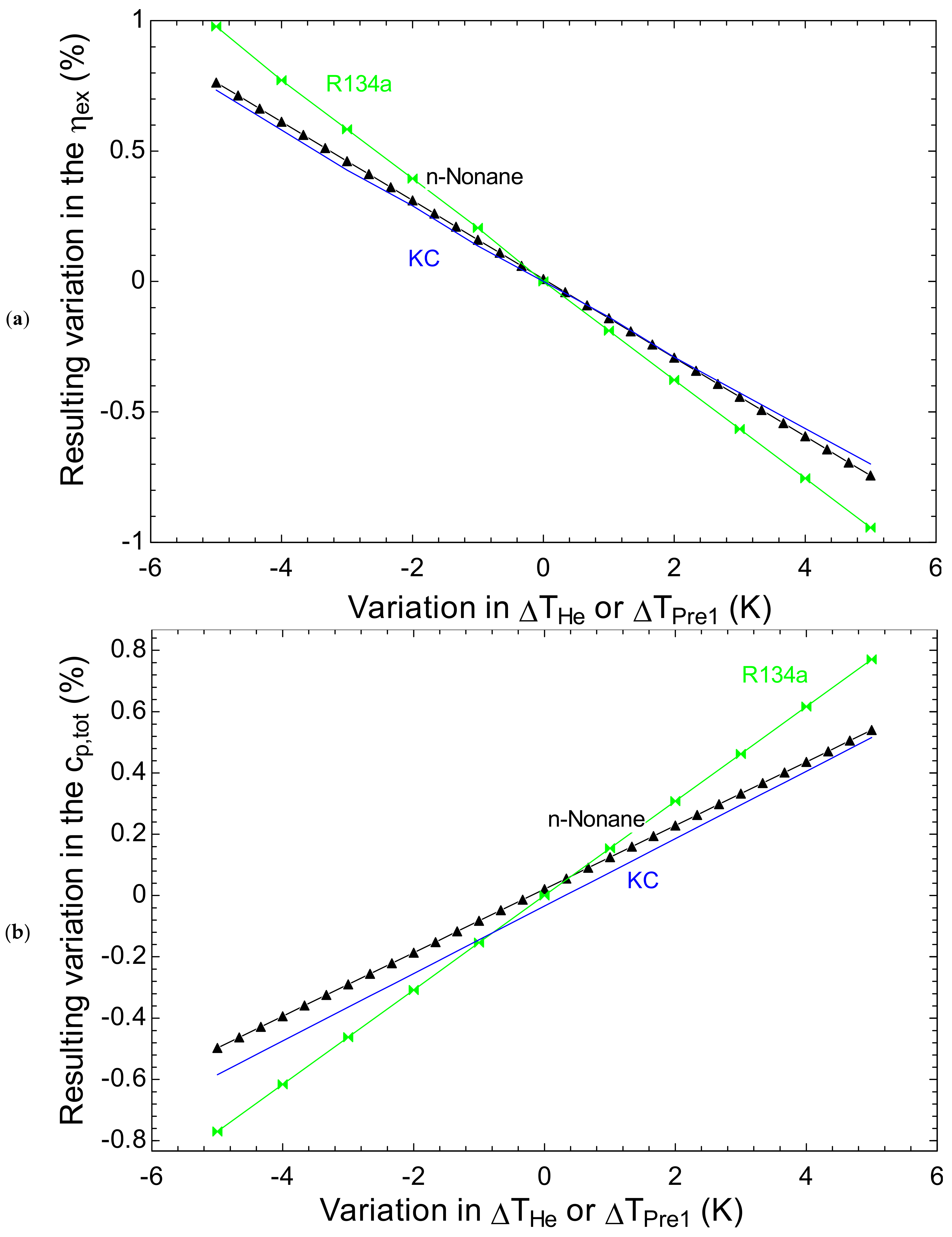
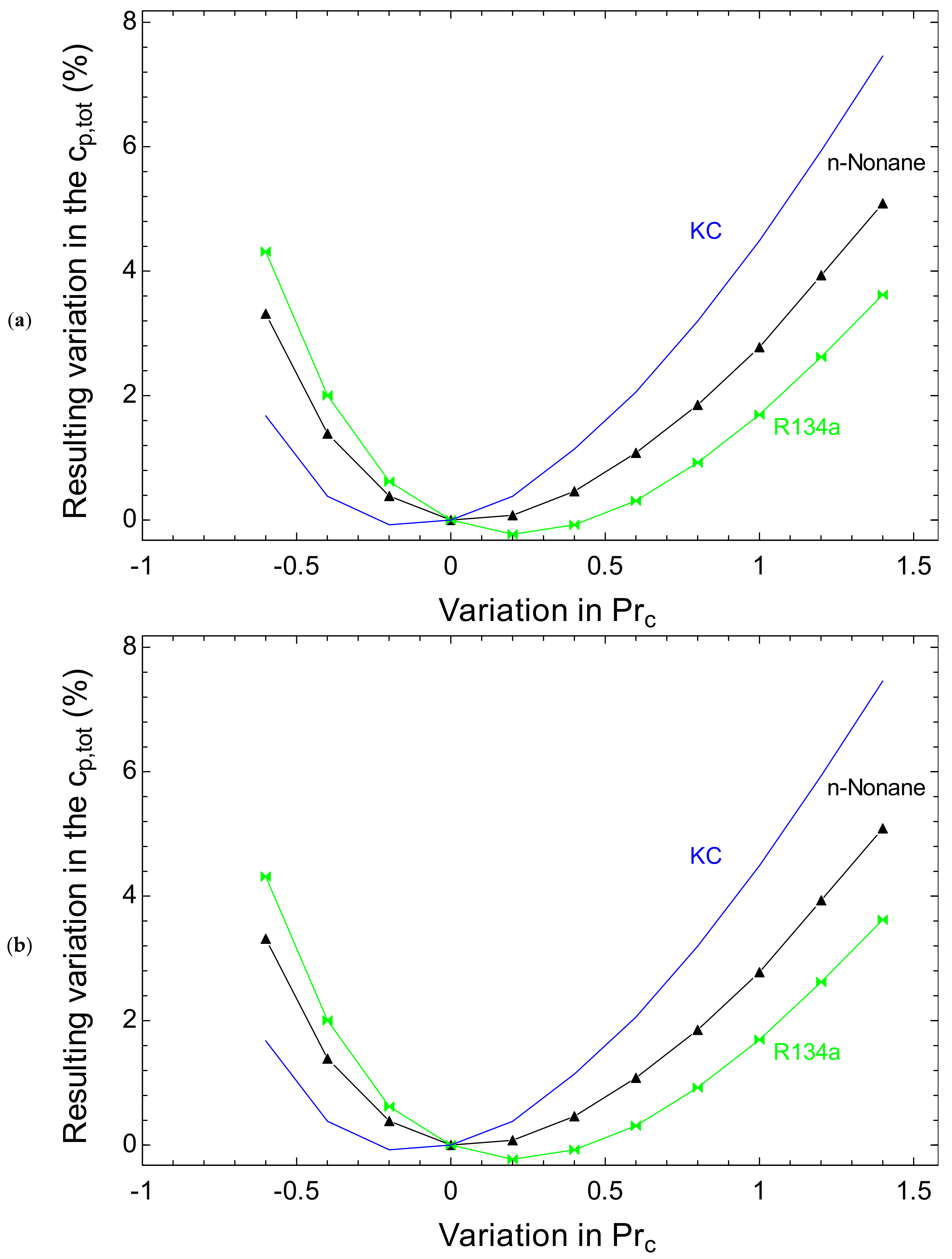
4.5. Sensitivity Analysis

For verifying the sensitivity of the pinch point temperature difference in the heater and pre-cooler 1 and of the compressor pressure ratio on the exergy efficiency and total product unit cost, a sensitivity analysis is performed for the SCRB/OFC, SCRB/ORC and SCRB/KC systems. The results are depicted in Figure 10 and Figure 11, respectively. These figures permit performance sensitivity comparisons of SCRB/ORC, SCRB/OFC and SCRB/KC. For performing the sensitivity analyses, the pinch point temperature difference in the heater and pre-cooler 1 is allowed to range from −5 to 5 K of the initial value for the pinch point temperature difference in the heater and pre-cooler 1 (10 K). The compressor pressure ratio variation considered is from −0.6 to 1.4 relative to its initial value (Pr_c = 2.8). This means, for example, that the compressor pressure ratio is 2.2 when the variation of compressor pressure ratio is −0.6. According to Figure 10, raising the pinch point temperature difference in the heater and pre-cooler 1 has a negative effect on the exergy efficiency and a positive effect on total product unit cost. Referring to Figure 11, by increasing variation of compressor pressure ratio, the exergy efficiency increases at first and then decreases. The exergy efficiency and total product unit cost trends behave opposite to one other. Therefore, increasing the compressor pressure ratio causes the total product unit cost to decrease at first and then to increase. Referring to Figure 10, the resulting variation in the exergy efficiency of the SCRB/ORC system is 1% when variation in pinch point temperature difference is −5 K, which is highest variation. Note that the resulting variations in the exergy efficiencies of SCRB/OFC and SCRB/KC are same and they exhibit almost the same behavior. It is observed in Figure 10b that the highest variation in the total product unit cost is achieved for R134a and is 0.8% when the pinch point temperature difference is 5 K. Again, the behaviors of SCRB/OFC and SCRB/KC are nearly the same. Referring to Figure 11, the lowest resulting exergy efficiency achieved for SCRB/ORC is −8% when the variation in the compressor pressure ratio is −0.6%. Comparing Figure 10 and Figure 11 illustrates that the variations in the compressor pressure ratio affect the resulting variation in the exergy efficiency and total product unit cost much more than the variation in the pinch point temperature in heater or pre-cooler 1.

5. Conclusions

Thermodynamic, exergoeconomic and sustainability analyses are performed successfully for three combined SCRB/OFC, SCRB/ORC and SCRB/KC systems. Ten working fluids are considered for the OFC and ORC systems and, by using a working fluid strategy, the best working fluid from the viewpoints of thermodynamic and economic performances is selected for each system. Parametric studies are carried out for all three systems to determine the effects of decision variables including compressor pressure ratio, bottoming cycle pressure ratio, turbine inlet temperature and pinch point temperature difference in heater or pre-cooler 1 on the second law efficiency and the unit cost of power production. Finally, the performances of the SCRB/OFC, SCRB/ORC and SCRB/KC cycles are optimized and compared. The main results and the conclusions drawn from them are as follows:

(1)

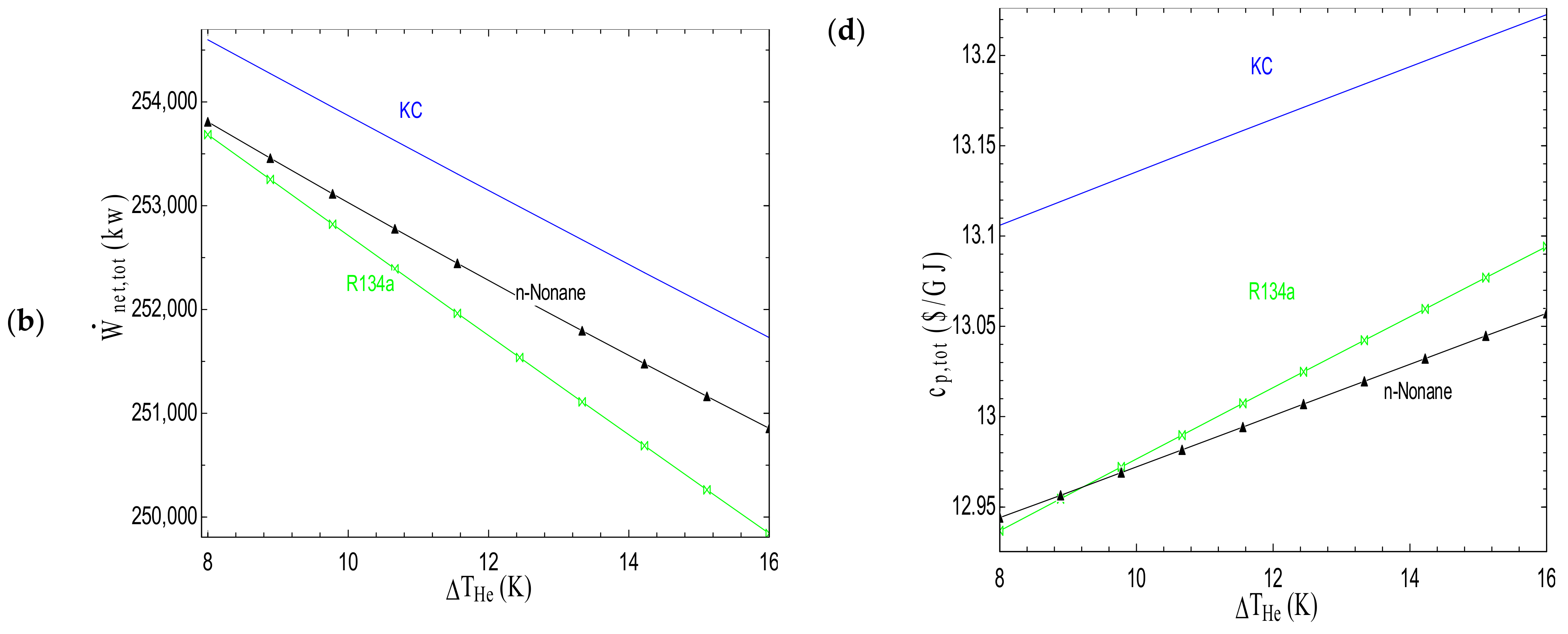
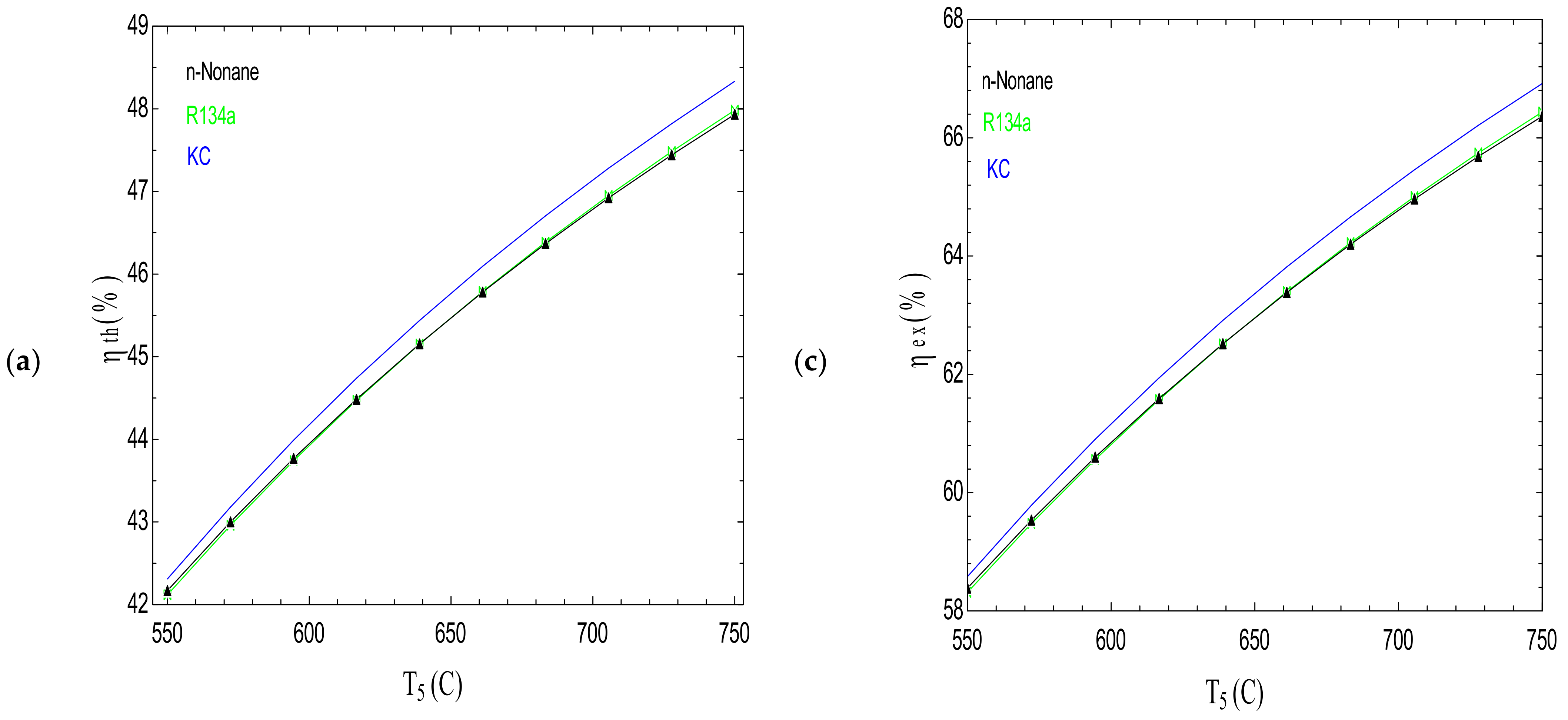
The parametric studies show that the SCRB/OFC, SCRB/ORC and SCRB/KC systems perform thermodynamically and economically better when the pinch point temperature difference is at its own lowest value, which is 8 °C for this work. For achieving more desirable performances for the systems from the viewpoints of thermodynamics and economics, the turbine inlet temperature should be 750 °C, noting that this value is limited by material technology.

(2)

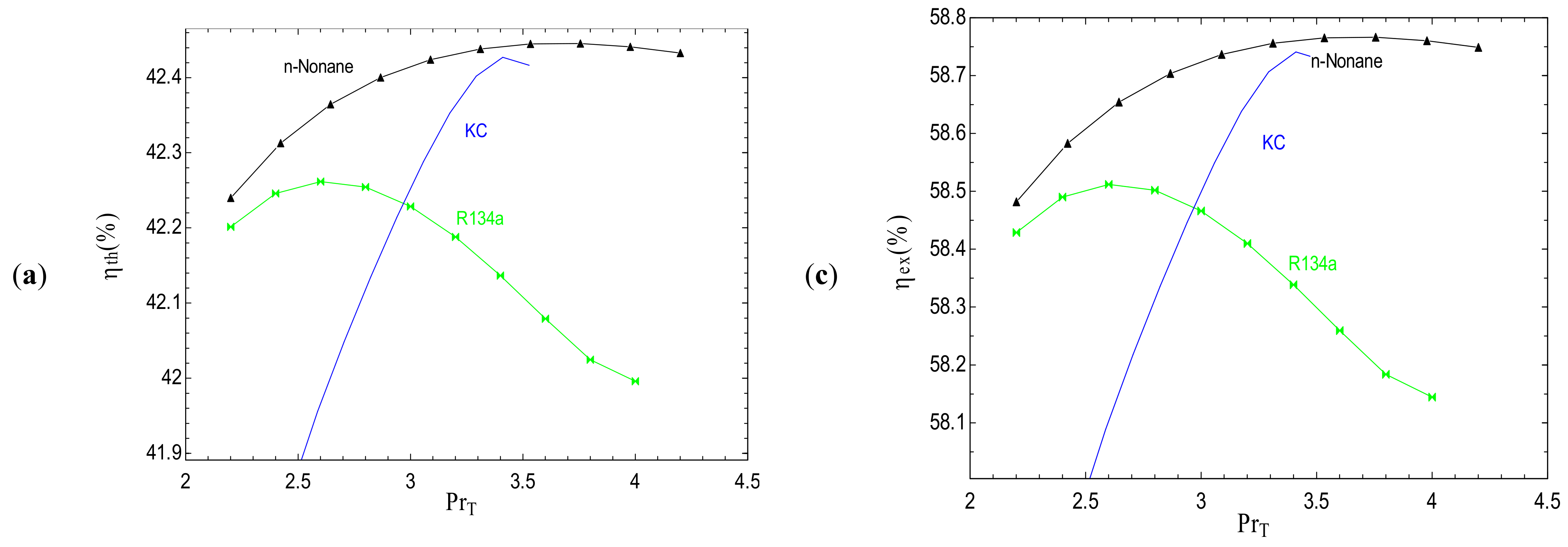
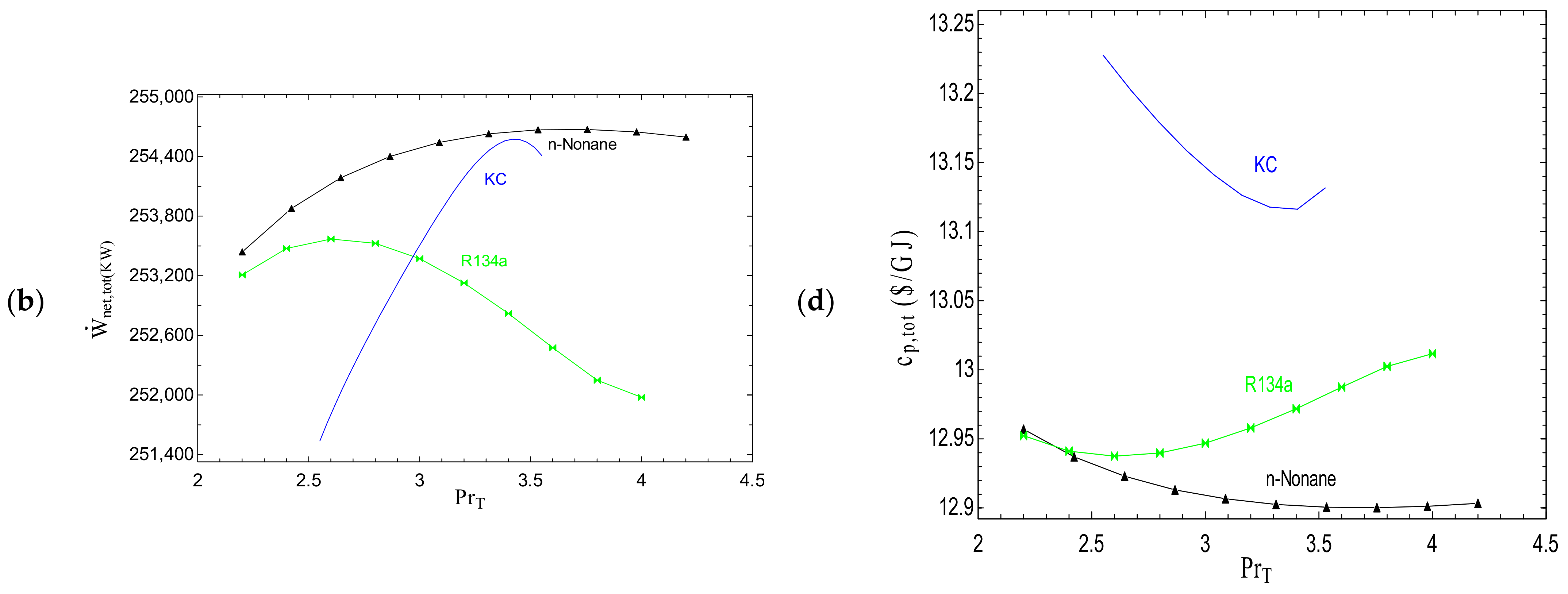
Under the thermodynamic condition of T₅ = 550 °C and ${{\displaystyle \Delta T}}_{He}$ or ${{\displaystyle \Delta T}}_{\mathrm{Pr}e1}$ = 8K, there is an optimum value for the compressor pressure ratio at which the exergy efficiency is maximized and C_{p, total} is minimized.

(3)

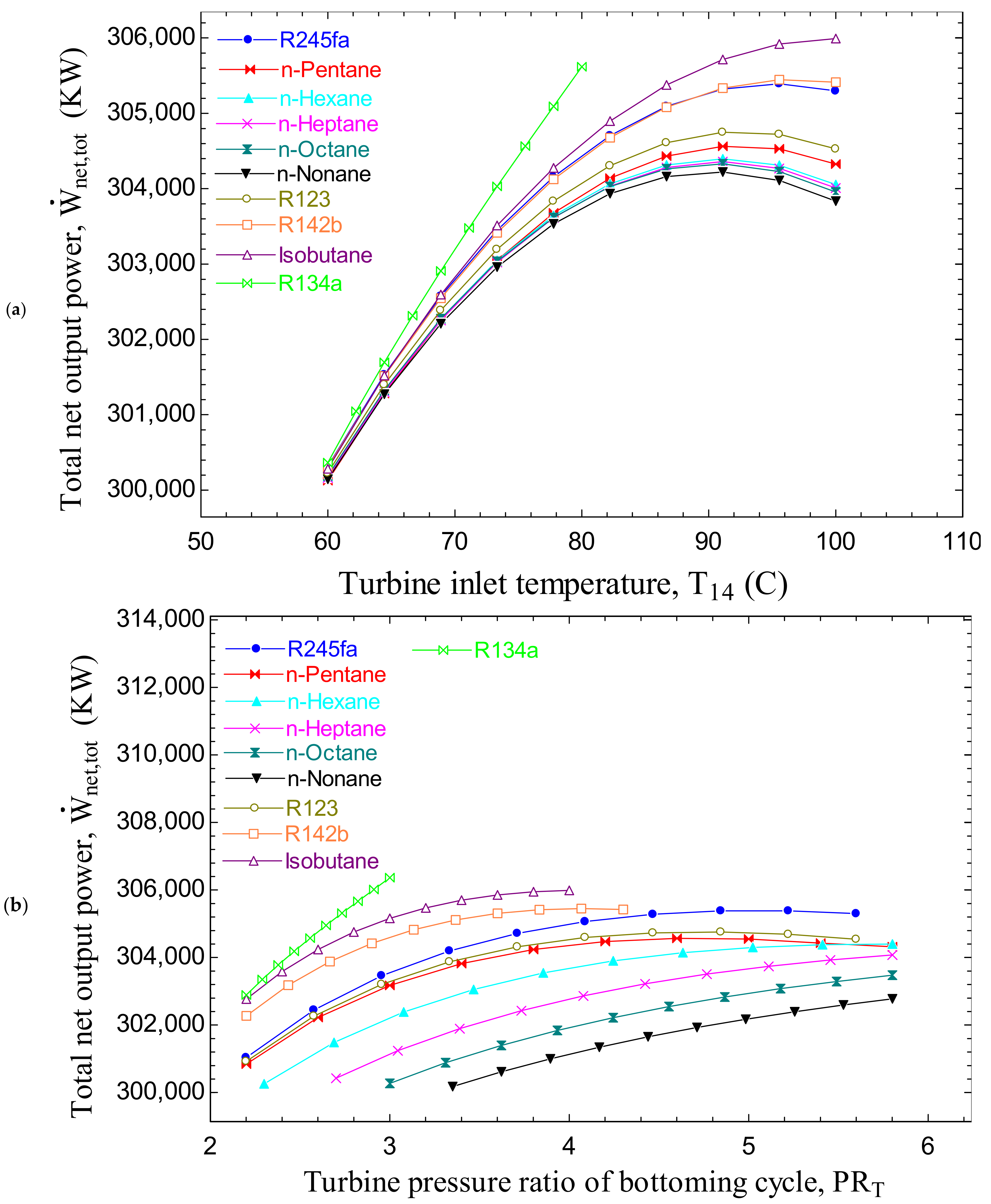
Based on the working fluid selection strategy, the SCRB/OFC and SCRB/ORC cycles achieve their best performances from the viewpoints of exergy and economics, when n-nonane and R134a are used as the working fluid, respectively.

(4)

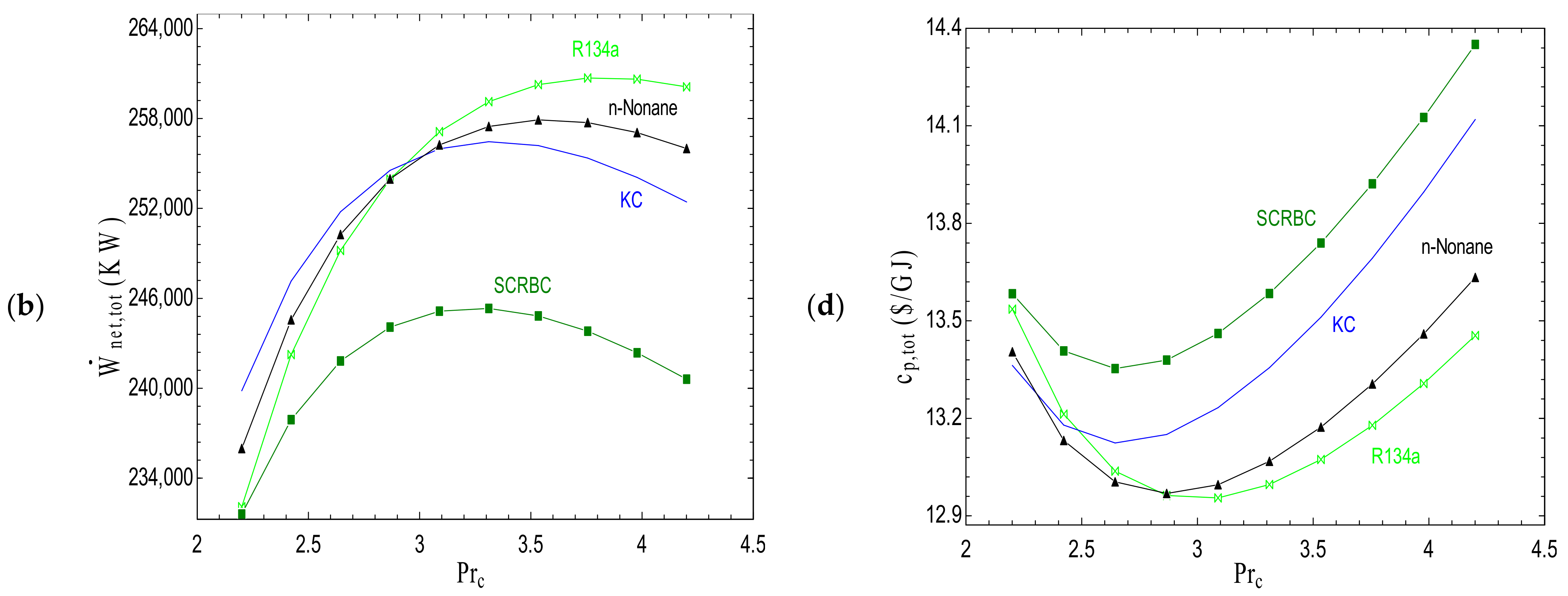
For operation at low pressure ratios, the SCRB/KC cycle exhibits better performance from the viewpoints of thermodynamic and exergoeconomic analyses; however, at high pressure ratios, the SCRB/ORC is the best system.

(5)

The optimization results show that the exergy efficiency of the SCRB/ORC cycle is higher than that of the SCRB/OFC and SCRB/KC cycles, by up to 1.3%. In addition, the unit cost of power production of the SCRB/ORC cycle is lower than those of the SCRB/KC and SCRB/OFC systems by up to 1.9% and 0.75%, respectively.

(6)

The optimization results indicate that the sustainability index for the SCRB/ORC system is 2.48% and 4.62% higher than those for the SCRB/OFC and SCRBB/KC systems, respectively.

(7)

From thermodynamic, exergoeconomic and sustainability perspectives, the SCRB/ORC system is the best option while the SCRB/OFC system can be a promising integrated cycle.

References

1. Sarkar, J. Second law analysis of supercritical CO2 recompression Brayton cycle. Energy 2009, 34, 1172–1178. [Google Scholar] [CrossRef]
2. Zhang, X.R.; Yamaguchi, H.; Uneno, D. Thermodynamic analysis of the CO2-based Rankine cycle powered by solar energy. Int. J. Energy Res. 2007, 31, 1414–1424. [Google Scholar] [CrossRef]
3. Ahn, Y.; Bae, S.J.; Kim, M.; Cho, S.K.; Baik, S.; Lee, J.I.; Cha, J.E. Review of supercritical CO2 power cycle technology and current status of research and development. Nucl. Eng. Technol. 2015, 47, 647–661. [Google Scholar] [CrossRef] [Green Version]
4. Angelino, G. Carbon Dioxide Condensation Cycles For Power Production. J. Eng. Power 1968, 90, 287–295. [Google Scholar] [CrossRef]
5. Dostal, V.; Driscoll, M.J.; Hejzlar, P. A Supercritical Carbon Dioxide Cycle for Next Generation Nuclear Reactors. Master’s Thesis, Massachusetts Institute of Technology, Department of Nuclear Engineering, Cambridge, MA, USA, 2004. [Google Scholar]
6. Dostal, V.; Hejzlar, P.; Driscoll, M.J. The Supercritical Carbon Dioxide Power Cycle: Comparison to Other Advanced Power Cycles. Nucl. Technol. 2006, 154, 283–301. [Google Scholar] [CrossRef]
7. Yari, M.; Mahmoudi, S.M.S. A thermodynamic study of waste heat recovery from GT-MHR using organic Rankine cycles. Heat Mass Transf. 2010, 47, 181–196. [Google Scholar] [CrossRef]
8. Bao, J.; Zhao, L. A review of working fluid and expander selections for organic Rankine cycle. Renew. Sustain. Energy Rev. 2013, 24, 325–342. [Google Scholar] [CrossRef]
9. Besarati, S.M.; Goswami, D.Y. Analysis of Advanced Supercritical Carbon Dioxide Power Cycles with a Bottoming Cycle for Concentrating Solar Power Applications. J. Sol. Energy Eng. 2013, 136, 10904. [Google Scholar] [CrossRef]
10. Akbari, A.D.; Mahmoudi, S.M. Thermoeconomic analysis & optimization of the combined supercritical CO2 (carbon dioxide) recompression Brayton/organic Rankine cycle. Energy 2014, 78, 501–512. [Google Scholar] [CrossRef]
11. Wang, X.; Dai, Y. Exergoeconomic analysis of utilizing the transcritical CO2 cycle and the ORC for a recompression supercritical CO2 cycle waste heat recovery: A comparative study. Appl. Energy 2016, 170, 193–207. [Google Scholar] [CrossRef]
12. Song, J.; Wang, Y.; Wang, K.; Wang, J.; Markides, C.N. Combined supercritical CO2 (SCO2) cycle and organic Rankine cycle (ORC) system for hybrid solar and geothermal power generation: Thermoeconomic assessment of various configurations. Renew. Energy 2021, 174, 1020–1035. [Google Scholar] [CrossRef]
13. Song, J.; Li, X.; Wang, K.; Markides, C.N. Parametric optimisation of a combined supercritical CO2 (S-CO2) cycle and organic Rankine cycle (ORC) system for internal combustion engine (ICE) waste-heat recovery. Energy Convers. Manag. 2020, 218, 112999. [Google Scholar] [CrossRef]
14. Gutierrez, J.C.; Ochoa, G.V.; Duarte-Forero, J. A comparative study of the energy, exergetic and thermo-economic performance of a novelty combined Brayton S-CO2-ORC configurations as bottoming cycles. Heliyon 2020, 6, e04459. [Google Scholar] [CrossRef]
15. Habibi, H.; Zoghi, M.; Chitsaz, A.; Javaherdeh, K.; Ayazpour, M.; Bellos, E. Working fluid selection for regenerative supercritical Brayton cycle combined with bottoming ORC driven by molten salt solar power tower using energy–exergy analysis. Sustain. Energy Technol. Assess. 2020, 39, 100699. [Google Scholar] [CrossRef]
16. Wang, X.; Levy, E.K.; Pan, C.; Romero, C.E.; Banerjee, A.; Rubio-Maya, C.; Pan, L. Working fluid selection for organic Rankine cycle power generation using hot produced supercritical CO2 from a geothermal reservoir. Appl. Therm. Eng. 2018, 149, 1287–1304. [Google Scholar] [CrossRef]
17. Liang, Y.; Bian, X.; Qian, W.; Pan, M.; Ban, Z.; Yu, Z. Theoretical analysis of a regenerative supercritical carbon dioxide Brayton cycle/organic Rankine cycle dual loop for waste heat recovery of a diesel/natural gas dual-fuel engine. Energy Convers. Manag. 2019, 197, 111845. [Google Scholar] [CrossRef]
18. Chen, X.; Pan, M.; Li, X. Novel supercritical CO2/organic Rankine cycle systems for solid-waste incineration energy harvesting: Thermo-environmental analysis. Int. J. Green Energy 2021, 19, 786–807. [Google Scholar] [CrossRef]
19. Wang, Q.; Liu, C.; Luo, R.; Li, D.; Macián-Juan, R. Thermodynamic analysis and optimization of the combined supercritical carbon dioxide Brayton cycle and organic Rankine cycle-based nuclear hydrogen production system. Int. J. Energy Res. 2021, 46, 832–859. [Google Scholar] [CrossRef]
20. Ma, H.; Liu, Z. An Engine Exhaust Utilization System by Combining CO2 Brayton Cycle and Transcritical Organic Rankine Cycle. Sustainability 2022, 14, 1276. [Google Scholar] [CrossRef]
21. Javanshir, A.; Sarunac, N.; Razzaghpanah, Z. Thermodynamic Analysis of ORC and Its Application for Waste Heat Recovery. Sustainability 2017, 9, 1974. [Google Scholar] [CrossRef] [Green Version]
22. Wu, C.; Wang, S.-S.; Li, J. Exergoeconomic analysis and optimization of a combined supercritical carbon dioxide recompression Brayton/organic flash cycle for nuclear power plants. Energy Convers. Manag. 2018, 171, 936–952. [Google Scholar] [CrossRef]
23. Ganesh, N.S.; Srinivas, T. Thermodynamic Assessment of Heat Source Arrangements in Kalina Power Station. J. Energy Eng. 2013, 139, 99–108. [Google Scholar] [CrossRef]
24. Mahmoudi, S.M.S.; Akbari, A.D.; Rosen, M.A. Thermoeconomic Analysis and Optimization of a New Combined Supercritical Carbon Dioxide Recompression Brayton/Kalina Cycle. Sustainability 2016, 8, 1079. [Google Scholar] [CrossRef] [Green Version]
25. Li, H.; Wang, M.; Wang, J.; Dai, Y. Exergoeconomic Analysis and Optimization of a Supercritical CO2 Cycle Coupled with a Kalina Cycle. J. Energy Eng. 2017, 143, 4016055. [Google Scholar] [CrossRef]
26. Feng, Y.; Du, Z.; Shreka, M.; Zhu, Y.; Zhou, S.; Zhang, W. Thermodynamic analysis and performance optimization of the supercritical carbon dioxide Brayton cycle combined with the Kalina cycle for waste heat recovery from a marine low-speed diesel engine. Energy Convers. Manag. 2020, 206, 112483. [Google Scholar] [CrossRef]
27. Sadeghi, M.; Nemati, A.; Ghavimi, A.; Yari, M. Thermodynamic analysis and multi-objective optimization of various ORC (organic Rankine cycle) configurations using zeotropic mixtures. Energy 2016, 109, 791–802. [Google Scholar] [CrossRef]
28. Roy, J.; Mishra, M.; Misra, A. Parametric optimization and performance analysis of a waste heat recovery system using Organic Rankine Cycle. Energy 2010, 35, 5049–5062. [Google Scholar] [CrossRef]
29. Sadeghi, M.; Chitsaz, A.; Marivani, P.; Yari, M.; Mahmoudi, S. Effects of thermophysical and thermochemical recuperation on the performance of combined gas turbine and organic rankine cycle power generation system: Thermoeconomic comparison and multi-objective optimization. Energy 2020, 210, 118551. [Google Scholar] [CrossRef]
30. Lemmon, E.W.; Huber, M.L.; McLinden, M.O. REFPROP Version 8.0: Reference Fluid Thermodynamic and Transport Properties; NIST Standard Reference Database 23; National Institute of Standards and Technology: Gaithersburg, MD, USA, 2007. [Google Scholar]
31. Aljundi, I.H. Effect of dry hydrocarbons and critical point temperature on the efficiencies of organic Rankine cycle. Renew. Energy 2011, 36, 1196–1202. [Google Scholar] [CrossRef]
32. Malafeev, I.I.; Il’In, G.A.; Sapozhnikov, V.B. Mathematical-Experimental Assessment of Energy Efficiency of High-Temperature Heat Pump Distiller. Chem. Pet. Eng. 2019, 55, 556–561. [Google Scholar] [CrossRef]
33. Nemati, A.; Nami, H.; Yari, M. Assessment of different configurations of solar energy driven organic flash cycles (OFCs) via exergy and exergoeconomic methodologies. Renew. Energy 2018, 115, 1231–1248. [Google Scholar] [CrossRef]
34. Wu, C.; Wang, S.-S.; Feng, X.-J.; Li, J. Energy, exergy and exergoeconomic analyses of a combined supercritical CO 2 recompression Brayton/absorption refrigeration cycle. Energy Convers. Manag. 2017, 148, 360–377. [Google Scholar] [CrossRef]
35. Sarkar, J.; Bhattacharyya, S. Optimization of recompression S-CO2 power cycle with reheating. Energy Convers. Manag. 2009, 50, 1939–1945. [Google Scholar] [CrossRef]
36. Lee, H.Y.; Park, S.H.; Kim, K.H. Comparative analysis of thermodynamic performance and optimization of organic flash cycle (OFC) and organic Rankine cycle (ORC). Appl. Therm. Eng. 2016, 100, 680–690. [Google Scholar] [CrossRef]
37. Dincer, I.; Rosen, M.A. Exergy: Energy, Environment and Sustainable Development, 3rd ed.; Elsevier: Oxford, UK, 2021. [Google Scholar]
38. Schultz, K.; Brown, L.; Besenbruch, G.; Hamilton, C. Large-Scale Production of Hydrogen by Nuclear Energy for the Hydrogen Economy; General Atomics: San Diego, CA, USA, 2003. [Google Scholar] [CrossRef] [Green Version]
39. Bejan, A.; Tsatsaronis, G.; Moran, M.J. Thermal Design and Optimization; John Wiley & Sons: New York, NY, USA, 1995. [Google Scholar]
40. Lazzaretto, A.; Tsatsaronis, G. SPECO: A systematic and general methodology for calculating efficiencies and costs in thermal systems. Energy 2006, 31, 1257–1289. [Google Scholar] [CrossRef]
41. Sarabchi, N.; Yari, M.; Mahmoudi, S.S. Exergy and exergoeconomic analyses of novel high-temperature proton exchange membrane fuel cell based combined cogeneration cycles, including methanol steam reformer integrated with catalytic combustor or parabolic trough solar collector. J. Power Source 2020, 485, 229277. [Google Scholar] [CrossRef]
42. Byun, M.; Kim, H.; Choe, C.; Lim, H. Conceptual feasibility studies for cost-efficient and bi-functional methylcyclohexane dehydrogenation in a membrane reactor for H2 storage and production. Energy Convers. Manag. 2020, 227, 113576. [Google Scholar] [CrossRef]
43. Dincer, I.; Joshi, A.S. Solar Based Hydrogen Production Systems; Springer: Cham, Switzerland, 2013. [Google Scholar] [CrossRef]
44. Ahmadi, P.; Dincer, I.; Rosen, M.A. Exergo-environmental analysis of an integrated organic Rankine cycle for trigeneration. Energy Convers. Manag. 2012, 64, 447–453. [Google Scholar] [CrossRef]
45. Nami, H.; Ranjbar, F.; Yari, M. Thermodynamic assessment of zero-emission power, hydrogen and methanol production using captured CO2 from S-Graz oxy-fuel cycle and renewable hydrogen. Energy Convers. Manag. 2018, 161, 53–65. [Google Scholar] [CrossRef]
46. LaBar, M.P. The gas turbine–modular helium reactor: A promising option for near term deployment. In Proceedings of the International Congress on Advances in Nuclear Power Plants, Hollywood, FL, USA, 9–13 June 2002. [Google Scholar]
47. Zare, V.; Mahmoudi, S.; Yari, M. On the exergoeconomic assessment of employing Kalina cycle for GT-MHR waste heat utilization. Energy Convers. Manag. 2015, 90, 364–374. [Google Scholar] [CrossRef]
48. Mosaffa, A.; Zareei, A. Proposal and thermoeconomic analysis of geothermal flash binary power plants utilizing different types of organic flash cycle. Geothermics 2018, 72, 47–63. [Google Scholar] [CrossRef]
49. Vieira, L.S.; Donatelli, J.L.; Cruz, M.E. Exergoeconomic improvement of a complex cogeneration system integrated with a professional process simulator. Energy Convers. Manag. 2009, 50, 1955–1967. [Google Scholar] [CrossRef]
50. Guo-Yan, Z.; En, W.; Shan-Tung, T. Techno-economic study on compact heat exchangers. Int. J. Energy Res. 2008, 32, 1119–1127. [Google Scholar] [CrossRef]
51. Dorj, P. Thermoeconomic Analysis of a New Geothermal Utilization CHP Plant in Tsetserleg, Mongolia. Master’s Thesis, University of Iceland, Departement of Mechanical and Industrial Engineering, Reykjavík, Iceland, 2005. [Google Scholar]
Figure 1. Schematic of proposed SCRB/OFC system.
Sustainability 14 08769 g001
Figure 2. Schematic of proposed SCRB/ORC system.
Sustainability 14 08769 g002
Figure 3. Schematic of proposed SCRB/KC system.
Sustainability 14 08769 g003
Figure 4. Effects of OFC turbine inlet temperature (a) and OFC turbine pressure ratio (b) in bottoming cycle of SCRB/OFC for high temperature waste heat recovery condition on the total net output power of SCRB/OFC.
Sustainability 14 08769 g004
Figure 5. Effects of ORC turbine inlet temperature (a) and ORC turbine pressure ratio (b) in bottoming cycle of SCRB/ORC for high temperature waste heat recovery condition on the total net output power of SCRB/ORC.
Sustainability 14 08769 g005
Figure 6. Effects of compressor pressure ratio on first law efficiency (a), total net output power (b), second law efficiency (c) and total product unit cost (d) for three integrated cycles (T5 = 550 °C and Δ T H e or Δ T Pr e 1 = 10 K).
Sustainability 14 08769 g006aSustainability 14 08769 g006b
Figure 7. Effects of the pinch point temperature difference in heater and pre-cooler 1 on first law efficiency (a), total net output power (b), second law efficiency (c) and total product unit cost (d) for three integrated cycles. (T5 = 550 °C and Prc = 2.8).
Sustainability 14 08769 g007aSustainability 14 08769 g007b
Figure 8. Effects of turbine inlet temperature on first law efficiency (a), total net output power (b), second law efficiency (c) and total product unit cost (d) for three integrated cycles (Prc = 2.8 and Δ T H e or Δ T Pr e 1 = 10 K).
Sustainability 14 08769 g008aSustainability 14 08769 g008b
Figure 9. Effects of turbine pressure ratio of bottoming cycle on first law efficiency (a), total net output power (b), second law efficiency (c) and total product unit cost (d) for three integrated cycles (Prc = 2.8, T5 = 550 °C and Δ T H e or Δ T Pr e 1 = 10 K).
Sustainability 14 08769 g009aSustainability 14 08769 g009b
Figure 10. Sensitivity analysis results, showing effect of pinch point temperature difference in heater and pre-cooler 1 on exergy efficiency (a) and total product unit cost (b).
Sustainability 14 08769 g010
Figure 11. Sensitivity analysis results, showing effect of compressor ratio on exergy efficiency (a) and total product unit cost (b).
Sustainability 14 08769 g011