Predicting Pavement Structural Condition Using Machine Learning Methods

Abstract

State departments of transportation recognize the need to incorporate pavement structural condition in their pavement performance models and/or decision processes used to select candidate projects for preservation, rehabilitation, or reconstruction at the network level. However, pavement structural condition data are costly to obtain. To this end, this paper develops and evaluates the effectiveness of two machine learning methods, Random Forest (RF) and eXtreme Gradient Boosting (XGBoost), for predicting a flexible pavement’s structural condition. The aim is to be able to predict whether a pavement section’s structural condition is poor or not based on Annual Average Daily Traffic (AADT), truck percentage, and speed limit. The structural condition of a pavement is considered poor if the Surface Curvature Index (SCI₁₂) is above 3.3. The models are developed using 950 miles of Traffic Speed Deflectometer (TSD) data collected along 8 primary routes in South Carolina. The performance of the machine learning models was compared with that of a logistic regression model. When the trained models are applied to the test data, the prediction results indicated that the XGBoost and RF models outperform the logistic regression model by 12% and 8%, respectively. XGBoost outperformed RF by 4%. With XGBoost found to be the best among the three models evaluated, its performance was examined using other poor structural condition threshold values; its prediction accuracy is found to be robust across the different scenarios. AADT and truck percentages are found to be significant factors whereas speed limit has no effect on a pavement’s structural condition.

1. Introduction

Currently, most state departments of transportation (DOTs) rely only on the pavement functional condition data to select candidate projects for preservation, rehabilitation, or reconstruction at the network level [1]. A pavement’s functional condition is related to roughness and surface distresses, whereas a pavement’s structural condition is related to its strength or carrying capacity. As part of this study, a survey of state DOTs was conducted which had 25 responses. The responses indicated that only 13% of the respondents currently use structural condition data to make decisions at the network level, and 47.8% of the respondents plan to use structural condition data in the future. Previous studies have found that there is little correlation between a pavement’s functional condition and a pavement structural condition [2,3]. Using South Carolina DOT’s Traffic Speed Deflectometer (TSD) data, this study arrived at the same conclusion. Specifically, it was found that 50% has low Pearson correlation (below ±0.29), 27.5% has moderate correlation (between ±0.30 and ±0.49), and 22.5% has high correlation (between ±0.5 and ±1.0). This finding confirmed prior knowledge that a pavement’s functional condition does not accurately portray its underlying condition related to remaining service life or the potential for future deterioration. For this reason, a number of researchers have recommended the consideration of both pavement functional and structural condition for pavement management [4,5,6,7].

To obtain pavement structural condition data, one approach involves the use of Falling Weight Deflectometer (FWD). The major limitations of this device are: (1) FWD operates at slow speed and measures pavement deflection at discrete points along the pavement sections and thus does not provide the complete profile of the roadway, and (2) this device requires lane closures that disrupt traffic operations. These limitations make FWD unsuitable to be used at the network level for pavement management [1,8]. In contrast, TSD measures pavement deflections continuously at traffic speed rather than at discrete points and does not require lane closures like FWD [9,10]. Several state DOTs have begun to explore the use of TSD data, including South Carolina DOT (SCDOT) from which this study is based.

The use of TSD in the U.S. is fairly new; thus, research involving the use of TSD data is limited. These studies can be grouped into three categories: (1) how to classify pavement structural condition using TSD data, (2) how to use TSD data for pavement management, and (3) how to use TSD data to predict pavement structural condition. For category 1, several studies have proposed indicators and threshold values to quantify a pavement’s structural condition as good, fair, or poor. Shrestha et al. [1] proposed the use of Surface Curvature Index (SCI₃₀₀) to predict a pavement’s structural condition and developed threshold values for this indicator. This particular indicator (SCI₃₀₀) is directly related to TSD data, whereas other studies proposed indicators that are based on FWD data. Manoharan et al. [9] proposed the use of Adjusted Structural Number, Shrestha et al. [11] proposed the use of Deflection Slope Index (DSI), and Manoharan et al. proposed the use of Remaining Structural Life [12]. For category 2, only the work by Shrestha et al. [1] has investigated the use of pavement structural condition data for system-wide pavement management. For category 3, Shrestha et al. [11] developed a pavement deterioration model based on pavement age and DSI, and Zihan et al. [13] developed a non-linear model to predict a pavement’s Structural Number (SN). To date, no study has investigated the use of machine learning models to predict a pavement’s structural condition. Since machine learning models are not constrained by a specific model structure and can handle large data sets with any degree of complexity [14], they may be more suitable than traditional parametric methods.

The objective of this paper is to develop two machine learning models, eXtreme Gradient Boosting (XGBoost) and Random Forest (RF), to predict a pavement’s structural condition using influencing factors with readily available data: Annual Average Daily Traffic (AADT), truck percentage, and speed limit. Such a model will assist state highway agencies, counties, and municipalities in incorporating structural condition into pavement performance models or decision processes used to select candidate projects at the network level. The models’ performances are compared with each other and that of a traditional parametric approach, logistic regression, using TSD data from South Carolina.

The remainder of this paper is organized as follows. Section 2 provides a summary of recent transportation studies that applied machine learning models to illustrate their diverse applications. Section 3 discusses the source of the TSD data, and the procedure taken to prepare the data for modeling. Section 4 presents the mathematical details of RF and XGBoost, as well as that of the logistic regression. Section 5 presents and discusses the prediction results of the three models. Lastly, Section 6 provides a summary of the study and concluding remarks.

2. Literature Review

Machine learning, a form of Artificial Intelligence (AI), has been applied widely in transportation applications. Its popularity is due to its ability to learn the latent patterns of historical data to model the behavior of a system. With more data being collected by various sensors, providing much larger data sets than ever before, and recent advances to computing technologies, machine learning-based approaches are emerging as viable tools to solve complex problems in transportation. The following highlights some example applications of machine learning approaches in transportation and pavement condition.

Kim et al. [15] applied aggregated channel feature (ACF) and faster region-based convolutional neural network (Faster R-CNN) to obtain accurate vehicle trajectories in congested traffic using a camera mounted on Unmanned aerial vehicles (UAVs). Luo et al. [16] combined the k-nearest neighbor (KNN) approach with the long short-term memory network (LSTM) approach to predict traffic flow to improve the effectiveness of Intelligent Transportation Systems. Eraqi et al. [17] proposed the use of a learnable weighted ensemble of convolutional neural networks (CNNs) to detect distracted driving in real-time. Xue et al. [18] evaluated the effectiveness of Support Vector Machine (SVM) to detect driving style that contributed to rear-end collisions to improve the design of driver assistance systems and vehicle control systems. Shang et al. [19] proposed to combine Neighborhood Components Analysis (NCA) and the Bayesian Optimization Algorithm (BOA)-optimized Random Forest (RF) model to predict traffic incident duration. Sun et al. [20] applied the gradient boosting decision tree algorithm to predict driving range of battery electric vehicles. Lastly, Cheng et al. [21] applied Random Forests (RF) to predict travel time to improve route guidance systems.

Many studies have shown that artificial neural networks outperformed multiple linear regression in predicting International Roughness index (IRI). A recent study of such work and related references can be found in the work by Abdelaziz et al. [22]. Kaloop et al. [23] integrated Optimally Pruned Extreme Learning Machine (OP-ELM) and Wavelet analysis to improve the OP-ELM results and designed a novel hybrid Wavelet-OPELM (WOPELM) model for predicting International Roughness Index (IRI). Guo et al. [24] proposed an ensemble learning model that utilized a Gradient Boosting Decision Tree (GBDT) to predict IRI and rut depth. To date, only the work by Karballaeezadeh et al. [25] has attempted to predict pavement structural numbers. They evaluated the performance of Gaussian process regression, M5P model tree, and random forest to predict structural numbers of flexible pavements based on surface deflections and surface temperature. Readers are referred to the review paper by Justo-Silva et al. [26] for other machine learning techniques that have been applied to pavement condition modeling.

The above review illustrates the variety of machine learning approaches that have been applied in transportation and pavement performance prediction, all of which were shown to be effective for their particular application and context. The two approaches selected for this study are gradient boosting and random forest. They are motivated by the work of Guo et al. [24], who demonstrated the potential of Gradient Boosting Decision Tree for predicting IRI, and Karballaeezadeh et al. [25], who showed that the random-forest algorithm produced comparable results to more sophisticated methods in predicting pavement structural numbers. As noted previously, this study is the first to evaluate the performance of these models to predict a pavement’s structural condition using TSD data.

3. Data Description

3.1. Source of TSD Data

TSD is a continuous pavement deflection-measuring device that measures pavement response to an applied load. It was developed by Greenwood Engineering in the early 2000′s using doppler laser-based technology. TSDs are being used by many transportation agencies around the world. As part of the pooled fund studies (i.e., TPF-5(282) and 5(385)), the SCDOT obtained TSD data for approximately 950 miles along 8 primary routes in the state of South Carolina. A map of the routes selected by SCDOT to obtain TSD data for is shown in Figure 1. The length of TSD measurements obtained for each route is summarized below, in descending order.

• SC-9: 231 miles
• US-321: 216 miles
• US-378: 201 miles
• US-178: 181 miles
• US-29: 37 miles
• US-78: 36 miles
• US-17: 19 miles
• US-501: 12 miles

The TSD data were obtained by the Australian Road Research Board (ARRB) with its Intelligent Pavement Assessment Vehicle (IPAVe). IPAVe (shown in Figure 2) is a semi-trailer truck that is equipped with six Doppler sensors to measure pavement deflection located at 110 mm (~4 in.), 210 mm (~8 in.), 310 mm (~12 in.), 610 mm (~24 in.), 910 mm (~36 in.), and 1510 mm (~60 in.) from the center of the wheel load. The pavement structural condition index or surface curvature index (SCI) can be derived from the deflection slope. In this study, SCI₁₂ is used to quantify pavement structural condition. It is the difference between D₀ and D₁₂, where D₀ is the maximum deflection (under the applied load) and D₁₂ is the deflection at 12 in (or 300 mm) from the applied load.

3.2. Data Preparation

The TSD data were collected in 2019 at 0.01-mile increments by IPAVe, which used the World Geodetic System (WGS84) coordinate system. The SCDOT’s roadway and traffic data, such as annual average daily traffic (AADT), are available in the North American Datum (NAD83) coordinate system. To enable the modeling of TSD data with respect to SCDOT roadway and traffic data, ESRI’s ArcMap 10.8.1 was used to convert TSD data from WGS84 to NAD83, and a Python program was developed to pair TSD data with roadway data by segments. The SCDOT defines segments as those with common pavement quality, AADT, and number of lanes.

SCI₁₂ was used to quantify a pavement as good, fair, or poor. To accomplish this, the SCDOT’s documented percentages of good, fair, and poor pavement for non-interstate National Highway System based on federal guidelines were used as a reference. It should be noted that these percentages were used because they correspond to the State Pavement Engineer’s assessment of the state’s pavement condition through FWD testing and core samples. From these percentages, the SCI₁₂ values were back-calculated to provide the same percentages of good, fair, and poor. The SCI₁₂ threshold values shown in

Table 1. SCI₁₂ thresholds for classifying pavement structural condition.

Pavement Condition	Percentage	SCI12 Thresholds
Good	28%	<1.6
Fair	27%	1.6–3.3
Poor	45%	>3.3

demarcate the distribution of SCI₁₂ data such that 28% of TSD route segments have SCI values less than 1.6 and are considered good; 27% have SCI₁₂ values between 1.6 and 3.3 and are considered fair; and 45% have SCI₁₂ values above 3.3, which are considered poor.

Based on the specified thresholds, there are 18.38% segments with good pavement, 30.12% with fair pavement, and 51.5% with poor pavement. Due to the need to have a balanced dataset when applying machine learning models, two categories are used instead of three. Specifically, the good and fair categories are combined, resulting in poor and non-poor pavement categories that we wish to predict with readily available roadway and traffic data.

Previous studies conducted by Rahman et al. [27] and Kim and Kim [28] indicated that AADT has an effect on pavement deterioration, Lu et al. [29], Chou et al. [30], and Salama et al. [31] indicated that the percentage of trucks has an effect on pavement deterioration, and Mshali and Steyn [32] indicated that the speed limit has an effect of pavement deterioration. Thus, these factors are considered as explanatory variables in the models evaluated in this study.

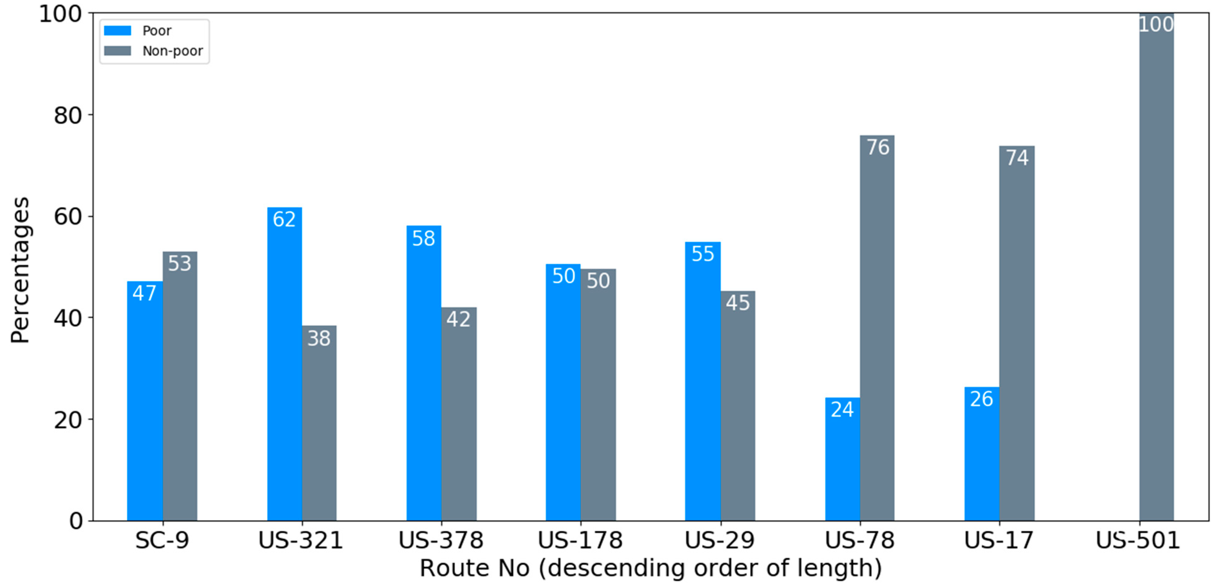
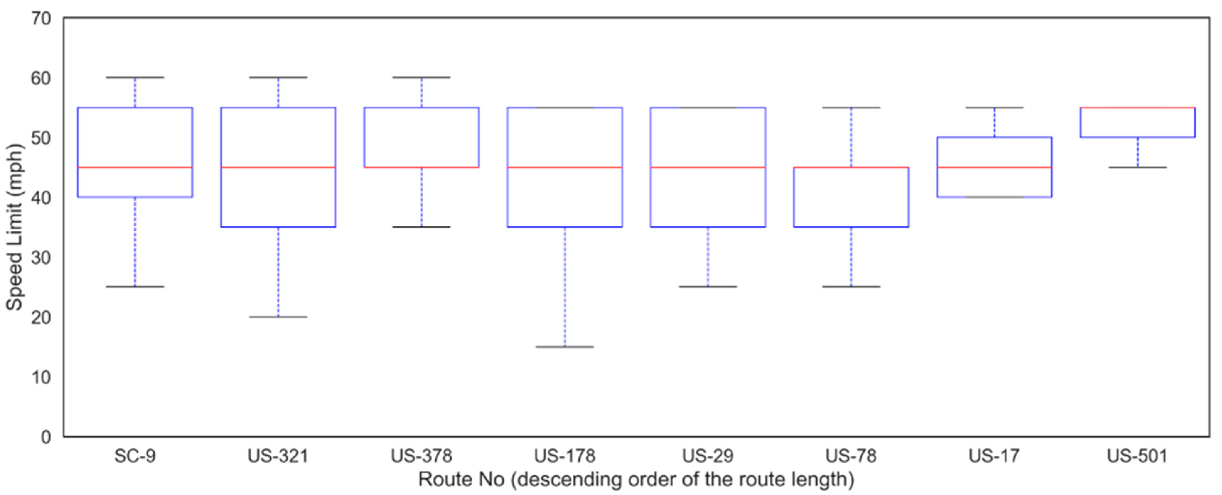
3.3. Descriptive Statistics

Figure 3 shows the percentages of poor and non-poor pavement segments for each route. Collectively, there are 8 routes with TSD data and 800 pavement segments. Overall, 51.5% of pavement segments have poor structural condition, and 48.5% have non-poor structural condition. Note that these percentages yield a balanced dataset necessary for training machine learning models. The three routes with shortest length are US-78, US-17, and US-501, and their lengths are 36, 19, and 12 miles, respectively. These three routes have a greater percentage of non-poor structural condition relative to the other routes. US-178 has equal percentages of poor and non-poor pavement segments. The three routes with longest length are SC-9, US-321, and US-378, and their lengths range from 200 to 231 miles. Among the three longest routes, SC-9 has a larger percentage of segments with non-poor structural condition.

Figure 4, Figure 5 and Figure 6 show boxplots of AADT, truck percentage, and speed limit for each route, respectively. The red line in the boxplot denotes the median value (50th percentile), the blue box denotes the inter-quantile range from 25th percentile to 75th percentile, and the two whiskers denote the 90% range, from 5th percentile to 95th percentile. It can be seen from the boxplots that the shortest two routes (US-17 and US-501) have significantly higher AADT than the other routes, and the three longest routes have relatively higher truck percentages. As shown, the mean speed limit is either 45 mph (miles per hour) or 55 mph, but there is considerable variation in speed. Take US-178, for example: some segments on it have speed limits as low as 15 mph while others have speed limits of 55 mph. Figure 7 shows the distributions of SCI₁₂ values along 0.1-mile sub-segments for each route. It can be seen that most routes have a widespread distribution of SCI₁₂.

4. Methods

The following provides a brief overview of RF, XGBoost, and logistic regression. Readers are referred to the work of Jiang et al. [33] for a comprehensive explanation of RF, Gong et al. [34] for explanation of XGBoost, and Rezapour et al. [35] for an explanation of logistic regression. With each of these models, the goal is to predict a pavement’s structural condition, specifically whether it is poor or non-poor; thus, the response variable has only two outcomes. The explanatory variables used to predict the outcome are AADT, truck percentage, and speed limit of each segment. Climatic conditions were not included in the models because the TSD data were collected within a period of four days. Other variables such as soil conditions, pavement structure, and age were available for only a subset of the segments. Including these variables would have resulted in a sample too small for machine learning models.

4.1. Random Forest

Random forest (RF) is a tree-based algorithm which involves building several trees (decision trees), then combining their output to improve generalization ability of the model. The method of combining trees is known as an ensemble method. The algorithm works by growing M different (randomized) trees as follows [36]. Prior to the construction of each tree, n observations are drawn at random with (or without) replacement from the original data set. These—and only these—n observations (with possible repetitions) are taken into account in the tree building. Then, at each node of each tree, a split is performed by maximizing the Gini index (i.e., a measure of node purity) or entropy (i.e., a measure of node impurity) over mtry directions chosen uniformly at random among the p original ones; mtry is the number of possible directions for splitting at each node of each tree. Lastly, construction of individual trees is stopped when each node contains less than nodesize points; nodesize is the number of records in each node below which the node is not split. Thus, implementing RF requires determination of the total number of trees to grow, number of randomly selected variables (mtry) at a node split, and maximum tree depth (governed by nodesize).

4.2. eXtreme Gradient Boosting (XGBoost)

eXtreme Gradient Boosting Decision Tree (XGBoost) is an improvement of the Gradient Boosting algorithm proposed by Chen and Guestrin [37]. The theoretical basis of XGBoost is as follows. Suppose the model has k decision trees, the integrated model can be expressed mathematically as [38]:

$${\widehat{y}}_i={\displaystyle \sum _{k=1}^t{f}_k(x_i)}$$

where t is the set of regression trees and f_k is a regression tree in the set. The main idea of XGBoost algorithm is that each update is based on the prediction results of the previous model. By adding a new tree f_k to fit the residual error between the predicted value of the previous tree and the actual value, a new model is formed, and the new model is used as the basis for the next model learning. Mathematically, this can be stated as follows [38].

$${\stackrel{\wedge }{y_i}}^{(t)}={\stackrel{\wedge }{y}}_i{}^{(t-1)}+f_t(x_i)$$

(1)

where ${\stackrel{\wedge }{y_i}}^{(t)}$ is the predicted value at time t, ${\stackrel{\wedge }{y_i}}^{(t-1)}$ is the predicted value at time (t − 1), $f_t(x_i)$ is the residual fitting value by the newly added regression tree, and $x_i$ is input data.

To obtain as close as possible to the true value of y_i, the following objective function is minimized by the XGBoost algorithm [38].

$$ob{j}^{(t)}=l\left(y_i,{\widehat{y}}_i^{(t)}\right)+{\gamma }^T+\frac{1}{2}\lambda {\displaystyle \sum _{j=1}^T{w}_j^2}$$

(2)

The first term in the objective function represents the error function, also known as the loss function. The remaining terms represent the regularization where T represents the number of leaf nodes in the tree and the second part represents the L2 modulus square of the weight function w of the leaf nodes in the tree.

4.3. Logistic Regression

A logistic regression is a special case of multiple regression where the response variable (also known as dependent variable) has only two outcomes. Mathematically, it is expressed as [35]:

$$\ln (\frac{P_n(i)}{1-P_n(i)})={\beta }_0+{\beta }_1{x}_1+{\beta }_2{x}_2+{\beta }_3{x}_3+\dots \dots \dots \dots +{\beta }_p{x}_p$$

(3)

$$\frac{P_n(i)}{1-P_n(i)}=\exp ({\beta }_0+{\beta }_1{x}_1+{\beta }_2{x}_2+\dots \dots +{\beta }_p{x}_p)$$

(4)

$$P_n(i)=\frac{\exp ({\beta }_0+{\beta }_1{x}_1+{\beta }_2{x}_2+\dots +{\beta }_p{x}_p)}{1+\exp ({\beta }_0+{\beta }_1{x}_1+{\beta }_2{x}_2+...+{\beta }_p{x}_p)}$$

(5)

where,

$P_n(i)$ = probability of observation n having category i (poor or non-poor)

${\beta }_0$ = intercept

$x_p$ = predictor variables, 1 to p

${\beta }_p$ = coefficients corresponding to predictor variables 1 to p

When applying logistic regression, the data should not have any outliers. Moreover, there should not be high correlations (multicollinearity) among the explanatory variables. This can be assessed by examining the correlation matrix among the predictors and ensuring correlation coefficients among explanatory variables are less than 0.90.

4.4. Machine Learning Models’ Hyperparameters Tuning

The statistical software R and randomForest, xgboost, and glm packages were used to implement the models presented in Section 4.1, Section 4.2 and Section 4.3. The parameters of the machine learning models were tuned using the R caret package. After splitting the dataset into training and testing, 70% and 30%, respectively, 10-fold cross-validation was conducted to train the RF and XGBoost models. The training data (555 out of 800 segments) were used to train the model, and the testing data (245 out of 800 segments) were used to evaluate the prediction accuracy of the models. For the RF model, a parameter named “randomly selected predictors” was tuned. It was found that when this parameter is set to 2, it provided the best RF model. For the XGBoost model, the hyperparameters include boosting iterations, maximum tree depth, shrinkage, minimum loss reduction, subsample ratio of columns, minimum sum of instance weight, and subsample percentage were tuned. The best model was obtained when boosting iterations is set to 200, maximum tree depth set to 2, shrinkage set to 0.2, minimum loss reduction set to 0.01, subsample ratio of columns set to 1, minimum sum of instance weight set to 1, and subsample percentage set to 1.

Table 2. Best hyperparameter valules for RF and XGBoost.

Model	Parameters	Optimal Values
RF	Randomly Selected Predictors	2
XGBoost	Boosting Iterations	250
	Maximum Tree Depth	3
	Shrinkage	0.1
	Minimum Loss Reduction	0
	Subsample Ratio of Columns	1
	Minimum Sum of Instance Weight	0.8
	Subsample Percentage	1

shows the hyperparameter values obtained through a trial-and-error process that were used to evaluate the prediction accuracy of the machine learning models.

4.5. Evaluation Metrics

The performance of the models was evaluated using five metrics: accuracy, precision, recall, F1-score, and “Area Under the Curve” (AUC). The equations for the accuracy, precision, recall, and F1-score metrics are shown in Equations (6)–(9).

$$\mathrm{Accuracy}=\frac{TP+TN}{TP+TN+FP+FN}$$

(6)

$$\mathrm{Sensitivity}/\mathrm{Recall}=\frac{TP}{TP+FN}$$

(7)

$$\mathrm{Precision}=\frac{TP}{TP+FP}$$

(8)

$$\mathrm{F}1\text{-}\mathrm{score}=2\times \frac{precision\times recall}{precision+recall}$$

(9)

where,

TP = True Positive Rate

TN = True Negative Rate

FP = False Positive Rate

FN = False Negative Rate

If a pavement segment’s structural condition is poor, and the model correctly predicts this condition, then this is expressed as TP. On the other hand, if the model predicts the structural condition as non-poor, then this is expressed as FN. Similarly, if a pavement segment’s structural condition is non-poor, and the model correctly predicts this condition, then this is expressed as TN. Otherwise, this is expressed as FP.

Accuracy can be defined as the percentages of the correctly classified observations over all the observations, which is the most common technique used to determine the prediction accuracy of the model. It can be determined by dividing the number of correctly classified observations by the total number of observations. Recall is the ratio of the correctly classified observations of a particular mode, which can be obtained by dividing the number of correctly classified observations of a particular category by the total number of actual observations of that category. Precision is the ratio of the observations of a particular category that the model has correctly predicted. It is computed by dividing the number of correctly predicted observations of a particular category by the total number of observations of that category. Another important metric that is widely used to measure the classification performance of the machine learning models is Area Under the Curve (AUC) of a Receiver Operating Characteristic (ROC) curve. The higher the AUC value for a classifier, the better the performance of the machine learning in terms of distinguishing between classifiers. This metric determines the performance of the model based on TP and FP at all classification thresholds. The AUC value above 0.9 indicates the high prediction accuracy of the model while AUC between 0.7 and 0.9 presents moderate accuracy and AUC less than 0.7 means poor prediction accuracy of the model [39].

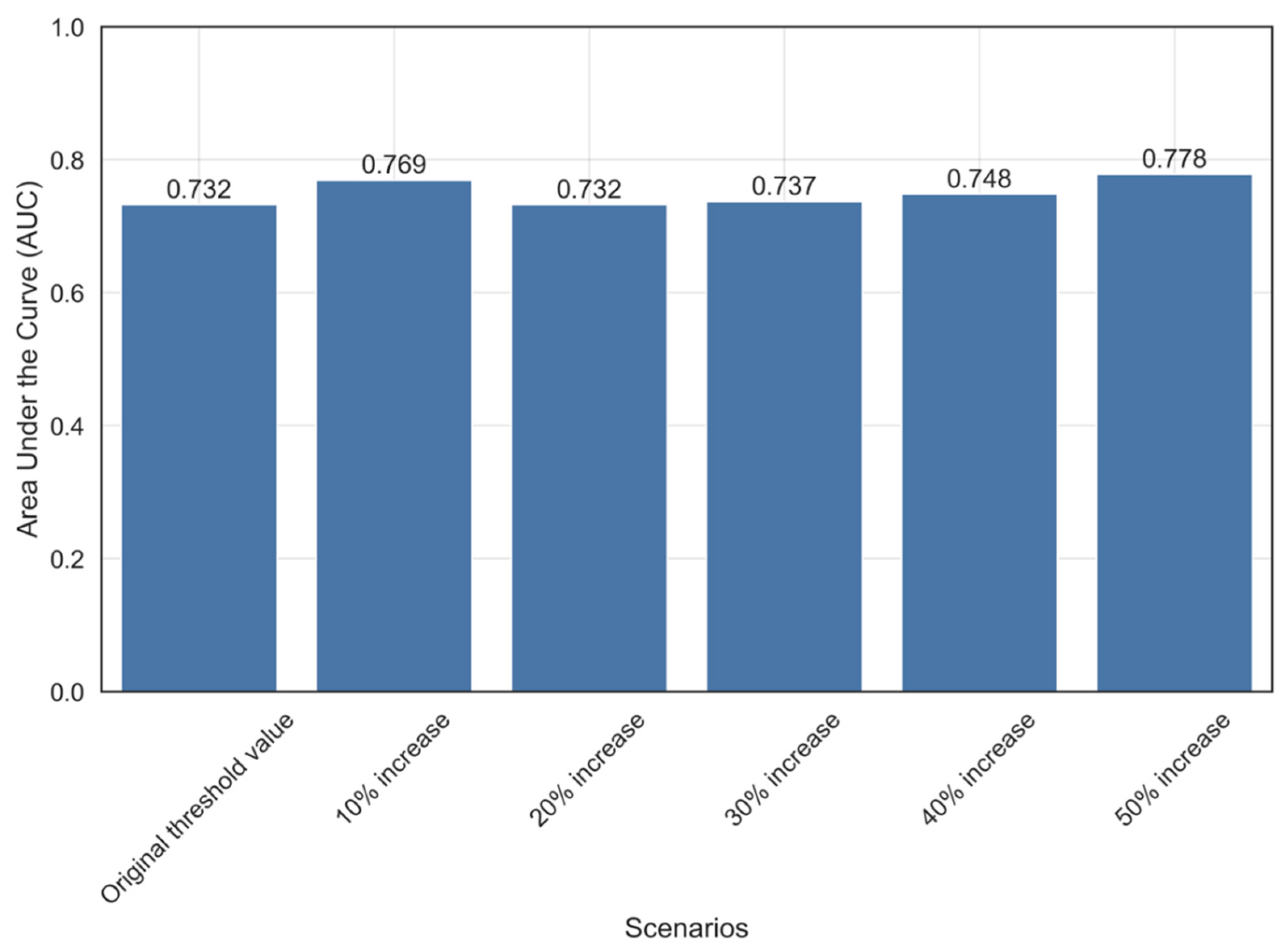
5. Results and Discussion

Table 3. Pavement Structural Condition Prediction Results Using Random Forest.

Predicted Class		True Class		Accuracy	Sensitivity/ Recall	Precision	F1-Score
		Poor Structural Condition	Non-Poor Structural Condition
	Poor Structural Condition	82	47	0.65	0.68	0.64	0.66
	Non-poor Structural Condition	39	77

,

Table 4. Pavement Structural Condition Prediction Results using XGBoost.

Predicted Class		True Class		Accuracy	Sensitivity/ Recall	Precision	F1-Score
		Poor Structural Condition	Non-Poor Structural Condition
	Poor Structural Condition	91	45	0.69	0.75	0.67	0.71
	Non-poor Structural Condition	30	79

and

Table 5. Pavement Structural Condition Prediction Results using Logistic Regression.

Predicted Class		True Class		Accuracy	Sensitivity/ Recall	Precision	F1-Score
		Poor Structural Condition	Non-Poor Structural Condition
	Poor Structural Condition	90	74	0.57	0.74	0.55	0.63
	Non-poor Structural Condition	31	50

show the prediction accuracy results obtained from the RF, XGBoost, and logistic regression models when they are applied to the test data set. The overall pavement structural condition prediction accuracy of the RF, XGBoost, and logistic regression models are 65%, 69%, and 57%, respectively. Thus, both machine learning models outperformed logistic regression. The XGBoost model had a higher sensitivity (75%) than the RF model (68%), indicating that it correctly predicted poor pavement condition for 75% of the segments and misclassified for 25%. In contrast, the RF model accurately predicted pavement condition for 68% of the segments and misclassified for 22%. The XGBoost model also outperformed the RF model in terms precision and F1-score. In terms of AUC, their values for RF, XGBoost, and logistic regression models are 0.718, 0.732, and 0.658, respectively. These results suggest that all three models yield moderately accurate predictions, with XGBoost being the best among the three for the data set used in this study.

The logistic regression model indicated that all three explanatory variables are statistically significant at the 90% confidence level. The XGBoost and RF models, on the other hand, do not report t-statistics for the variables. Instead, an importance value is reported, which are shown in

Table 6. Variable Importance Score obtained from RF and XGBoost model.

Model	Variable	Importance Value
RF	AADT	100
	Truck Percentage	77.7
	Speed limit	0
XGBoost	AADT	100
	Truck Percentage	58.94
	Speed limit	0

. As shown, the top two variables that affect a pavement’s structural condition are AADT and truck percentage, with AADT having higher importance. Both RF and XGBoost models indicated that speed limit has no effect or explanatory power on a pavement’s structural condition. A possible explanation for this finding is that, although slower speeds may have an effect on a pavement’s functional condition (Mshali and Steyn [32]), they do not necessarily have an effect on a pavement’s structural condition.

To determine the robustness of the XGBoost model, the SCI₁₂ threshold for poor structural condition was increased (from 3.3) by 10%, 20%, 30%, 40%, and 50%. The overall prediction accuracy and AUC of the XGBoost model are shown in Figure 8 and Figure 9, respectively. It can be seen that the prediction accuracy remains the same for all cases, except for the 50% case where it improved to 0.76 from 0.69. For AUC, the values fluctuate a bit from case to case, but overall, it remained in a tight range between 0.732 and 0.778. It can be concluded from this analysis that the threshold that divides the dataset into poor and non-poor segments had no effect on the predictive power of the XGBoost model.

6. Summary and Conclusions

This paper developed two machine learning models, eXtreme Gradient Boosting (XGBoost) and Random Forest (RF), to predict a pavement’s structural condition with the following explanatory variables: AADT, truck percentage, and speed limit. When the trained models were applied to the test data set, the results indicated that XGBoost and RF outperformed the logistic regression by 12% and 8%, respectively. The prediction accuracy of the XGBoost model was 4% higher than that of the RF model. Both XGBoost and RF models indicated that AADT and truck percentage have an effect on the pavement’s structural condition, whereas speed limit has no effect; the effect of AADT is higher than that of truck percentage. The prediction accuracy of the XGBoost model is robust when it was tested with different threshold values that divided the dataset into poor and non-poor pavement segments.

This study showed the potential of using machine learning to predict a pavement’s structural condition with readily available traffic data. A limitation of this study that should be kept in mind when applying the finding is that it considered a very limited set of contributing factors. The performance of XGBoost and RF may differ in another data set with more categories for the response variable and additional contributing factors. To overcome this shortcoming and to make the finding more generalizable, several areas will need to be improved upon. First, future work should utilize TSD data from a number of states located throughout the U.S. Second, additional variables, such as soil type, temperature, and pavement age, should be explored. Third, additional machine learning approaches should be investigated to identify the most suitable one(s). Lastly, the effectiveness of methods such as Bayesian techniques to deal with imbalanced data should be assessed.

References

1. Shrestha, S.; Katicha, S.W.; Flintsch, G.W. Application of Traffic Speed Deflectometer for Network-Level Pavement Management. Transp. Res. Rec. J. Transp. Res. Board 2018, 2672, 348–359. [Google Scholar] [CrossRef]
2. Flora, W.F. Development of a Structural Index for Pavement Management: An Exploratory Analysis. Master’s Thesis, Purdue University, West Lafayette, IN, USA, 2009. [Google Scholar]
3. Bryce, J.; Flintsch, G.; Katicha, S.; Diefenderfer, B. Developing A Network-Level Structural Capacity Index for Asphalt Pavements. J. Transp. Eng. 2013, 139, 123–129. [Google Scholar] [CrossRef]
4. Zaghloul, S.; He, Z.; Vitillo, N.; Kerr, J. Project Scoping Using Falling Weight Deflectometer Testing: New Jersey Experience. Transp. Res. Rec. J. Transp. Res. Board 1998, 1643, 34–43. [Google Scholar] [CrossRef]
5. Ferne, B.; Langdale, P.; Wright, M.; Fairclough, R.; Sinhal, R. Developing and Implementing Traffic-Speed Network Level Structural Condition Pavement Surveys. In Proceedings of the 9th International Conference on the Bearing Capacity of Roads, Railways and Airfields, Trondheim, Norway, 25–27 June 2013. [Google Scholar]
6. Steele, A.D.; Beckemeyer, C.A.; Van, T.P. Optimizing Highway Funds by Integrating RWD Data into Pavement Management Decision Making. In Proceedings of the 9th International Conference on Managing Pavement Assets, Washington, DC, USA, 18–21 May 2015. [Google Scholar]
7. Katicha, W.S.; Ercisli, S.; Flintsch, G.W.; Bryce, J.M.; Diefenderfer, B.K. Development of Enhanced Pavement Deterioration Curves; VTRC 17-R7; Virginia Transportation Research Council: Charlottesville, VA, USA, 2016. [Google Scholar]
8. Nasimifar, M.; Thyagarajan, S.; Chaudhari, S.; Sivaneswaran, N. Pavement Structural Capacity from Traffic Speed Deflectometer for Network Level Pavement Management System Application. Transp. Res. Rec. J. Transp. Res. Board 2019, 2673, 456–465. [Google Scholar] [CrossRef]
9. Manoharan, S.; Chai, G.; Chowdhury, S. A Study of The Structural Performance of Flexible Pavements Using Traffic Speed Deflectometer. J. Test. Eval. 2018, 46, 1280–1289. [Google Scholar] [CrossRef] [Green Version]
10. Chai, G.; Manoharan, S.; Golding, A.; Kelly, G.; Chowdhury, S. Evaluation of the Traffic Speed Deflectometer Data using Simplified Deflection Model. Transp. Res. Procedia 2016, 14, 3031–3039. [Google Scholar] [CrossRef] [Green Version]
11. Shrestha, S.; Katicha, S.W.; Flintsch, G.W. Development of Traffic Speed Deflectometer Structural Condition Thresholds Based on Pavement Management Condition Data. In Proceedings of the 98th Annual Meeting of the Transportation Research Board, Washington, DC, USA, 12–16 January 2018. [Google Scholar]
12. Manoharan, S.; Chai, G.; Chowdhury, S. Structural Capacity Assessment of Queensland Roads Using Traffic Speed Deflectometer Data. Aust. J. Civ. Eng. 2020, 18, 219–230. [Google Scholar] [CrossRef]
13. Zihan, A.U.; Elseifi, M.A.; Gaspard, K.; Zhang, Z. Development of Structural Capacity Prediction Model Based on Traffic Speed Deflectometer Measurements. Transp. Res. Rec. J. Transp. Res. Board 2018, 2672, 315–325. [Google Scholar] [CrossRef]
14. Zhang, Y.; Haghani, A. A Gradient Boosting Method to Improve Travel Time Prediction. Transp. Res. Part C Emerg. Technol. 2015, 58, 308–324. [Google Scholar] [CrossRef]
15. Kim, J.E.; Park, H.C.; Ham, S.W.; Kho, S.Y.; Kim, D.K. Extracting Vehicle Trajectories Using Unmanned Aerial Vehicles in Congested Traffic Conditions. J. Adv. Transp. 2019, 2019, 9060797. [Google Scholar] [CrossRef]
16. Luo, X.; Li, D.; Yang, Y.; Zhang, S. Spatiotemporal Traffic Flow Prediction with KNN and LSTM. J. Adv. Transp. 2019, 2019, 4145353. [Google Scholar] [CrossRef] [Green Version]
17. Eraqi, M.H.; Abouelnaga, Y.; Saad, M.H.; Moustafa, M.N. Driver Distraction Identification with an Ensemble Of Convolution Neural Networks. J. Adv. Transp. 2019, 2019, 4125865. [Google Scholar] [CrossRef]
18. Xue, Q.; Wang, K.; Lu, J.J.; Liu, Y. Rapid Driving Style Recognition in Car-Following Using Machine Learning and Vehicle Trajectory Data. J. Adv. Transp. 2019, 2019, 9085238. [Google Scholar] [CrossRef] [Green Version]
19. Shang, Q.; Tan, D.; Gao, S.; Feng, L. A Hybrid Method for Traffic Incident Duration Prediction Using Boa-Optimized Random Forest Combined With Neighborhood Components Analysis. J. Adv. Transp. 2019, 2019, 4202735. [Google Scholar] [CrossRef] [Green Version]
20. Sun, S.; Zhang, J.; Bi, J.; Wang, Y. A Machine Learning Method for Driving Range of Battery Electric Vehicles. J. Adv. Transp. 2019, 2019, 4109148. [Google Scholar] [CrossRef]
21. Cheng, Y.; Chen, X.; Ding, X.; Zeng, L. Optimizing Location of Car-Sharing Stations Based On Potential Travel Demand And Present Operation Characteristic: The Case of Chengdu. J. Adv. Transp. 2019, 2019, 7546303. [Google Scholar] [CrossRef] [Green Version]
22. Abdelaziz, N.; El-Hakim, R.T.A.; El-Badawy, S.M.; Afify, H.A. International Roughness Index prediction model for flexible pavements. Int. J. Pavement Eng. 2020, 21, 88–99. [Google Scholar] [CrossRef]
23. Kaloop, R.M.; El-Badawy, S.M.; Ahn, J.; Sim, H.-B.; Hu, J.W.; El-Hakim, R.T.A. A Hybrid Wavelet-Optimally-Pruned Extreme Learning Machine Model for the Estimation of International Roughness Index Of Rigid Pavements. Int. J. Pavement Eng. 2022, 23, 862–876. [Google Scholar] [CrossRef]
24. Guo, R.; Fu, D.; Sollazzo, G. An Ensemble Learning Model for Asphalt Pavement Performance Prediction Based on Gradient Boosting Decision Tree. Int. J. Pavement Eng. 2021; ahead-of-print. [Google Scholar] [CrossRef]
25. Karballaeezadeh, N.; Tehrani, H.G.; Shadmehri, D.M.; Shamshirband, S. Estimation Of Flexible Pavement Structural Capacity Using Machine Learning Techniques. Front. Struct. Civ. Eng. 2020, 14, 1083–1096. [Google Scholar] [CrossRef]
26. Justo-Silva, R.; Ferreira, A.; Flintsch, G. Review on Machine Learning Techniques for Developing Pavement Performance Prediction Models. Sustainability 2021, 13, 5248. [Google Scholar] [CrossRef]
27. Rahman, M.M.; Uddin, M.M.; Gassman, S.L. Pavement Performance Evaluation Model for South Carolina. KSCE J. Civ. Eng. 2017, 21, 2695–2706. [Google Scholar] [CrossRef]
28. Kim, S.; Kim, N. Development of Performance Prediction Models in Flexible Pavement Using Regression Analysis Method. KSCE J. Civ. Eng. 2017, 10, 91–96. [Google Scholar] [CrossRef]
29. Qu, L.; Zhang, Y.; Harvey, J.T. Estimation of Truck Traffic Inputs for Mechanistic -Empirical Pavement Design in California. Transp. Res. Rec. J. Transp. Res. Board 2009, 2095, 62–72. [Google Scholar]
30. Chou, C.P.J. Effect of Overloaded Heavy Vehicles On Pavement and Bridge Design. Transp. Res. Rec. J. Transp. Res. Board 1996, 1539, 58–65. [Google Scholar] [CrossRef]
31. Salama, K.H.; Chatti, K.; Lyles, R.W. Effect of Heavy Multiple Axle Trucks on Flexible Pavement Damage Using In-Service Pavement Performance Data. J. Transp. Eng. 2006, 132, 763–770. [Google Scholar] [CrossRef] [Green Version]
32. Mshali, R.M.; Steyn, W.J. Effect of Truck Speed on The Response of Flexible Pavement Systems to Traffic Loading. Int. J. Pavement Eng. 2020, 23, 1213–1225. [Google Scholar] [CrossRef]
33. Jiang, X.; Abdel-Aty, M.; Hu, J.; Lee, J. Investigation Macro-Level Hotzone Identification and Variable Importance Using Big Data. Neurocomputing 2016, 181, 53–63. [Google Scholar] [CrossRef]
34. Gong, H.; Sun, Y.; Huang, B. Gradient Boosted Models for Enhancing Fatigue Cracking Prediction In Mechanistic-Empirical Pavement Design Guide. J. Transp. Eng. Part B Pavements 2019, 145, 04019014. [Google Scholar] [CrossRef]
35. Rezapour, M.; Molan, A.M.; Ksaibati, K. Analyzing Injury Severity of Motorcycle At-Fault Crashes Using Machine Learning Techniques, Decision Tree And Logistic Regression Models. Int. J. Transp. Sci. Technol. 2020, 9, 89–99. [Google Scholar] [CrossRef]
36. Biau, G.; Scornet, E. A Random Forest Guided Tour. TEST 2016, 25, 197–227. [Google Scholar] [CrossRef] [Green Version]
37. Chen, T.; Guestrin, C. XGBoost: A Scalable Tree Boosting System. In Proceedings of the 22nd ACM SIGKDD International Conference on Knowledge Discovery and Data Mining, San Francisco, CA, USA, 13–17 August 2016. [Google Scholar]
38. Li, J.; An, X.; Li, Q.; Wang, C.; Yu, H.; Zhou, X.; Geng, Y. Application of XGBoost Algorithm in the Optimization of Pollutant concentration. Atmos. Res. 2022, 276, 106238. [Google Scholar] [CrossRef]
39. McDowell, I. Measuring Health: A Guide to Rating Scales and Questionnaires; Oxford University Press: Oxford, UK, 2006. [Google Scholar]
Figure 1. Primary routes selected by SCDOT to have TSD data collected.
Sustainability 14 08627 g001
Figure 2. iPAVe used to collect pavement condition data in South Carolina (source: https://www.arrb.com.au/ipave accessed on 13 July 2022).
Sustainability 14 08627 g002
Figure 3. Percentages of segments with poor and non-poor structural condition for each route.
Sustainability 14 08627 g003
Figure 4. Boxplots of segments’ AADTs for each route.
Sustainability 14 08627 g004
Figure 5. Boxplots of segments’ truck percentages for each route.
Sustainability 14 08627 g005
Figure 6. Boxplots of segments’ speed limits for each route.
Sustainability 14 08627 g006
Figure 7. Distribution of segments’ SCI12 values for each route.
Sustainability 14 08627 g007aSustainability 14 08627 g007b
Figure 8. Overall prediction accuracy of the XGBoost model at different SCI12 threshold values.
Sustainability 14 08627 g008
Figure 9. AUC of the XGBoost model at different SCI12 threshold values.
Sustainability 14 08627 g009