Article

How Does Retailer-Oriented Remanufacturing Affect the OEM’s Quality Choice?

1
Business School, Shantou University, Shantou 515063, China
2
School of Maritime Economics and Management, Dalian Maritime University, Dalian 116026, China
3
School of Economics and Management, Dalian University of Technology, Dalian 116023, China
*
Author to whom correspondence should be addressed.
Sustainability 2022, 14(13), 8028; https://doi.org/10.3390/su14138028
Submission received: 27 May 2022 / Revised: 19 June 2022 / Accepted: 27 June 2022 / Published: 30 June 2022
(This article belongs to the Section Waste and Recycling)

Abstract

:
We consider that a supply chain consists of an original equipment manufacturer (OEM) and a retailer. We analyze how the retailer’s remanufacturing decision affects the decision of the new products’ qualities for the OEM. We use a game theory approach to investigate the interactions between the OEM and the retailer with or without remanufacturing operation. We find the retailer’s motivation to develop the remanufacturing industry depends on the profitability of remanufactured products and the OEM’s deterring strategy. When the remanufacturing operation profit margin is low, the retailer voluntarily gives up remanufacturing; when this profit margin is moderate, the OEM induces the retailer to give up remanufacturing by improving the quality of the new product; when this profit margin is sufficiently high, the OEM cannot prevent the retailer from developing remanufacturing. The retailer developing remanufacturing as well as their threat of developing decrease the OEM’s profit because the OEM improves the quality of the new products to induce the retailer to give up remanufacturing, at the expense of its own profit. We explicitly characterize the process of the OEM from preventing to accepting the retailer developing the remanufacturing industry, as well as the changes in supply-chain members’ operating decisions and profits in the process. Finally, using MATLAB numerical analysis, we also found that the retailer’s development of the remanufacturing industry always benefits the whole supply chain, consumer surplus, and social welfare. Furthermore, the retailer’s development of the remanufacturing industry is not always good for the environment. This development is only good for the environment when the new products’ environmental impacts in the EOL stage are larger than the total environmental impacts of the remanufactured products in every stage of their life cycle.

1. Introduction

The economy’s development and the improvement of science and technology accelerate the replacement of various products. As a result, a large number of waste products that may contain some toxic substances are emerging. The living environment of humans is deteriorating rapidly and facing the pressure of pollution products. Countries worldwide pay more attention to products’ environmental performance, and sustainable manufacturing and service operations are gaining increasing recognition [1]. Every country or region is looking for sustainable production methods, among which remanufacturing is one of the most efficient so far [2].
Remanufacturing involves taking end-of-life (EOL) products and bringing them back to an as-new condition and reselling them [3]. Remanufacturing is perceived as an environmentally friendly initiative for eliminating the impact of returned core disposal. Compared to the production of new products, only about 15% of the original resources are required in remanufacturing [4]. Therefore, a number of governments support remanufacturing actively. Many countries and regions have enacted legislation such as the Waste Electrical and Electronic Equipment (WEEE) in Europe, the End-of-Life Vehicles Directive (ELV Directive) in the European Union, and the Home Appliance Recycling Law in Japan. The Chinese government also acknowledges environmental problems caused by end-of-life products and has enacted a series of laws and legislation, including the Trade Old for Remanufactured Program, Circular Economy Promotion Law, and Recommendations on Promoting Remanufacturing Industry [5]. These pieces of legislation encourage firms to develop remanufacturing operations by providing assistance to those firms. In fact, remanufacturing attracts more and more corporations such as HP, IBM, Apple, BMW, Xerox, Caterpillar, and Cannon to participate to pursue the economic benefits. This study shows remanufacturing could save 40–65% of the cost of traditional manufacturing [4]. The average profit margins from remanufacturing can exceed 20% [6]. The Xerox Corporation, for instance, has earned nearly USD 200 million by remanufacturing the recovered copier [7].
Despite the huge benefits of remanufacturing operations, many original equipment manufacturers (OEMs) give up developing remanufacturing due to its challenges. OEMs may confront three main challenges when developing remanufacturing. First, market cannibalization by remanufactured products is a major concern for many OEMs [3]. Assessment of market cannibalization of remanufacturing is also an important issue in operations management and industrial ecology [8]. Second, even if cannibalization is not a concern, the OEMs may still experience challenges from the specialized knowledge or technology in production, which requires adopting different manufacturing techniques. Third, because the process of remanufacturing is different from that of new product production, with differences including the collection of cores and the demand for remanufactured products, it is also necessary to master related management skills. Therefore, many OEMs have no incentive to involve themselves in remanufacturing. In practice, the majority of remanufacturing activities have been carried out by many independent remanufacturers [9].
Among those remanufacturers, there is no lack of retailers or firms employed by retailers. For example, SEVALO Construction Machinery Group Corporation is the main distributor of the Doosan Infracore Corporate in China. Namely, SEVALO retails excavators produced by Doosan. Moreover, SEVALO also remanufactures the EOL or end-of-use excavators produced by Doosan [10]. Recently, we find big retailers also developing remanufacturing; examples include Walmart, Amazon, and BestBuy, which not only sell new products but also participate in recycling and selling remanufactured products, such as smartphones.
In this paper, we develop a game-theoretical model to analyze the effect of retailer-oriented remanufacturing on OEM’s quality choice of new products. Following [11], we assume that the quality of a remanufactured product is also determined by the quality of new ones because EOL or end-of-use products are the raw materials of remanufacturing. We analyze the interactivity between the upstream (the OEM) and the downstream (the retailer). Several researchers have already studied the issue of remanufacturing’s effect on new products’ qualities. However, most studies mainly focus on the effect of independent remanufacturer-oriented remanufacturing on the OEM’s quality choice of the new product [11], or the OEM’s itself-oriented remanufacturing on the quality choice of the new product [12]. Nevertheless, retailer-oriented remanufacturing is also prevalent, as stated above. Retailers engaging in remanufacturing will change the relationship with the OEM from cooperation to coopetition. We are concerned about the effect of coopetition on the decisions of the OEM and the retailer. As far as we know, only a few scholars discuss the form in which retailers undertake remanufacturing [13], but they do not consider the quality difference between the new and remanufactured products.
The concerns of this paper are as follows: First, does the retailer have the motivation to develop the remanufacturing operation? Second, what is the impact on the supply-chain operation and relationship with the OEM if the retailer engages in remanufacturing? Third, how does the OEM deal with the cannibalization problem, and will the quality of the new product deteriorate? Last, what environmental and social welfare changes will this form of remanufacturing bring?
The remainder of this paper is organized as follows: Section 2 provides a related literature review. Section 3 describes the model and equilibrium results. Section 4 studies the impact of retailers’ remanufacturing on products’ qualities, customer surplus, social welfare, and the environment. We conclude the results and give some managerial implications in Section 5. All the proofs are provided in Appendix A.

2. Literature

This study mainly relates to three streams of literature: remanufacturing supply-chain management, the environmental impact of remanufacturing, and the quality decision in supply-chain operation.

2.1. Remanufacturing Supply-Chain Management

The remanufacturing strategy has received great attention for its business benefits [7,14]. Previous researchers mainly focused on the conditions of the remanufacturing strategy and the operational forms of the remanufacturing supply chain. Atasu et al. (2008) obtained the thresholds on the remanufacturing cost savings, green segment size, market growth rate, and consumer valuations for the remanufactured products above, the remanufacturing of which made profits under the monopolistic and competitive conditions [15]. Chen and Chang (2012) explored the remanufacturing strategy under the cooperative and competitive setting to investigate the conditions in which the OEM should participate in remanufacturing or permit a third-party firm to remanufacture the products. They found the choice of remanufacturing depends on the costs of remanufacturing and the competition intensity of the new and remanufactured products [16]. Zou et al. (2016) discussed the decisions between outsourcing or authorization of the OEM on allowing the third-party remanufacturer (3PR) to perform remanufacturing operations. They found the OEM always prefers outsourcing, and the 3PR’s approach preference depends on consumers’ perceived value of the remanufactured products [17]. Qian et al. (2020) discussed the remanufacturing form in which OEMs should outsource their remanufacturing operations to their retailers. Their results demonstrated that although outsourcing remanufacturing is beneficial to retailers, it always hurts OEMs and the remanufacturing industry [13]. Some scholars have also discussed the impact of the key procedure in remanufacturing. For example, Savaskan et al. (2004) addressed the problem of the collection channel structure choice in the remanufacturing strategy. They considered three options for the manufacturer including collecting by itself directly from the customers, inducing the retailer to collect, and subcontracting the collection activity to a third party. The results show that the retailer’s collection mode is most effective [18].
Recent research also paid attention to the operation decisions in the specific remanufacturing mode. Abbey et al. (2015) discussed the pricing decision of the remanufacturing supply chain. They found that the optimal price of the new product should increase when the remanufactured products enter. In addition, the OEM adopting appropriate pricing of the new products can mitigate the effects of cannibalization and increase profit [19]. Örsdemir et al. (2014) investigated the quality decision of new products in the remanufacturing supply chain with an OEM and independent remanufacturer competing with each other. The results showed that the OEM relies more on quality as an effective competitive tool when it has a stronger competitive position, while it relies more on limiting the recovery amount of cores when its competitive position is weaker [11]. Jena and Sarmah (2016) studied price and service coopetition between two remanufacturing firms considering uncertain demand. They developed four different remanufacturing configurations and derived the corresponding equilibrium decision [20]. Chen et al. (2020), using the evolutionary game model, analyzed the interaction between the government and the enterprises, and found that regulation exerts significant influences on enterprises’ remanufacturing operation decisions [21]. Many other scholars have considered the influence of other factors on the operation decision of the remanufacturing supply chain such as channel structure and governments’ subsidy policies [22,23], different channel power structures [5], lost sales and uncertain quality [24], cost disruption [25], returns at different quality grades [26], warranty strategy [27], and collectors’ fairness concerns [28]. In contrast to their works, we contribute to retailer-oriented remanufacturing by investigating the interaction between the OEM and the retailer. We focus on the effect of retailer-oriented remanufacturing on the decisions of the quality and wholesale price of the new product for the OEM.

2.2. Environmental Impact of Remanufacturing

Business benefits, environmental concerns, and environmental regulations promote the development of remanufacturing [29,30,31,32]. Neto and Bloemhof (2012) examined the eco-efficiency of remanufacturing in the personal-computer and mobile-phone industries. They found remanufacturing is an effective way to reduce the total energy consumed during the life cycles of personal computers and mobile phones, except for the life spans of remanufactured products, which are remarkably shorter than those of their new counterparts [33]. Yenipazarli (2016) discussed the role of emissions regulations in remanufacturing’s environmental impact. The results showed that when the emissions charge is low, remanufacturing could reduce total emission but could not achieve a “win–win” result for the OEM and remanufacturer. When the emissions charge is high, remanufacturing could bring a negative environmental effect but a “win–win” economic benefit [32]. He et al. (2019) found that a higher subsidy level always benefits consumers and the whole supply chain but does not always benefit the environment. Only when the environmental impact discount of remanufactured products satisfies certain conditions can the government subsidy improve the environment [23]. Yan et al. (2015) investigated two channel structures of marketing remanufactured products; one is marketing through the manufacturer’s own e-channel and the other is marketing through a third party. The results showed that the first channel structure is always better for the environment, but the manufacturer has no incentive to adopt it due to the benefits [31]. Gu et al. (2015) found that the effects of consumer preferences and production technology on profit were consistent with those effects on environmental friendliness only when such effects are manifested through remanufactured products rather than through new products [34]. Ovchinnikov et al. (2014) provided a data-driven economic and environmental assessment of remanufacturing for product and service firms. The results showed that remanufacturing is often consistent with firms’ economic and environmental goals for increasing profits and decreasing environmental impact [8]. In addition, some scholars used empirical or case methods to conduct corresponding studies on different industries in different regions, such as industries of Thailand [35], and Fuji Xerox in Australia [36]. Although these studies concern the environmental impact of remanufacturing, they do not discuss the situation when the retailer works out remanufacturing operations.

2.3. Quality Decision in Supply-Chain Operation

This paper is closely related to the literature rooted in the quality decision of supply-chain operations. Products’ demands closely relate to their qualities [37,38], and the quality-decision problem in the supply chain attracts much attention from many scholars. Xie et al. (2011) explored quality investment and the pricing decision of a make-to-order (MTO) supply chain with uncertain demand. They demonstrated that quality investment and pricing were significantly affected by both supply-chain strategy and risk-averse behavior [39]. Ma et al. (2013) compared three different supply-chain structures in a two-stage supply chain and pointed out the manufacturer’s and retailer’s preferred supply-chain structures [40]. Hsieh and Liu (2010) investigated the supplier’s and manufacturer’s quality investment and inspection strategies in four noncooperative scenarios, and they obtained the equilibrium investment amount and equilibrium profit in different scenarios [41]. Veldman and Gaalman (2014) considered two owner–manager pairs in competition and investigated the effects of strategic incentives for product quality. They found only one firm owner can instruct his or her manager to maximize a nonprofit function in the asymmetric case; however, both firm owners can set product quality incentive weights to obtain higher product quality levels in the symmetric case [42]. Liu et al. (2018) investigated the timing issue of sales commitment in a supply chain with manufacturer-quality and retailer-effort induced demand. They found that delay commitment could increase both the manufacturer’s and retailer’s investment levels and the manufacturer prefers delayed commitment when the quality enhancement variability is high enough [43]. Liu et al. (2014) determined a joint dynamic pricing and preservation technology investment strategy in a food supply chain [44]. Atasu and Souza (2013) studied the impact of product recovery on a firm’s product quality choice. They found three main factors play an important role in quality choice, namely the form of product recovery, recovery cost structure, and the presence of product take-back legislation [12]. Differently, our study concerns how downstream retailers’ remanufacturing operations affect the OEM’s quality choice of the new products. There are special characteristics in this supply chain in our work, such as the cooperation between the OEM and the retailer.

3. Model and Equilibrium Results

3.1. Model Description

In this paper, we consider a supply-chain structure with a downstream retailer (denoted by R) and an upstream original equipment manufacturer (denoted by OEM). First, we discuss a basic model in which the retailer only resells the new products and does not remanufacture the EOL products, and the OEM designs the qualities of new products and sells products to the retailer. For convenience, we denote the basic model as Case NR. Then, we consider the model in which the retailer develops the remanufacturing operations and resells both new and remanufactured units to the customer. Facing the threat of the remanufactured products cannibalizing the market share of the new products, the OEM changes the wholesale prices and qualities of the new products. We denote the second model as Case R. Figure 1 illustrates the supply chain structures of the two operation modes.
We summarize the key notations in Table 1.

3.1.1. Customer Choice Behavior

We model customer choice behavior in the same way as Örsdemir et al. (2014) [11]. We assume the potential market size is normalized to 1 in each model. We denote a customer’s willingness to pay for a new product’s quality level s as s v , where v is distributed uniformly over [ 0 , 1 ] . A customer with willingness to pay s v for a new product also has willingness to pay δ s ν for a remanufactured product where δ 0 , 1 . Subramanian and Subramanyam (2015) found that customers often perceive the new product as being of superior quality [30]. We represent this factor by modeling a differentiation between customers’ willingness to pay for the new product and remanufactured product. If the prices of the new and remanufactured units are p N and p R , respectively, a customer with willingness to pay v will derive net utility U N = s v p N to buy a new product and derive net utility U R = δ s v p R to buy a remanufactured unit. Obviously, as long as v p N / s , the customer with willingness to pay v finds the new product acceptable, and as long as v p R / δ s , the customer finds the remanufactured product acceptable. Therefore, when only new products are sold in the market, a customer with willingness to pay v p N / s will buy the new product. However, when both the new and remanufactured units are sold simultaneously, a customer with willingness to pay s v p N max δ s v p R , 0 will buy the new product, a customer with willingness to pay δ s v p R max s v p N , 0 will buy the remanufactured unit, and a customer with willingness to pay s v p N < 0 and δ s v p R < 0 will buy nothing.

3.1.2. Demand Functions

Based on the above customer-choice behavior analysis, we can derive the demand functions of the new and remanufactured products. In model NR, there are no remanufactured products, so customers with willingness to pay v p N / s , 1 will buy the products. In model R, there are new products and remanufactured products simultaneously, so customers with willingness to pay v p N p R / s 1 δ , 1 prefer to buy a new product and those with willingness to pay v p R / δ s , p N p R / s 1 δ will buy the remanufactured products. Because v is distributed uniformly over [ 0 , 1 ] , the demand for the new products in model NR is
Q N - NR = p N / s 1 f v d v = 1 p N s
and the demands for the new products and remanufactured products in model R are
Q N - R = p N p R / s 1 δ 1 f v d v = 1 p N p R s 1 δ
Q R - R = p R / δ s p N p R / s 1 δ f v d v = p N p R s 1 δ p R s δ
where f v is the probability density function of v . They lead to the inverse demand functions via a simple algebraic operation as follows:
p N = s 1 Q N δ Q R
p R = s δ 1 Q N Q R

3.1.3. Cost Functions

Similar to Örsdemir et al. (2014) [11] and Atasu and Souza (2013) [12], we assume the unit variable cost of manufacturing a new product with quality level s is β s 2 , where β is the scaling parameter. Because remanufactured products reuse some parts of the EOL product and replace the worn-out parts (i.e., changing the quality), the unit variable cost of the remanufactured product is less than that of the new product. Specifically, following Örsdemir et al. (2014) [11], the remanufactured product’s unit variable cost is proportional to that of the new product (i.e., α β s 2 , where α 0 , 1 indicates the variable cost advantage of the remanufactured product compared to the new product).

3.2. Model and Equilibrium Result

We consider a single-period model, which Subramanian et al. (2011) [30], Atasu and Souza (2013) [12], and Örsdemir et al. (2014) [11], for example, extensively used. A single-period model focuses on steady-state profits and facilitates analytical tractability, which allows us to focus on our research questions. In addition, all products’ useful lifetimes are one period, and they can be remanufactured only once, which is the same as in the work of Atasu and Souza (2013) [12] and Örsdemir et al. (2014) [11].

3.2.1. Basic Model without Remanufacturing (Model NR)

In model NR, the supplier first decides the quality level s of the products. Then, the supplier sets the wholesale price w of the new products and sells them to the retailer. After viewing the quality level s and wholesale price w , the retailer decides the order quantity Q N . In this setting, the supplier’s and retailer’s decision problems are, respectively, as follows:
Π OEM - NR = max s , w w β s 2 Q N
Π R - NR = max Q N s 1 Q N w Q N
We derive the equilibrium results using backward induction, and the equilibrium results are shown in Table 2. All the technical proofs are provided in Appendix A.

3.2.2. Retailer Developed Remanufacturing (Model R)

In model R, the retailer develops the remanufacturing operations. Facing the challenge from the retailer, the supplier will change the quality level s and wholesale price. In this setting, the sequence of events is as follows: first, the supplier decides the quality level s and wholesale price w of the new products. Given quality level s and wholesale price w , the retailer decides the order quantity of the new products Q N and the quantity of the remanufactured products Q R . In this setting, the supplier’s and retailer’s decision problems are, respectively, as follows:
Π OEM - R = max s , w w β s 2 Q N
Π R - R = max Q N , Q R s 1 Q N δ Q R w Q N + s δ 1 Q N Q R α β s 2 Q R
We still use backward induction to solve this dynamic game, and the equilibrium results are shown in Table 3.

4. Equilibrium Result Analysis

4.1. Operation Decision and Profits

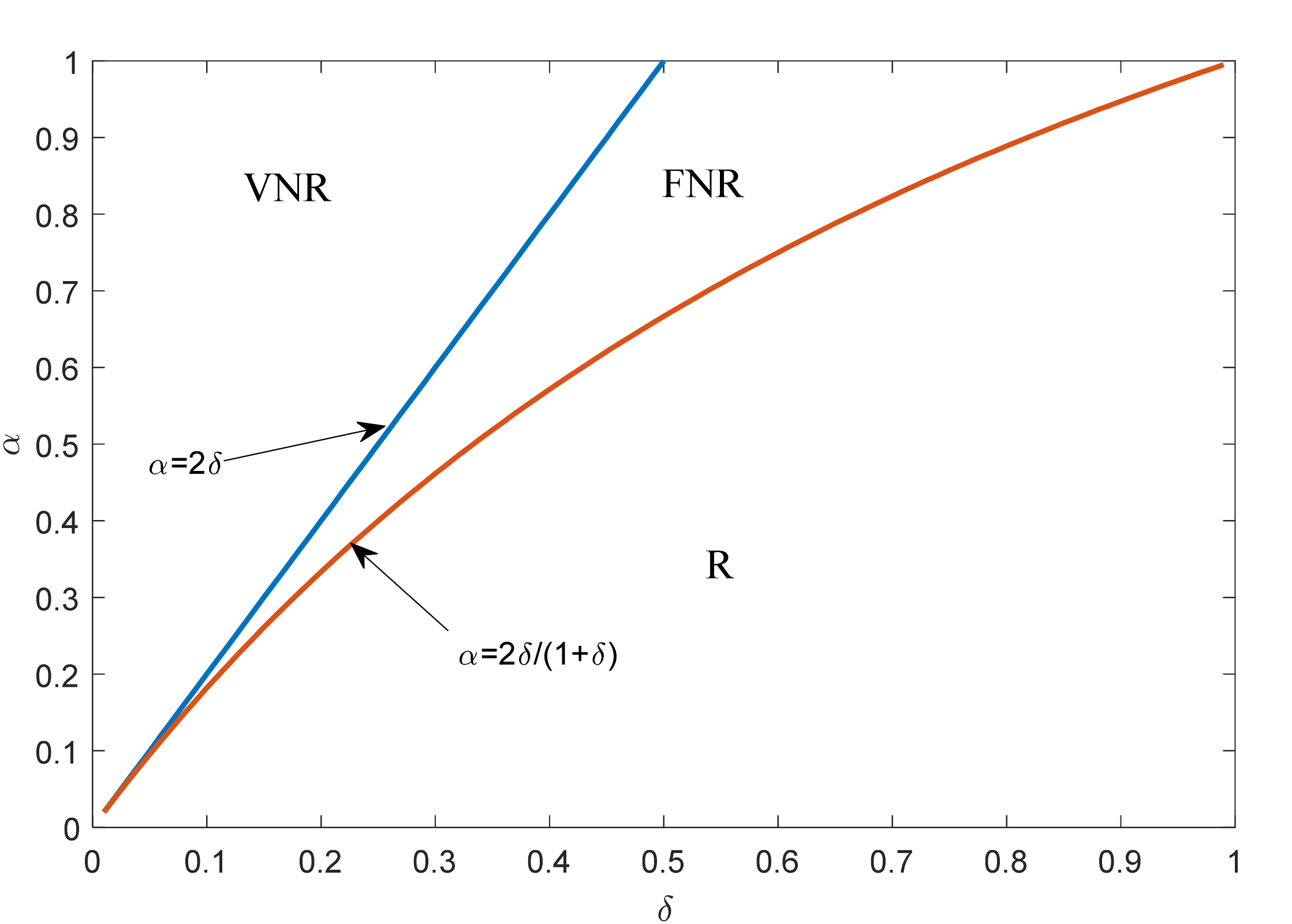
In this section, we discuss the operation decisions and profits of the OEM and the retailer in equilibrium. Remanufactured products’ cost-to-value ratio α / δ , which could reflect the profitability of remanufactured products, is used as an important proportionality factor in this part of the discussion. Figure 2 graphically shows the equilibrium regions in model R. We take the value δ 0 , 1 and α 0 , 1 ; a larger δ indicates a higher consumer valuation of the remanufactured products, while a smaller α indicates a larger cost advantage of the remanufactured products over the new products. The value ranges in Figure 2 cover all the situations of retailers developing remanufacturing operations from the two dimensions of cost advantage and recognition of remanufactured products for customers. The retailer will choose different remanufactured strategies at different locations in this two-dimensional coordinate system. The boundary conditions α / δ 2 , 2 / 2 δ < α / δ < 2 , and α / δ < 2 / 2 δ in Table 3 correspond to the conditions under which the retailer voluntarily gives up remanufacturing, the retailer is forced to give up remanufacturing, and the retailer develops remanufacturing, respectively. By describing these three conditions in the above two-dimensional coordinate system, the retailer’s strategy choices under different cost-to-value ratios can be obtained, as shown in Figure 2.
Proposition 1.
If α / δ 2 , then the retailer voluntarily gives up the remanufacturing operations; if 2 / 2 δ < α / δ < 2 , the supplier deters the retailer from developing remanufacturing operations by improving the quality and dropping the wholesale price of the new products; if α / δ < 2 / 2 δ , the retailer develops the remanufacturing operations.
Figure 2 graphically depicts the equilibrium regions of the remanufacturing strategy, which we describe as Proposition 1. We can see the retailer will adopt different strategies according to the cost-to-value ratio. We divide the entire range into three regions according to the distribution of α and δ , namely region VNR, region FNR, and region R, wherein region VNR implies the retailer gives up remanufacturing voluntarily, region FNR implies the manufacturer forces the retailer to give up remanufacturing via strategy adjustment, and region R implies the retailer develops remanufacturing operations.
In region VNR, the retailer will not actively develop remanufacturing due to the cost-to-value ratio being high, which means the retailer must pay a high cost to obtain value from remanufacturing. The retailer voluntarily gives up the remanufacturing operations because remanufacturing does not generate profits in this situation.
In region FNR, the retailer has a motive but still does not develop remanufacturing, even if the cost-to-value ratio decreases and the profitability of remanufacturing is attractive in this region. That is because if the retailer develops remanufacturing, its profits come from two parts, new products and remanufactured products, so the retailer will trade off the profit of these two parts. At the same time, the relationship of the OEM and the retailer will also change from cooperative to coopetitive (competition exists together with cooperation). The OEM only obtains profits from new products; in this region, the OEM deters the retailer from developing remanufacturing operations by improving the quality and increasing the wholesale price of the new products to avoid cannibalization. On the one hand, this operation of the OEM will increase the cost of the retailer’s remanufacturing, for the remanufacturing cost is positively correlated with the cost of the new products. On the other hand, if the OEM increases the wholesale price, the margin profit of the new products decreases. Therefore, the retailer will give up the remanufacturing strategy after the trade-off.
In region R, the cost-to-value ratio is sufficiently low, which means remanufactured products have sufficient profitability, and the retailer will develop the remanufacturing industry and sell new and remanufactured products at the same time.
Proposition 2.
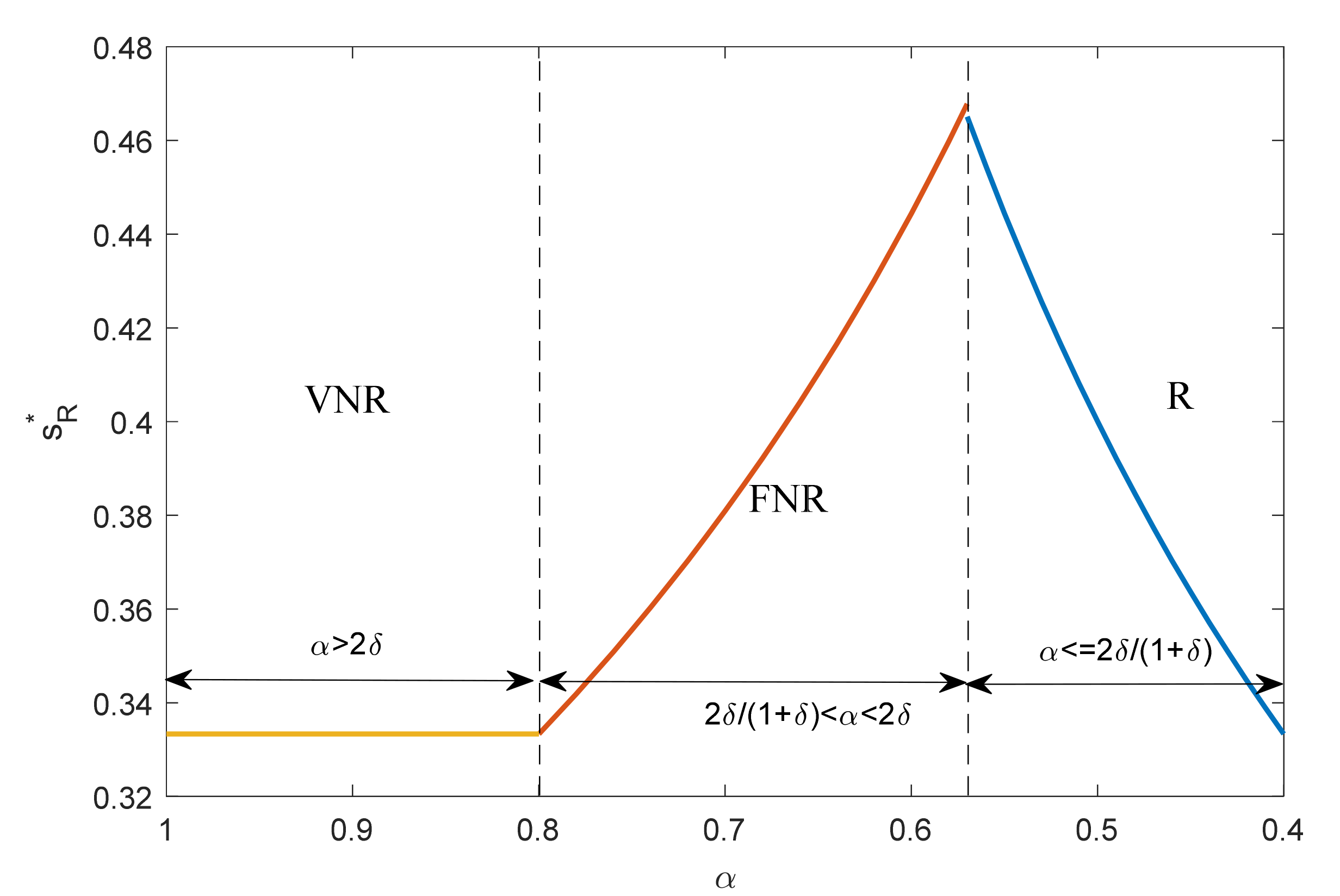
When α / δ 2 , s R * = s NR * ; when 2 / 1 + δ < α / δ < 2 , s R * > s NR * and s R * / α < 0 ; when 1 < α / δ < 2 / 1 + δ , s R * > s NR * , s R * / α > 0 , and lim α δ s R * = s NR * .
Figure 3 shows the change process of the new products’ qualities with respect to the cost-to-value ratios of the remanufactured products, which is described in Proposition 2. When α / δ 2 , the OEM will not change the new products’ qualities, for the retailer will not enter the remanufacturing market due to the high cost of remanufacturing and because the OEM has a monopoly in the market. When 2 / 1 + δ < α / δ < 2 , the OEM will improve the new products’ qualities to deter the retailer from entering the remanufacturing industry, and the new products’ qualities increase as α / δ decreases. When 1 < α / δ < 2 / 1 + δ , the profitability of the remanufacturing industry is sufficiently high; thus, the OEM can no longer prevent the retailer’s entry by improving the new products’ qualities, and therefore the retailer enters the remanufacturing market. The new products compete with the remanufactured products in the market. As the cost advantage of remanufactured products increases, the competition between old and new products intensifies, and their prices will both fall. Therefore, the qualities of new products will also begin to decrease with the decrease in α / δ . When the remanufactured products’ profitability increases to the same level as the new products, the qualities of the new products will decrease to the same level as if the retailer did not engage in the remanufacturing operation.
Proposition 3.
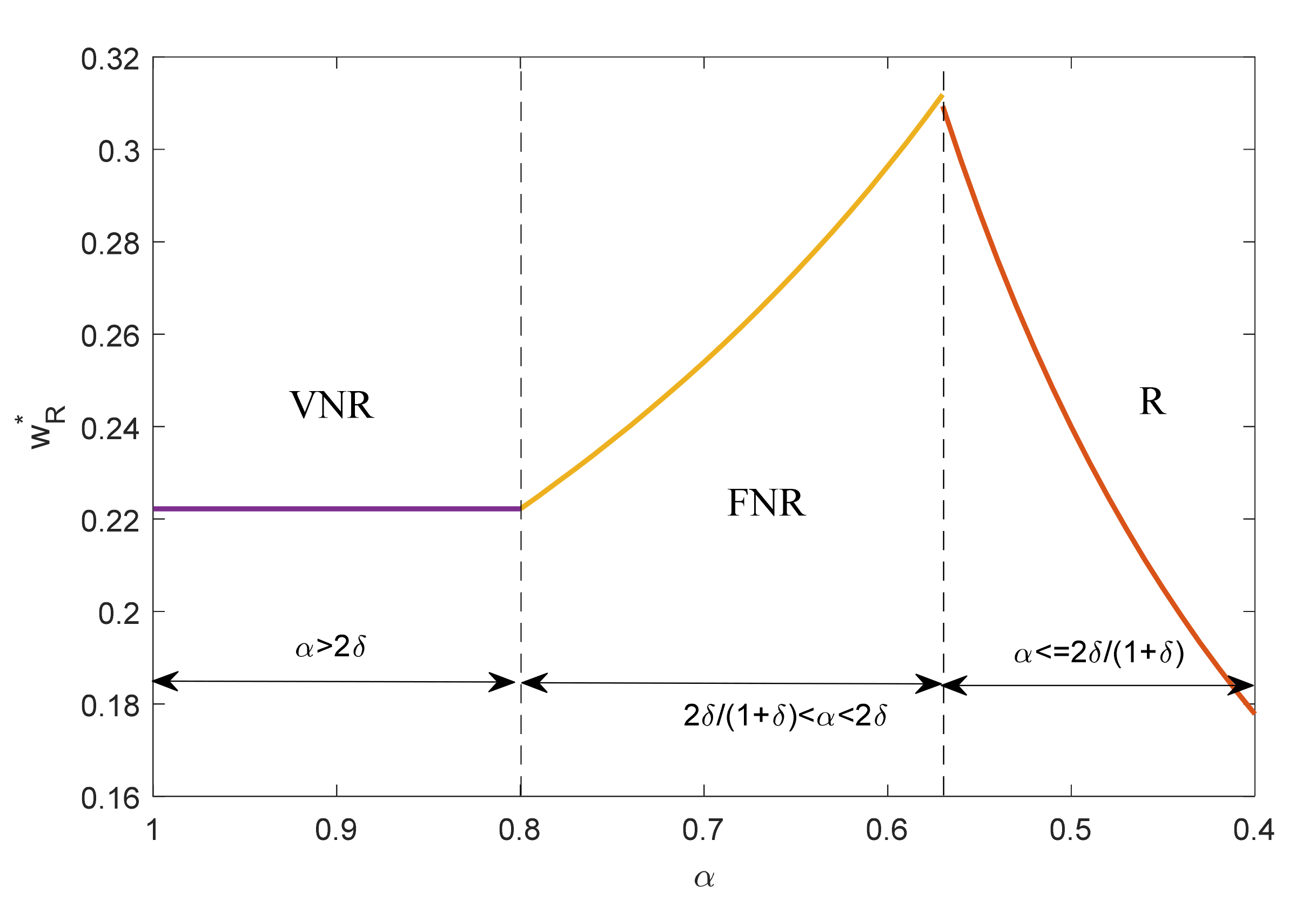
When α / δ 2 , w R * = w NR * ; when 2 / 1 + δ < α / δ < 2 , w R * > w NR * and w R * / α < 0 ; when α ˜ / δ < α / δ < 2 / 1 + δ , w R * > w NR * and w R * / α > 0 ; and when 1 < α / δ < α ˜ / δ , w R * < w NR * and w R * / α > 0 , where
α ˜ = 1 + δ 3 δ 1 + δ 2 3 δ 2 16 δ 2 δ / 4  
Figure 4 shows the change process of the new products’ wholesale prices with respect to the cost-to-value ratios of the remanufactured products, which is described in Proposition 3. When α / δ 2 , the retailer does not engage in remanufacturing, thus only new products are available in the market and the wholesale price will not change. When 2 / 1 + δ < α / δ < 2 , the OEM will improve the new products’ qualities to deter the retailer from taking part in remanufacturing; thus, the new products’ qualities increase with the decrease in the cost-to-value ratio, and the OEM also increases the wholesale prices with the increase in the qualities of the new products. When 1 < α / δ < 2 / 1 + δ , the retailer enters the remanufacturing market, and the old and new products compete in the market. With the cost-to-value ratio decreasing, the competition intensifies and prices decrease. Lower product prices lead to decreased product qualities, and the wholesale prices of new products also decrease with the decrease in product qualities. When the cost-to-value ratio decreases to a certain threshold, the wholesale prices of new products will be lower than when the retailer has not entered the remanufacturing industry. That is because competition causes the new products’ prices to decrease lower than the prices when the new products are monopolized, and the OEM will further reduce the products’ wholesale prices to increase the order quantities of new products.
Proposition 4.
Q N - R * = Q N - NR * always holds.
Proposition 4 indicates that the new products’ sales volumes remain constant whether the retailer engages in the remanufacturing operation or not. This is an interesting conclusion because it illustrates that the retailer’s participation in the remanufacturing business does not affect the sales of new products. Therefore, in some sense, remanufactured products cannot replace new products, but only increase the whole sales of remanufactured and new products. This is because the emergence of remanufactured products enables the OEM to maintain a relatively fixed price performance by improving product quality, which could stabilize the sales.
Proposition 5.
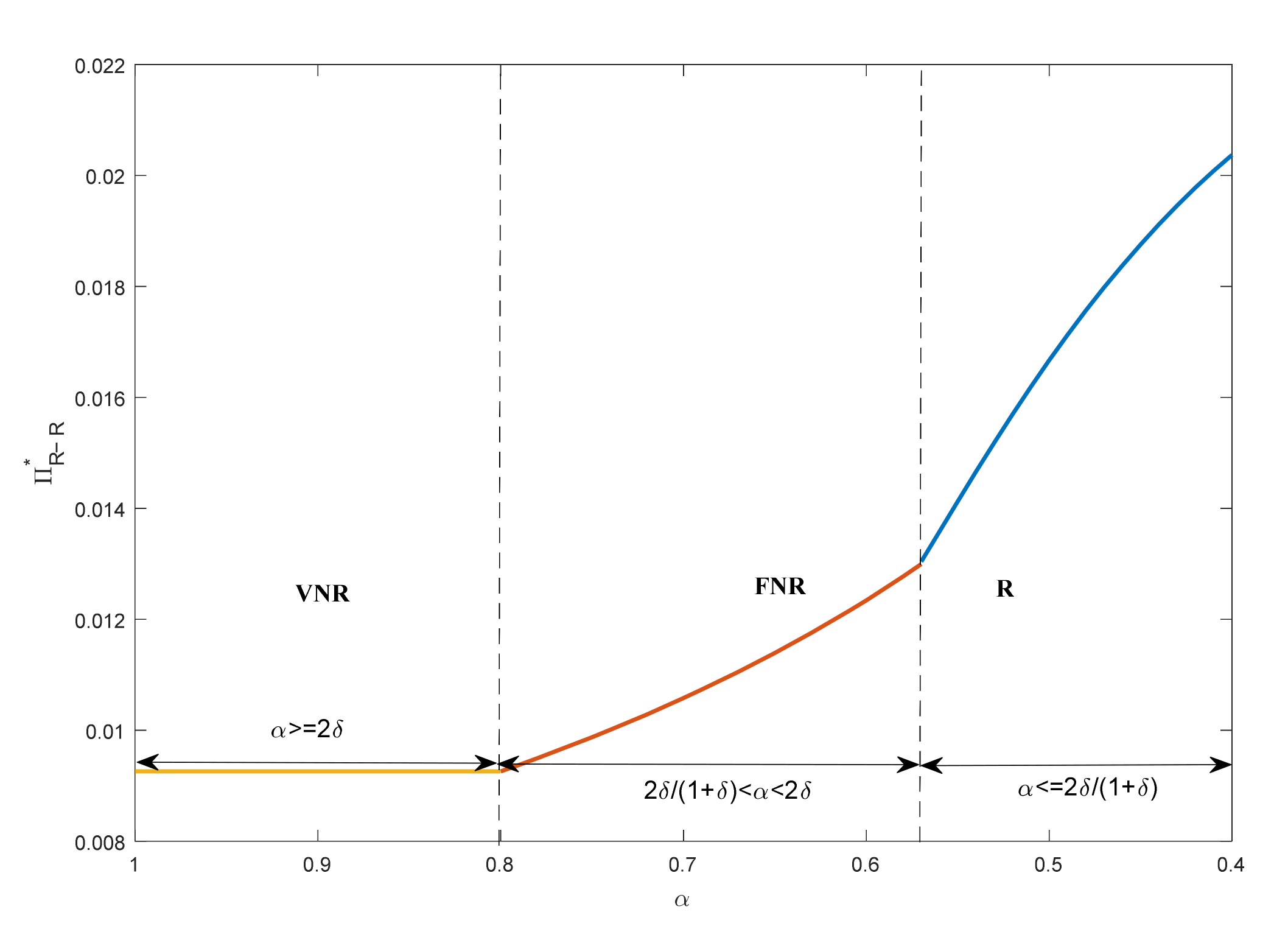
(1) Π R - R * > Π R - NR * always holds. (2) When α / δ 2 , Π OEM - R * = Π OEM - NR * ; when 1 < α / δ < 2 , Π OEM - R * < Π OEM - NR * . (3) When α / δ 2 , Π C - R * = Π C - NR * ; when 2 / 1 + δ < α / δ < 2 , Π C - R * > Π C - NR * and Π C - R * is concave and the maximum can be achieved at α = max 8 δ / 5 , 2 δ / 1 + δ ; when 1 < α / δ < 2 / 1 + δ , if 3 δ 2 1 2 δ + 1 3 δ 6 δ 2 δ 3 α 2 + 3 δ α 3 > δ 3 6 δ 6 δ 2 α , Π C - R * > Π C - NR * holds, otherwise, Π C - R * Π C - NR * .
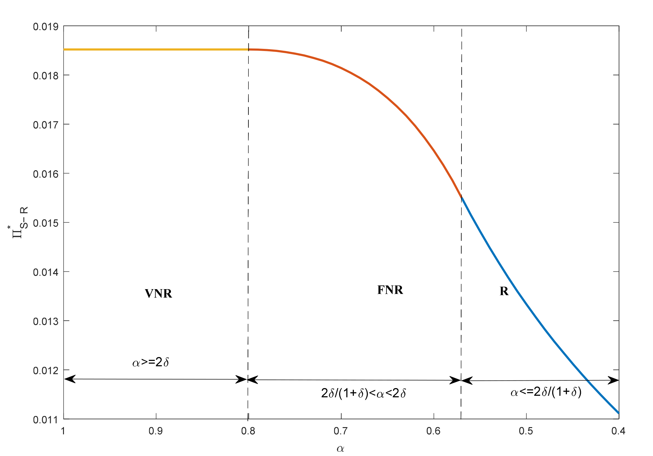
Proposition 5 (1) demonstrates that engaging in remanufacturing always brings the retailer more profit. Remanufacturing can bring new business profits to the retailer, and the profits gradually increase with the cost advantage of the remanufactured products, as illustrated in Figure 5.
Proposition 5 (2) suggests that when the retailer voluntarily gives up the remanufacturing business, it will not influence the OEM’s profit. When the cost-to-value ratio of remanufactured products decreases to a certain extent, the profitability is attractive and the retailer has the motivation to enter the remanufacturing industry. In this situation, the OEM prevents the retailer from entering the remanufacturing market by improving the qualities of new products. However, impeding the retailer from engaging in remanufacturing by improving product quality will also increase the production costs of new products, increase the wholesale price, and decrease the margin profit. When the retailer enters the remanufacturing market, the profit of the OEM will further decrease with the enhancement of remanufactured products’ cost advantages. The reason is that the competition between old and new products leads to lower prices, which will further reduce the profit of new products. Figure 6 describes the change process of OEM’s profit with the cost-to-value ratios of remanufactured products.
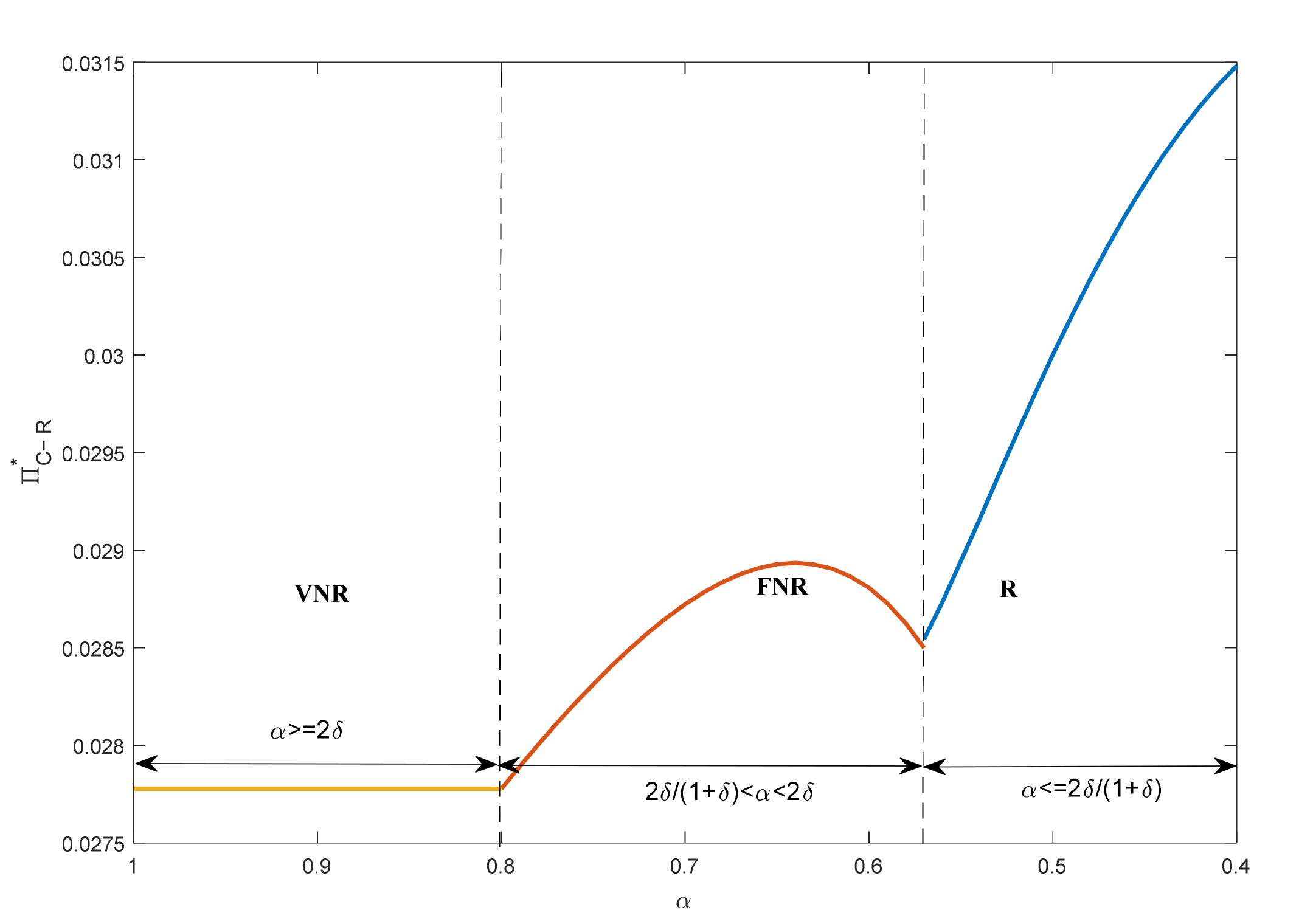
Proposition 5 (3) suggests that, from the perspective of the whole supply chain, when the retailer voluntarily gives up participating in the remanufacturing industry, the supply chain’s profit stays the same. When the cost-to-value ratio of remanufactured products decreases to a certain level, the retailer has the motivation but cannot engage in the remanufacturing operation due to the OEM’s deterrence, and thus the supply chain’s profit first increases and then decreases with the decrease in cost-to-value ratios of the remanufactured products. This is because, in this range, OEMs will improve new products’ qualities to prevent the retailer from engaging in the remanufacturing industry, which will also increase the costs of new products. At the same time, the cost advantage of products increases with the improvement of the new products’ qualities, which brings the retailer more profits. In terms of the whole supply chain, when the qualities of new products reach a certain level, the OEM’s increased cost outweighs the retailer’s increased benefit. Therefore, the profit of the supply chain first increases and then decreases. When the cost advantages of the remanufactured products further increase, the retailer enters the remanufacturing market, and the supply chain’s profit increases with the cost advantages of the remanufactured products. The average product cost in the market will decrease with the reduction of the remanufactured products’ costs, and the profit of the whole supply chain will increase. The whole process is shown in Figure 7.

4.2. Customer Surplus and Social Welfare

In this subsection, we compare customer surplus and social welfare between model NR and model R. Following Örsdemir et al. (2014) [11], we denote customer surplus as
CS = 1 Q N 1 s v p N d v + 1 Q N Q R 1 Q N s δ v p R d v
where the first term is the summation of all surplus for customers buying the new products, while the second term is the summation of all surplus for the customers buying the remanufactured products. In addition, we denote social welfare as
SS = CS + Π OEM + Π R
After substituting equilibrium results obtained previously into (10) and (11), we present the following proposition:
Proposition 6.
(1) In model NR, the customer surplus and social welfare are CS NR = 1 / 216 β and SS NR = 7 / 216 β . (2) In model R, if α / δ 2 , the customer surplus and social welfare are CS R = 1 / 216 β and SS R = 7 / 216 β ; if 2 / 2 δ < α / δ < 2 , the customer surplus and social welfare are CS R = δ / 108 α β and SS R = δ 11 α 8 δ / 108 α 2 β ; and if α / δ < 2 / 2 δ , the customer surplus and social welfare are as follows:
CS R = 1 δ δ 1 α 2 + 4 δ 3 δ α α 2 δ δ α α / 216 δ 1 α 3 β  
SS R = δ 1 δ 5 4 δ 1 α 2 + 1 δ 4 2 α 3 2 α δ 2 + 3 α 2 + 2 1 11 α + 7 α 2 δ 216 δ 1 α 3 β
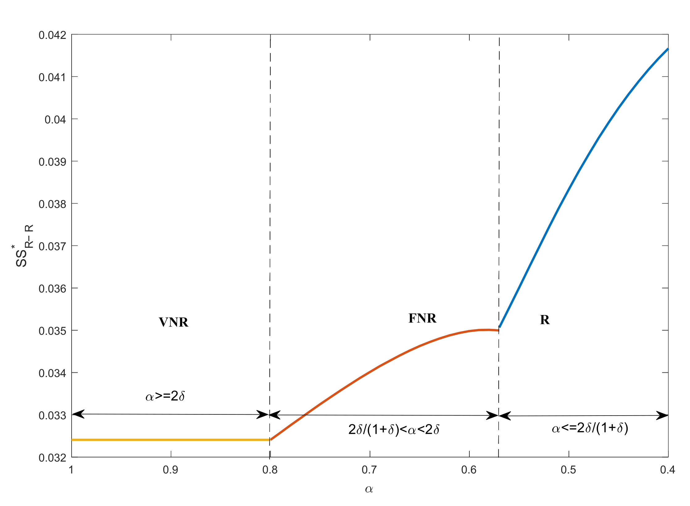
Figure 8 and Figure 9 display the change process of consumer surplus and social welfare in model R as described in Proposition 6. From Figure 8 we can see that consumer surplus increases with the remanufactured products’ cost-to-value ratio in region FNR. The reason for this is that the OEM improves the qualities of new products to deter the retailer from entering the remanufacturing market in region FNR, which improves the price performances of new products and the consumer surplus. With the enhanced remanufacturing cost advantages of the remanufactured products in region R, the retailer enters the remanufacturing industry, and the new and old products compete in the market. At this time, the prices of new and old products decrease, although the products’ qualities also decrease, the overall price performance increases, and the consumer surplus is further improved. Figure 9 shows the change process of social welfare. With the cost-to-value ratio of the remanufactured products decreasing in region FNR, the qualities of new products increase, and the prices of products increase. However, when a product’s quality increases to a certain level, the cost becomes too large. So, the social welfare first increases and then decreases in region FNR. As the cost advantage of the remanufactured products is further enhanced in region R, the retailer enters the remanufacturing market, the social welfare increases gradually with the enhanced remanufacturing cost advantage, and high price is brought by the competition between the new and remanufactured products.

4.3. Environmental Impact

In this subsection, we discuss how the action of retailers entering remanufacturing operations affects the environment. Following Atasu and Souza (2013) [12] and Örsdemir et al. (2014) [11], we consider the environmental impacts of the manufacturing stage, use stage, and EOL stage, denoted as e N M , e N U , e N E , e R M , e R U and e R E , where subscripts M, U, and E stand for production stage, use stage, and EOL stage, respectively, and superscripts N and R stand for new product and remanufactured product, respectively. Empirical evidence (e.g., Hauser and Lund, 2008) [9] shows that since some parts can be reused in the remanufacturing process, less raw material and energy are consumed to produce a remanufactured product than to produce a new product. Thus, we assume e N M > e R M . Based on these assumptions, the total environmental impacts in model NR and model R are as follows:
E NR = e N M + e N U + e N E 6
E R = e N M + e N U + e N E 6 ,   α δ 2 2 δ e N M + e N U 6 + α δ e N E 6 δ 1 α + 2 δ δ α α e R M + e R U + e R E 6 δ 1 α ,   α δ < 2 2 δ
According to (12) and (13), we offer the following proposition, which illustrates the environmental effect of the retailer when entering remanufacturing operations:
Proposition 7.
When a retailer enters remanufacturing operations, if and only if e N E > e R M + e R U + e R E and α / δ < 2 / 2 δ , it is beneficial for the environment.
Proposition 7 demonstrates that the action of the retailer entering the remanufacturing operation is not always good for the environment. Only when the environmental impacts of the new products in the EOL stage are larger than the total environmental impacts of the remanufactured products over their whole life cycle, along with the retailer’s cost advantage of remanufacturing, is the retailer’s action of entering the remanufacturing market good for the environment. For in this condition, the environmental impact of producing both new and old products is less than the impact of only producing new products.

5. Conclusions and Managerial Implications

We use a game-theoretical model to study how retailer-oriented remanufacturing affects OEM’s quality choice of new products, taking the NR model (the case without remanufacturing) as the benchmark. We also build a model in which the retailer develops the remanufacturing operation (Model R). We obtain some meaningful conclusions by comparing the equilibrium outcome in the two models.
We find that the retailer’s action of developing remanufacturing business always hurts the interests of the OEM due to the cannibalization. So, the OEM adjusts the products’ qualities as a strategy to deter the retailer from entering the remanufacturing market. However, this strategy is not always effective; it maintains the sales of new products but brings a higher cost which in turn hurts the OEM’s profits. We also find the key factor of the retailer’s motivation for remanufacturing and the effectiveness of the OEM’s strategy is the remanufactured products’ cost-to-value ratio, which could reflect the remanufactured products’ profitability. When the cost-to-value ratio is low, implying the remanufacturing is profitable, the retailer has an incentive to take part in the remanufacturing operation, and the OEM starts to use the strategy of raising the qualities and wholesale prices of new products to deter the retailer. If the cost-to-value ratio is not sufficiently low, the OEM’s strategy is effective, and the retailer gives up entering the remanufacturing operation after weighing the revenues from the two channels (the new and the remanufactured products). However, when the cost-to-value ratio is sufficiently low, the remanufacturing operation’s profitability increases, the retailer enters the remanufacturing market, and the OEM’s strategy fails. This leads to a further increase in the retailer’s profit and a further decrease in the OEM’s profit. Regarding the whole supply chain’s benefit, consumer surplus, and social welfare, we find that the retailer’s successful entry into the remanufacturing market and even just the threat of the retailer’s entry improves the whole supply chain’s profit, consumer surplus, and social welfare. This suggests that the retailer’s action of developing the remanufacturing operation always benefits the supply chain, consumer surplus, and social welfare.
Furthermore, this paper discusses the environmental impact of the retailer entering the remanufacturing market. According to the results, it is clear now that the retailer’s action of taking part in the remanufacturing industry is not always good for the environment. Only when the environmental impacts of the new products in the EOL stage are larger than the total environmental impacts of the remanufactured products over their whole life cycle is the retailer’s action of entering the remanufacturing market good for the environment.
The results of this study have important implications for academia, industry, and policymakers. From an academic perspective, this study broadens our understanding of remanufacturing, especially the impact of remanufacturing on product design for upstream manufacturers when the retailers implement remanufacturing. For managers, the retailers’ remanufacturing operation will increase its profits at the expense of upstream manufacturers’ profit loss. Manufacturers relying only on wholesale prices and product quality design can hardly make up for the loss caused by retailers’ development of remanufacturing operations. Therefore, designing a more effective transfer pricing mechanism, for example charging two-part tariffs or licensing fees to retailers, may be a more effective strategy. For policymakers, the results of this study suggest that encouraging retailers to develop remanufacturing is profitable for the entire supply chain and can increase consumer surplus and total social welfare. Determining how to protect the interests of upstream manufacturers and even how to share the profits brought by retailers’ development of remanufacturing are the key problems that policymakers should solve. Providing manufacturers with tax subsidies or patent protection may achieve a win–win situation.
In our current model, we only consider the single-period model. In future research, we will consider the multiperiod model, which may be more in line with reality. At the same time, our model does not take into account patent licensing fees. In the future, we will consider that retailers need to pay patent licensing fees to manufacturers to develop remanufacturing operations.

Author Contributions

Conceptualization and methodology, Z.Z.; formal analysis and writing—original draft preparation, Q.Z.; writing—review and editing, C.W. All authors have read and agreed to the published version of the manuscript.

Funding

This research was funded by the Humanities and Social Science Fund of the Ministry of Education of China, grant number 21YJC630186; the Natural Science Foundation of Guangdong Province, grant number 2022A1515012034; the Philosophy and Social Science Planning Project of Guangdong Province, grant number GD20CGL19; and the Startup Fund from Shantou University, grant number STF19024.

Conflicts of Interest

The authors declare no conflict of interest.

Appendix A

Proof of Table 2.
In model NR, the retailer’s decision problem can be expressed as
Π R - NR = max Q N s 1 Q N w Q N
Because 2 Π R - NR / Q N 2 = 2 s < 0 , the retailer’s decision problem is concave with respect to Q N . By taking the first-order condition, the retailer’s optimal response function can be obtained as follows:
Q N = s w 2 s
Substituting (A1) into the OEM’s decision problem, we have
Π OEM - NR = max s , w w β s 2 s w 2 s ,
Because 2 Π OEM - NR / w 2 = 1 s < 0 , the OEM’s decision problem is concave with respect to w , and the optimal wholesale price is
w N = s + β s 2 2 .
Then, by substituting (A2) into the OEM’s decision problem, we have
Π OEM - NR = max s s 1 β s 2 8 .
Because 2 Π OEM - NR / s 2 = β 2 3 β s 4 < 0 , the OEM’s decision problem is concave with respect to s , and the optimal quality level is
s N = 1 3 β .
From Equations (A1)–(A3), we have the equilibrium decision as follows:
s NR * = 1 3 β
w NR * = 2 9 β
Q N - NR * = 1 6
p N - NR * = 5 18 β
By substituting the equilibrium decisions into the OEM’s and retailer’s functions, equilibrium profits can be obtained as follows:
Π OEM - NR * = 1 54 β ,
Π R - NR * = 1 108 β .
 □
Proof of Table 3.
In model R, the retailer’s decision problem can be expressed as
Π R - R = max Q N , Q R s 1 Q N δ Q R w Q N + s δ 1 Q N Q R α β s 2 Q R
The second-order derivatives of Π R - R with Q N and Q R are as follows:
2 Π R - R Q N 2 = 2 s ,
2 Π R - R Q R 2 = 2 s δ ,
2 Π R - R Q N Q R = 2 Π R - R Q R Q N = 2 s δ .
The Hessian matrix according to Π R - R is as follows:
H = 2 Π R - R Q N 2 2 Π R - R Q N Q R 2 Π R - R Q R Q N 2 Π R - R Q R 2 = 2 s 2 s δ 2 s δ 2 s δ .
Because
H 1 = 2 s 0 ,
H 2 = 2 s 2 s δ 2 s δ 2 s δ = 4 δ 1 δ s 2 0 .
The profit function of the retailer is concave with Q N and Q R .
According to the following first-order condition:
Π R - R Q N = s 1 2 Q N 2 δ Q R w = 0 ,
Π R - R Q R = s δ 1 2 Q N 2 Q R α β s 2 = 0 ,
we obtain
Q N = s 1 δ + α β s w 2 s 1 δ Q R = δ w α β s 2 2 δ s 1 δ .
Substituting (A3) into the OEM’s decision problem, we have
Π OEM - R = max s , w w β s 2 s 1 δ + α β s w 2 s 1 δ
Because 2 Π OEM - NR / w 2 = 1 s 1 δ < 0 , the OEM’s decision problem is concave with respect to w , and the optimal wholesale price is
w R = s 1 δ + 1 + α β s 2 2
Substituting (A6) into the OEM’s decision problem, we have
Π OEM - R = max s s 1 δ 1 α β s 2 8 1 δ
Because 2 Π OEM - R / s 2 = 1 α β 2 1 δ 3 1 α β s 4 1 δ < 0 , the OEM’s decision problem is concave with respect to w , and the optimal wholesale price is
s = 1 δ 3 1 α β
From the Equations (A4), (A6) and (A8), we have the equilibrium decision as follows:
s R * = 1 δ 3 1 α β ,
w R * = 2 α 1 δ 2 9 1 α 2 β ,
Q N - R * = 1 6 ,
Q R - R * = 2 δ δ α α 6 δ 1 α ,
p N - R * = 5 2 δ 4 δ α 1 δ 18 1 α 2 β ,
p R - R * = 3 δ + 1 4 δ α 1 δ 18 1 α 2 β .
By substituting the equilibrium decisions into the OEM’s and retailer’s functions, equilibrium profits can be obtained as follows:
Π OEM - R * = 1 δ 2 54 β 1 α ,
Π R - R * = 1 + 2 δ 2 + δ α 1 δ 108 1 α 2 β + 1 δ 2 δ δ α α 3 δ 1 + 2 δ α 108 δ 1 α 3 β .
Then, we discuss under which condition the retailer will voluntarily give up the remanufacturing operation or is forced to abandon the remanufacturing operation. First, we discuss the condition of the retailer forced to abandon the remanufacturing operation. Assume the OEM is making the decision as in model NR; i.e., s = 1 3 β and w = 2 9 β . Substituting s = 1 3 β and w = 2 9 β into Q R = δ w α β s 2 2 δ s 1 δ , we have Q R = 2 δ α 6 δ 1 δ . Therefore, when 2 α δ , Q R * = 0 . Thus, when 2 α δ , even if the OEM does not adjust the wholesale price and the quality level of the new product, the retailer has no incentive to develop the remanufacturing operation. In this scenario, the OEM’s and the retailer’s decisions will be the same as in model NR. Next, we discuss the condition of the retailer being forced to abandon the remanufacturing operation. From the remanufacturing quantity Q R = δ w α β s 2 2 δ s 1 δ , we will find that when δ w = α β s 2 , the optimal remanufacturing quantity will be Q R - R * = 0 . Substituting δ w = α β s 2 into the OEM’s decision problem, we have
Π OEM - R = max s , w w β s 2 s 1 δ + α β s w 2 s 1 δ s . t .   δ w = α β s 2
We have the equilibrium decision as follows:
s R * = 2 δ 3 α β ,
w R * = 4 δ 9 α β ,
Q N - R * = 1 6 ,
Q R - R * = 0
p N - R * = 5 δ 9 α β .
By substituting the equilibrium decisions into the OEM’s and retailer’s functions, equilibrium profits can be obtained as follows:
Π OEM - R * = 4 δ α δ 54 α 2 β ,
Π R - R * = δ 54 α β .
 □
Proof of Proposition 1
. The results of Proposition 1 are easy to obtain from Table 3, so we omit the proof process.  □
Proof of Proposition 2.
The results of Proposition 2 are easy to obtain from Table 2 and Table 3, so we omit the proof process.  □
Proof of Proposition 3.
The results of Proposition 3 are easy to obtain from Table 2 and Table 3, so we omit the proof process.  □
Proof of Proposition 4.
The results of Proposition 4 are easy to obtain from Table 2 and Table 3, so we omit the proof process.  □
Proof of Proposition 5.
The results of Proposition 5 are easy to obtain from Table 2 and Table 3, so we omit the proof process.  □
Proof of Proposition 6.
The results of Proposition 6 are easy to obtain from Table 2 and Table 3, so we omit the proof process.  □

References

  1. Huang, Z.; Shao, W.; Meng, L.; Zhang, G.; Qiang, Q. Pricing Decision for a Closed-Loop Supply Chain with Technology Licensing under Collection and Remanufacturing Cost Disruptions. Sustainability 2022, 14, 3354. [Google Scholar] [CrossRef]
  2. Zhang, X.; Cao, J.; Zhao, Y.; Lu, J. Fairness Concern in Remanufacturing Supply Chain—A Comparative Analysis of Channel Members’ Fairness Preferences. Sustainability 2022, 14, 3813. [Google Scholar] [CrossRef]
  3. Atasu, A.; Guide, V.D.R.; Van Wassenhove, L.N. So What If Remanufacturing Cannibalizes My New Product Sales? Calif. Manag. Rev. 2010, 52, 1–21. [Google Scholar] [CrossRef] [Green Version]
  4. Giutini, R.; Gaudette, K. Remanufacturing: The next great opportunity for boosting US productivity. Bus. Horiz. 2003, 46, 41–48. [Google Scholar] [CrossRef]
  5. Gao, J.; Han, H.; Wang, H. Pricing and effort decisions in a closed-loop supply chain under different channel power structures. J. Clean. Prod. 2016, 112, 2043–2057. [Google Scholar] [CrossRef]
  6. Guide, V.D.R.; Harrison, T.P.; Van Wassenhove, L.N. The challenge of closed-loop supply chains. INFORMS J. Appl. Anal. 2003, 33, 3–6. [Google Scholar] [CrossRef]
  7. Ferguson, M.E.; Souza, G.C. Closed-Loop Supply Chains—New Developments to Improve the Sustainability of Business Practices; Taylor & Francis Group: Oxford, UK, 2010. [Google Scholar]
  8. Ovchinnikov, A.; Blass, V.; Raz, G. Economic and Environmental Assessment of Remanufacturing Strategies for Product + Service Firms. Prod. Oper. Manag. 2014, 23, 744–761. [Google Scholar] [CrossRef]
  9. Hauser, W.M.; Lund, R.T. Remanufacturing: Operating Practices and Strategies; Boston University: Boston, MA, USA, 2008. [Google Scholar]
  10. Yi, P.; Huang, M.; Guo, L.; Shi, T. Dual recycling channel decision in retailer oriented closed-loop supply chain for construction machinery remanufacturing. J. Clean. Prod. 2016, 137, 1393–1405. [Google Scholar] [CrossRef]
  11. Örsdemir, A.; Kemahlıoğlu-Ziya, E.; Parlaktürk, A.D. Competitive quality choice and remanufacturing. Prod. Oper. Manag. 2014, 23, 48–64. [Google Scholar] [CrossRef]
  12. Atasu, A.; Souza, G.C. How does product recovery affect quality choice? Prod. Oper. Manag. 2013, 22, 991–1010. [Google Scholar] [CrossRef]
  13. Qian, Z.; Chai, J.; Li, H.; Yan, W.; Chen, H. Implications of product upgrading confronting supplier remanufacturing. Int. J. Prod. Res. 2020, 58, 5870–5892. [Google Scholar] [CrossRef]
  14. Zou, Z.; Wang, F.; Lai, X.; Hong, J. How Does Licensing Remanufacturing Affect the Supply Chain Considering Customer Environmental Awareness? Sustainability 2019, 11, 1898. [Google Scholar] [CrossRef] [Green Version]
  15. Atasu, A.; Sarvary, M.; Van Wassenhove, L.N. Remanufacturing as a Marketing Strategy. Manag. Sci. 2008, 54, 1731–1746. [Google Scholar] [CrossRef] [Green Version]
  16. Chen, J.; Chang, C. The co-opetitive strategy of a closed-loop supply chain with remanufacturing. Transp. Res. Part E Logist. Transp. Rev. 2012, 48, 387–400. [Google Scholar] [CrossRef]
  17. Zou, Z.; Wang, J.; Deng, G.; Chen, H. Third-party remanufacturing mode selection: Outsourcing or authorization? Transp. Res. Part E Logist. Transp. Rev. 2016, 87, 1–19. [Google Scholar] [CrossRef]
  18. Savaskan, R.C.; Bhattacharya, S.; Van Wassenhove, L.N. Closed-loop supply chain models with product remanufacturing. Manag. Sci. 2004, 50, 239–252. [Google Scholar] [CrossRef] [Green Version]
  19. Abbey, J.D.; Meloy, M.G.; Guide, V.D.R.; Atalay, S. Remanufactured products in closed-loop supply chains for consumer goods. Prod. Oper. Manag. 2015, 24, 488–503. [Google Scholar] [CrossRef]
  20. Jena, S.K.; Sarmah, S.P. Price and service co-opetiton under uncertain demand and condition of used items in a remanufacturing system. Int. J. Prod. Econ. 2016, 173, 1–21. [Google Scholar] [CrossRef]
  21. Chen, X.; Cao, J.; Kumar, S. Government regulation and enterprise decision in China remanufacturing industry: Evidence from evolutionary game theory. Energy Ecol. Environ. 2021, 6, 148–159. [Google Scholar] [CrossRef]
  22. Mitra, S.; Webster, S. Competition in remanufacturing and the effects of government subsidies. Int. J. Prod. Econ. 2008, 111, 287–298. [Google Scholar] [CrossRef]
  23. He, P.; He, Y.; Xu, H. Channel structure and pricing in a dual-channel closed-loop supply chain with government subsidy. Int. J. Prod. Econ. 2019, 213, 108–123. [Google Scholar] [CrossRef]
  24. Xiong, Y.; Li, G.; Zhou, Y.; Fernandes, K.; Harrison, R.; Xiong, Z. Dynamic pricing models for used products in remanufacturing with lost-sales and uncertain quality. Int. J. Prod. Econ. 2014, 147, 678–688. [Google Scholar] [CrossRef]
  25. Han, X.H.; Wu, H.Y.; Yang, Q.X.; Shang, J. Collection channel and production decisions in a closed-loop supply chain with remanufacturing cost disruption. Int. J. Prod. Res. 2017, 55, 1147–1167. [Google Scholar] [CrossRef]
  26. Sun, H.; Chen, W.; Liu, B.; Chen, X. Economic lot scheduling problem in a remanufacturing system with returns at different quality grades. J. Clean. Prod. 2018, 170, 559–569. [Google Scholar] [CrossRef]
  27. Baghdadi, E.; Shafiee, M.; Alkali, B. Upgrading Strategy, Warranty Policy and Pricing Decisions for Remanufactured Products Sold with Two-Dimensional Warranty. Sustainability 2022, 14, 7232. [Google Scholar] [CrossRef]
  28. Li, X.; Cui, X.; Li, Y.; Xu, D.; Xu, F. Optimisation of reverse supply chain with used-product collection effort under collector’s fairness concerns. Int. J. Prod. Res. 2019, 59, 652–663. [Google Scholar] [CrossRef]
  29. Matsumoto, M. Development of a simulation model for reuse businesses and case studies in Japan. J. Clean. Prod. 2010, 18, 1284–1299. [Google Scholar] [CrossRef]
  30. Subramanian, R.; Subramanyam, R. Key factors in the market for remanufactured products. Manuf. Serv. Oper. Manag. 2012, 14, 315–326. [Google Scholar] [CrossRef] [Green Version]
  31. Yan, W.; Xiong, Y.; Xiong, Z.; Guo, N. Bricks vs. clicks: Which is better for marketing remanufactured products? Eur. J. Oper. Res. 2015, 242, 434–444. [Google Scholar] [CrossRef]
  32. Yenipazarli, A. Managing new and remanufactured products to mitigate environmental damage under emissions regulation. Eur. J. Oper. Res. 2016, 249, 117–130. [Google Scholar] [CrossRef]
  33. Neto, J.Q.; Bloemhof, J. An Analysis of the Eco-Efficiency of Remanufactured Personal Computers and Mobile Phones. Prod. Oper. Manag. 2012, 21, 101–114. [Google Scholar] [CrossRef]
  34. Gu, W.; Chhajed, D.; Petruzzi, N.C.; Yalabik, B. Quality design and environmental implications of green consumerism in remanufacturing. Int. J. Prod. Econ. 2015, 162, 55–69. [Google Scholar] [CrossRef] [Green Version]
  35. Chaowanapong, J.; Jongwanich, J.; Ijomah, W. Factors influencing a firm’s decision to conduct remanufacturing: Evidence from the Thai automotive parts industry. Prod. Plan. Control. 2017, 28, 1139–1151. [Google Scholar] [CrossRef]
  36. Kerr, W.; Ryan, C. Eco-efficiency gains from remanufacturing: A case study of photocopier remanufacturing at Fuji Xerox Australia. J. Clean. Prod. 2001, 9, 75–81. [Google Scholar] [CrossRef]
  37. Hellofs, L.L.; Jacobson, R. Market Share and Customers’ Perceptions of Quality: When Can Firms Grow Their Way to Higher versus Lower Quality? J. Mark. 1999, 63, 16–25. [Google Scholar]
  38. Gupta, R.; Biswas, I.; Kumar, S. Pricing decisions for three-echelon supply chain with advertising and quality effort-dependent fuzzy demand. Int. J. Prod. Res. 2019, 57, 2715–2731. [Google Scholar] [CrossRef]
  39. Xie, G.; Yue, W.; Wang, S.; Lai, K.K. Quality investment and price decision in a risk-averse supply chain. Eur. J. Oper. Res. 2011, 214, 403–410. [Google Scholar] [CrossRef]
  40. Ma, P.; Wang, H.; Shang, J. Contract design for two-stage supply chain coordination: Integrating manufacturer-quality and retailer-marketing efforts. Int. J. Prod. Econ. 2013, 146, 745–755. [Google Scholar] [CrossRef]
  41. Hsieh, C.C.; Liu, Y.T. Quality investment and inspection policy in a supplier–manufacturer supply chain. Eur. J. Oper. Res. 2010, 202, 717–729. [Google Scholar] [CrossRef]
  42. Veldman, J.; Gaalman, G. A model of strategic product quality and process improvement incentives. Int. J. Prod. Econ. 2014, 149, 202–210. [Google Scholar] [CrossRef]
  43. Liu, B.; Ma, S.; Guan, X.; Xiao, L. Timing of sales commitment in a supply chain with manufacturer-quality and retailer-effort induced demand. Int. J. Prod. Econ. 2018, 195, 249–258. [Google Scholar] [CrossRef]
  44. Liu, G.; Zhang, J.; Tang, W. Joint dynamic pricing and investment strategy for perishable foods with price-quality dependent demand. Ann. Oper. Res. 2014, 226, 397–416. [Google Scholar] [CrossRef]
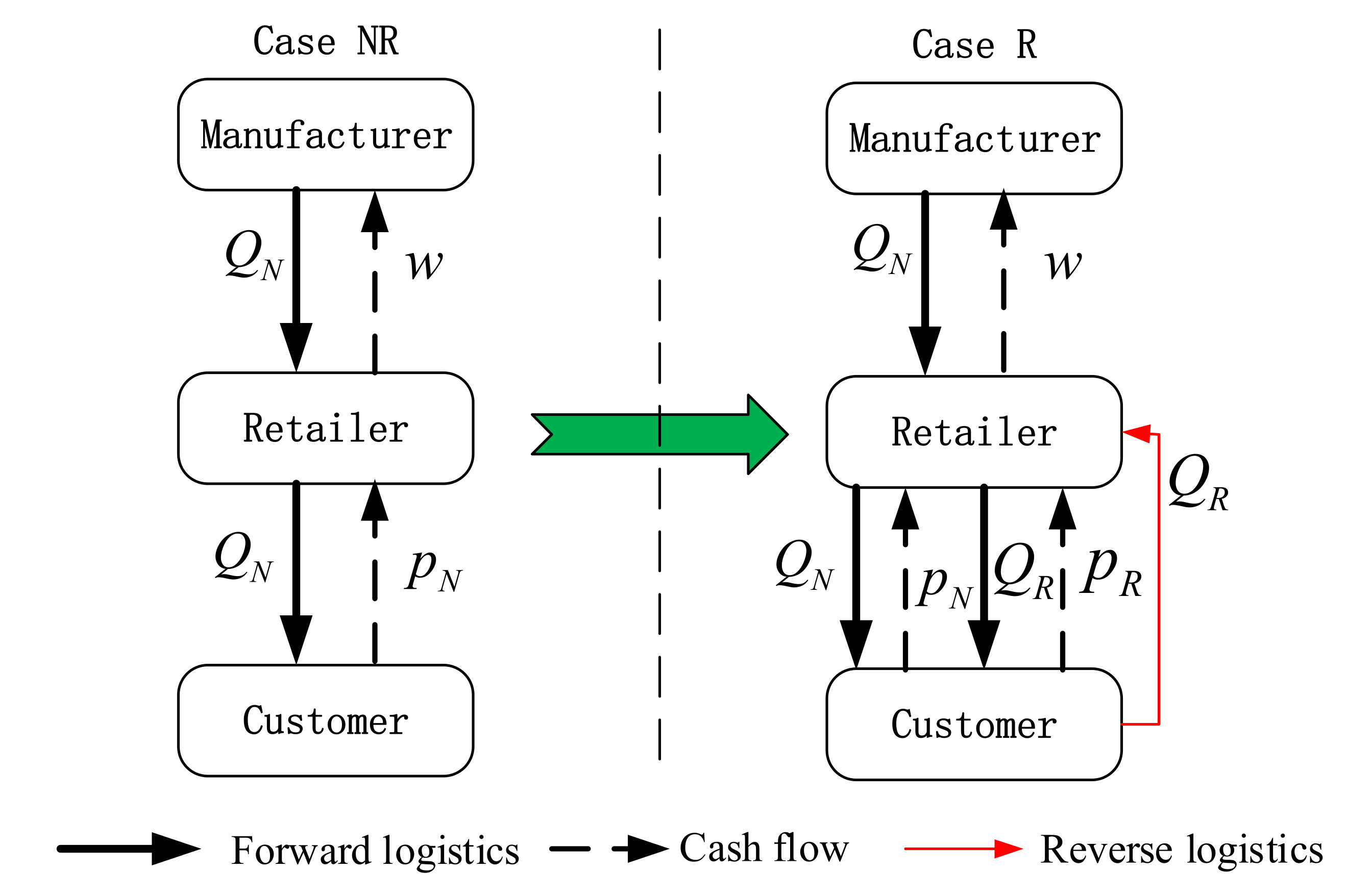
Figure 1. Supply chain structure without and with remanufacturing.
Sustainability 14 08028 g001
Figure 2. Equilibrium regions of remanufacturing strategy.
Sustainability 14 08028 g002
Figure 3. Equilibrium OEM’s new products’ qualities.
Sustainability 14 08028 g003
Figure 4. Equilibrium wholesale price of the new products.
Sustainability 14 08028 g004
Figure 5. The change in retailer’s profits.
Sustainability 14 08028 g005
Figure 6. The change in OEM’s profits.
Sustainability 14 08028 g006
Figure 7. The change in central supply-chain profits.
Sustainability 14 08028 g007
Figure 8. Consumer surplus change.
Sustainability 14 08028 g008
Figure 9. Social surplus change.
Sustainability 14 08028 g009
Table 1. Notation summary.
SymbolDefinition
v The consumers willing to pay for the new product
δ The valuation of the remanufactured products relative to the new products
s The quality level of the new products
α The ratio of unit variable cost of remanufactured product to new product
w The wholesale price of the new products
Q N The quantity of the new products
p N The price of the new products
Q R The quantity of the remanufactured products
p R The price of the remanufactured products
Table 2. The equilibrium results in model NR.
VariableEquilibrium Result
s NR * 1 3 β
w NR * 2 9 β
Q N - NR * 1 6
p N - NR * 5 18 β
Π R - NR * 1 108 β
Π OEM - NR * 1 54 β
Table 3. The equilibrium results in model R.
VariableEquilibrium Result
Range α / δ > 2 2 / 1 + δ < α / δ < 2 α / δ < 2 / 1 + δ
s R * 1 3 β 2 δ 3 α β 1 δ 3 1 α β
w R * 2 9 β 4 δ 9 α β 2 α 1 δ 2 9 1 α 2 β
Q N - R * 1 6 1 6 1 6
Q R - R * 00 2 δ δ α α 6 δ 1 α
p N - R * 5 18 β 5 δ 9 α β 5 2 δ 4 δ α 1 δ 18 1 α 2 β
p R - R * NANA 3 δ + 1 4 δ α 1 δ 18 1 α 2 β
Π R - R * 1 108 β δ 54 α β 1 + 2 δ 2 + δ α 1 δ 108 1 α 2 β + 1 δ 2 δ δ α α 3 δ 1 + 2 δ α 108 δ 1 α 3 β
Π OEM - R * 1 54 β 4 δ α δ 54 α 2 β 1 δ 2 54 β 1 α
Publisher’s Note: MDPI stays neutral with regard to jurisdictional claims in published maps and institutional affiliations.