Sustainable Circular Supplier Selection in the Power Battery Industry Using a Linguistic T-Spherical Fuzzy MAGDM Model Based on the Improved ARAS Method

Abstract

In the power battery industry, the selection of an appropriate sustainable recycling supplier (SCS) is a significant topic in circular supply chain management. Evaluating and selecting a SCS for spent power batteries is considered a complex multi-attribute group decision-making (MAGDM) problem closely related to the environment, economy, and society. The linguistic T-spherical fuzzy (Lt-SF) set (Lt-SFS) is a combination of a linguistic term set and a T-spherical fuzzy set (T-SFS), which can accurately describe vague cognition of human and uncertain environments. Therefore, this article proposes a group decision-making methodology for a SCS selection based on the improved additive ratio assessment (ARAS) in the Lt-SFS context. This paper extends the Lt-SF generalized distance measure and defines the Lt-SF similarity measure. The Lt-SF Heronian mean (Lt-SFHM) operator and its weighted form (i.e., Lt-SFWHM) were developed. Subsequently, a new Lt-SF MAGDM model was constructed by integrating the LT-SFWHM operator, generalized distance measure, and ARAS method. In it, the expert weight on the attribute was determined based on the similarity measure, using the generalized distance measure to obtain the objective attribute weight and then the combined attribute weight. Finally, a real case of SCS selection in the power battery industry is presented for demonstration. The effectiveness and practicability of this method were verified through a sensitivity analysis and a comparative study with the existing methods.

1. Introduction

The concept of industrial ecology [1,2,3] has received extensive attention due to massive waste generation, excessive consumption of natural resources, climate change, global warming, and scarcity of renewable resources. With the development of industrial ecology, the eco-industrial system (established according to the principles of natural ecology) has promoted changes in economic development and the development of the circular economy. Nakajima [4] indicated that industrial ecology can help in the transition to a more circular economy. From a systematic point of view, the goal of a circular economy is to improve the environmental/resource benefits under the premise of creating economic benefits through the circular flow of resources [5,6]. Moreover, the 6Rs (e.g., reuse, recycle, reduce, repair, redesign, and remanufacturing) have been widely recognized and understood by people [7,8].

Presently, many scholars focus on circular supply chain management in the circular economy field [9]. The circular supply chain changes the previous linear supply chain model, integrates the 6Rs of the circular economy into the supply chain, and provides a sustainable solution for modern organizations. It is insufficient for manufacturing companies in developing countries (compared with developed countries) to combine the circular supply chain with sustainable development strategies [10,11,12]. Let us use the power battery in China as an example. As the Chinese government has, for many years, been vigorously promoting the development of new energy vehicles, the total scrap volume of first-generation power batteries reached its peak in around 2021. The spent power batteries flow to the recycling company and are produced into recycled materials. For instance, 75–90% of nickel, cobalt, manganese, lithium, and other resources can be recycled through physical dismantling and smelting processes, which have relatively considerable economic benefits. These recycled materials flow back to power battery and vehicle manufacturers, forming a complete loop of “manufacturing-sales-use-recycling-manufacturing” [5,13,14]. Although the development of the power battery circular supply chain is just starting in China, its role cannot be ignored. The recycling company, as a circular supplier of the power battery manufacturer, cannot only eliminate the environmental pollution and resource waste of the spent power batteries but also save the purchasing costs of raw materials for battery manufacturers. At present, there are more than 30 large-scale and professional spent power battery recycling companies in China, such as Gremmei, Huayou Guye, Bangpu Group, Ganzhou Haopeng, etc. However, due to the concerns of power battery manufacturers about the quality of recycled materials, as well as the uncertainty of supply continuity and price fluctuation, it is challenging (but of great practical significance) for power battery manufacturers to select SCSs.

Selecting the best SCS can be regarded as a multi-criteria decision-making (MCDM) problem involving quantitative and qualitative uncertain information. For that matter, few papers focus on the evaluation and analysis of SCSs. For example, the best–worst method (BWM) and the VlseKriterijumska Optimizacija I Kompromisno Resenje (VIKOR) method were adopted by Kannan et al. to solve the problem of SCS in the polyvinyl chloride industry [15]. Liu et al. [16] developed the EDAS method based on divergence measures under the Pythagorean fuzzy set (PyFS) environment to deal with the SCS selection in the manufacturing industry. To determine the best SCS in the petrochemical industry, Mina et al. [17] applied the integration method of the fuzzy analytic hierarchy process (FAHP), the technique for order of preference by similarity to ideal solution (TOPSIS), and the fuzzy inference system. Similarly, Alavi et al. [18] applied the integration method of the fuzzy BWM and the fuzzy inference system. Nasr et al. [19] applied the fuzzy BWM and the consistency ratio algorithm to determine the optimal SCS. Haleem et al. [20] employed the fuzzy TOPSIS technique to consider the combined attribute weight (in which the objective weight was obtained by CRITIC) to determine the best SCS in the automobile manufacturing industry. Perҫin [21] applied AHP and complex proportional assessment (COPRAS) techniques to evaluate and analyze SCSs in an interval-valued intuitionistic fuzzy set (IFS) context. Bai et al. [22] constructed a group decision-making model integrating BWM-DHF (dual hesitant fuzzy)-RT (regret theory) and applied it to the circular economy and circular supplier evaluation. However, there is no more effective way to express vague and uncertain information about the SCS selection in the power battery industry.

Owing to the complexity of actual MCDM, the crisp values are no longer suitable for the alternative evaluation. Therefore, the concepts of IFS [23] and PyFS [24] were proposed on the basis of the classical fuzzy set (FS) [25]. To overcome the disadvantage that the sum of squares of the membership degree (MD) and non-membership degree (ND) in the Pythagorean fuzzy number is greater than one, the notion of the q-rung orthopair fuzzy set (q-ROFS) was proposed by Yager [26], characterized by the sum of the q-power of MD and ND being less than or equal to one. Therefore, the q-ROFS is considered a generalized structure of the classical fuzzy set, IFS and PyFS. Subsequently, the concept of the picture fuzzy set (PFS) was introduced by Cuong [27]. The abstinence degree (AD), compared with IFS, was added, so that the sum of MD, AD, and ND was no higher than one. The spherical fuzzy set (SFS), inspired by the PyFS, was defined by Ashraf et al. [28]; Mahmood et al. [29] introduced the broader idea of the T-spherical fuzzy set (T-SFS). The characteristics of T-SFS are that the sums of the q-power of MD, AD, and ND are no higher than one, which means more decision-making space, allowing decision-makers (DMs) to depict their opinions of objects more freely. As shown in Figure 1, there are connections and differences between the above different types of fuzzy sets in terms of dimensions and power numbers. The practical MCDM problem itself has uncertain information, including unquantifiable, incomplete, or unattainable information. However, it is not easy for DMs to represent the degrees of uncertainty by relying on accurate data. In particular, when assessing system performance, the DMs prefer to use linguistic evaluation [30], such as “good”, “very likely”, “low”, etc. These linguistic terms can be intuitive and easy to understand, close to a person’s cognition. However, considering that a single linguistic variable cannot completely portray the actual ideas of DMs, Chen and Liu [31] proposed that the linguistic intuitionistic fuzzy number (LIFN) forms the intuitionistic fuzzy number and linguistic variable, in which the MD and ND are represented by linguistic variables. Thus, the relevant extended concepts have been put forward successively, such as linguistic Pythagorean fuzzy number (LPyFN) [32], linguistic q-rung orthopair fuzzy number (Lq-ROFN) [33], linguistic picture fuzzy number (LPFN) [34], linguistic spherical fuzzy number (LSFN) [35], and the linguistic T-spherical fuzzy number (Lt-SFN) [36]. Obviously, the Lt-SFN is a generalized form of the above-extended concepts, and its ability to express information is better than the former. Therefore, this article employs the Lt-SFN to represent a broader range of linguistic information for the power battery SCS evaluation and analysis.

As an effective alternative ranking technology, the ARAS method was first proposed by Zavadskas and Turskis [37]. The main steps of this method involve the construction of the decision matrix, data normalization, definition of the normalized weighted matrix, calculation of optimal function and utility degree, and the final ranking of alternatives [38]. The ARAS method attempts to simplify complex decision problems and choose the optimal option by relative index (utility degree). This index can reflect the difference between the alternative and the ideal solution, and eliminate the influence of different measurement units [38]. TOPSIS [39], VIKOR [40], EDAS [41], TODIM [42] have disadvantages, such as complex calculations, pre-setting of the parameters, and ignoring the relative importance of distance, but the ARAS can be directly proportional to the attribute weight and deal with complex decision-making problems. Meanwhile, its calculation process is simple and the result is reasonable. In the past six years, many scholars have carried out extensive research on the ARAS method in different environments. For example, Nguyen et al. [43] designed a selection method of conveyor equipment based on fuzzy AHP-ARAS. The fuzzy ARAS method was employed by Rostamzadeh et al. to measure the supply chain management performance of small- and medium-sized enterprises [44]. Radović et al. [45] applied the integration of ARAS and a rough set to evaluate the merits of transportation enterprises in developing countries. The BWM-ARAS technique was designed by Liao et al. to solve the problem of the digital supply chain finance supplier selection in a hesitant linguistic environment [46]. For MAGDM problems, Liu and Cheng [47] extended the ARAS method in the probability multi-valued neutrosophic context. Mallick and Pramanik [48] further extended the ARAS method to the trapezoidal neutrosophic environment. The ARAS method was extended in the PFS environment by Jovcic et al. to settle the problem of choosing the (idea of) freight distribution [49]. Mishra et al. [50] extended the ARAS method in the IFS environment and applied it for personnel IT selection. Gül [51] proposed the Fermatean fuzzy SAW-ARAS-VIKOR-integrated method to solve the COVID-19-testing laboratory selection problem. Furthermore, Gül [52] extended the ARAS method in the SFS environment. Mishra and Rani [53] presented the q-ROF ARAS method based on entropy and discrimination measures, used to deal with the sustainable recycling partner selection. However, there are still three shortcomings in the above ARAS extension study. (1) The interrelationship between attributes is ignored in the calculation of the ARAS method. (2) When determining the utility degree, the deviation from the alternative to the ideal solution is expressed by using the proportion form of crisp value after defuzzification, while the situation involving the minimal or zero denominators is ignored, resulting in no practical meaning of the utility degree. (3) There are no studies to develop the ARAS method in the Lt-SFS environment. In conclusion, it is necessary to extend and improve the ARAS method in the Lt-SFS environment to solve the power battery SCS selection problem in this manuscript.

Based on the above arguments and motivations, the contributions of this manuscript are presented below:

• The generalized distance and similarity measures of Lt-SFNs are defined, and the objective weight of the attributes and the weight of experts on the attributes are calculated (based on them, respectively).
• This paper developed two novel aggregation operators under the Lt-SFS environment—Lt-SFHM and Lt-SFWHM.
• The ARAS method is extended and improved in the Lt-SF context, where the interrelationship between attributes is captured by the Lt-SFWHM operator, and the Lt-SF generalized distance measure represents the deviation from the alternative to the ideal solution.
• The improved ARAS-based Lt-SF MAGDM model is applied to a real SCS selection in China’s power battery industry; the practicality and validity of the proposed method were tested.

To this end, the remainder of the paper is organized as follows. Section 2 briefly reviews several related basic ideas and defines two information measures. Section 3 presents the Lt-SFHM and Lt-SFWHM operators. Section 4 builds the improved ARAS model with the combined attribute weights for the Lt-SF MAGDM problems. Section 5 employs a case of the SCS selection to demonstrate the applicability of the proposed method. At the same time, the sensitivity analysis and comparative studies are performed. Section 6 concludes the work and describes future research plans.

2. Preliminaries

2.1. LTVs, T-SFSs, Lt-SFSs

Definition 1

([30]). Let linguistic term sets S = {s₀,s₁, …, s_k−1} be composed of k elements, in which k is an odd number. Generally, k = 3, 5, 7, 9. For instance, k = 7,S = {s₀, s₁, s₂, s₃, s₄, s₅, s₆} = {very low, low, medium low, medium, medium high, high, very high}.

For any linguistic set S, the following conditions should be satisfied [30]:

(1) 

If m > n, then s_m > s_n;

(2) 

If there is a negative operator neg(s_m) = s_n, then n = k − 1 − m;

(3) 

If s_m ≥ s_n, then max(s_m,s_n) = s_m;

(4) 

If s_m ≤ s_n, then min(s_m,s_n) = s_m.

Definition 2

([29]). Suppose X is a universe set, and then the form of T-SFS is described as below:

$$\Im =\left\{\langle x,\left({\tau }_{\Im }(x),{\eta }_{\Im }(x),{\vartheta }_{\Im }(x)\right)\rangle |x\in X\right\}$$

(1)

in which${\tau }_{\Im }(x),{\eta }_{\Im }(x),{\vartheta }_{\Im }(x)$are, respectively, the MD, AD, and ND of element x ∈ ℑ in X; that is, ${\tau }_{\Im }(x),{\eta }_{\Im }(x),{\vartheta }_{\Im }(x)\in [0,1]$, and meeting $0\le {\tau }_{\Im }^q(x)+{\eta }_{\Im }^q(x)+{\vartheta }_{\Im }^q(x)\le 1$, q ≥ 1 for ∀ x ∈ X. ${\pi }_{\Im }(x)=\sqrt[q]{1-{\tau }_{\Im }^q(x)-{\eta }_{\Im }^q(x)-{\vartheta }_{\Im }^q(x)}$ is named the refusal degree (RD). For simplicity, the T-spherical fuzzy number (T-SFN) is represented as a triplet of τ, η and ϑ, and denoted as χ = (τ, η, ϑ).

Definition 3

([36]). Suppose Y is a fixed domain, then an Lt-SFS form in Y is defined as follows:

$$\Delta =\left\{\left(y,s_{\tau }(y),s_{\eta }(y),s_{\vartheta }(y)\right)|y\in Y\right\}$$

(2)

in which$s_{\tau }(y),s_{\eta }(y),s_{\vartheta }(y)\in S_{[0,k]}$, s_τ(y), s_η(y), and s_ϑ(y) are, respectively, the linguistic MD, linguistic AD, and linguistic ND. They meet ${\tau }^q+{\eta }^q+{\vartheta }^q\le k^q$ (q ≥ 1) for ∀y ∈ Y. For any Lt-SFS Δ, y ∈ Y, $\pi (y)=s_{{(k^q-({\tau }^q+{\eta }^q+{\vartheta }^q))}^{1/q}}$ is named the linguistic RD. For simplicity, the linguistic T-spherical fuzzy number (Lt-SFN) is represented as $\delta =\left(s_{\tau },s_{\eta },s_{\vartheta }\right)$.

Definition 4

([36]). Suppose δ = (s_τ, s_η, s_ϑ) is a Lt-SFN, then its score function sc(δ) and accuracy function ac(δ) can be described as below:

$$sc(\delta )=s_{{(0.5\times (k^q+{\tau }^q-{\vartheta }^q))}^{1/q}}$$

(3)

$$ac(\delta )=s_{{({\tau }^q+{\eta }^q+{\vartheta }^q)}^{1/q}}$$

(4)

Theorem 1

[36].Suppose ${\delta }_1=\left(s_{{\tau }_1},s_{{\eta }_1},s_{{\vartheta }_1}\right)$ and ${\delta }_2=\left(s_{{\tau }_2},s_{{\eta }_2},s_{{\vartheta }_2}\right)$ are two Lt-SFNs, the comparison rules between δ₁ and δ₂ are described as follows:

(1) 

If sc(δ₁) > sc(δ₂), then δ₁ is greater than δ₂, namely, δ₁ > δ₂;

(2) 

If sc(δ₁) = sc(δ₂), then (i) if ac(δ₁) > ac(δ₂), then δ₁ is greater than δ₂, namely, δ₁ > δ₂; (ii) if ac(δ₁) = ac(δ₂), thenδ₁ is equal to δ₂, namely, δ₁ = δ₂.

Definition 5

([36]). Suppose ${\delta }_1=\left(s_{{\tau }_1},s_{{\eta }_1},s_{{\vartheta }_1}\right)$ and ${\delta }_2=\left(s_{{\tau }_2},s_{{\eta }_2},s_{{\vartheta }_2}\right)$ are any two Lt-SFNs, then their basic operational rules are presented as follows:

(1)

${\delta }_1\oplus {\delta }_2=\left(s_{k{(1-(1-{({\tau }_1/k)}^q)(1-{({\tau }_2/k)}^q))}^{1/q}},s_{{\eta }_1{\eta }_2/k},s_{{\vartheta }_1{\vartheta }_2/k}\right)$;

(2)

${\delta }_1\otimes {\delta }_2=\left(s_{{\tau }_1{\tau }_2/k},s_{k{(1-(1-{({\eta }_1/k)}^q)(1-{({\eta }_2/k)}^q))}^{1/q}},s_{k{(1-(1-{({\vartheta }_1/k)}^q)(1-{({\vartheta }_2/k)}^q))}^{1/q}}\right)$;

(3)

$\lambda {\delta }_1=\left(s_{k{(1-{(1-{({\tau }_1/k)}^q)}^{\lambda })}^{1/q}},s_{k({\eta }_1/k{)}^{\lambda }},s_{k({\vartheta }_1/k{)}^{\lambda }}\right)$, λ > 0;

(4)

${({\delta }_1)}^{\lambda }=\left(s_{k({\tau }_1/k{)}^{\lambda }},s_{k{(1-{(1-{({\eta }_1/k)}^q)}^{\lambda })}^{1/q}},s_{k{(1-{(1-{({\vartheta }_1/k)}^q)}^{\lambda })}^{1/q}}\right)$, λ > 0.

Definition 6

([36]). Suppose${\delta }_i=\left(s_{{\tau }_i},s_{{\eta }_i},s_{{\vartheta }_i}\right)$ (I = 1, 2, …, n) is a set of t-SFNs, w = (w₁, w₂, …, w_n)^T is a weight vector, with w_i ∈ [0, 1] and ${\displaystyle {\sum }_{i=1}^n{w}_i=1}$. Then the linguistic T-spherical fuzzy weighted averaging (Lt-SFWA) operator is defined as

$$Lt-SFWA({\delta }_1,{\delta }_2,\dots ,{\delta }_2)=\underset{i=0}{\overset{n}{\oplus }}{w}_i{\delta }_i=\left(S_{k{(1-\prod _{i=0}^n({1-{({\tau }_i/k)}^q)}^{w_i})}^{1/q}},S_{k\prod _{i=0}^n{\left(\frac{{\eta }_i}{x}\right)}^{w_i}},S_{k\prod _{i=0}^n{\left(\frac{{\vartheta }_i}{x}\right)}^{w_i}}\right)$$

(5)

2.2. Lt-SF Hamming Distance and Generalized Distance Measures

Definition 7

([36]). Suppose${\delta }_1=\left(s_{{\tau }_1},s_{{\eta }_1},s_{{\vartheta }_1}\right)$ and${\delta }_2=\left(s_{{\tau }_2},s_{{\eta }_2},s_{{\vartheta }_2}\right)$ are two Lt-SFNs, then the Hamming distance for them is defined as

$$D_H({\delta }_1,{\delta }_2)=\frac{1}{2k^q}\left(\left|{\tau }_1^q-{\tau }_2^q\right|+\left|{\eta }_1^q-{\eta }_2^q\right|+\left|{\vartheta }_1^q-{\vartheta }_2^q\right|+\left|{\pi }_1^q-{\pi }_2^q\right|\right)$$

(6)

On this basis, this paper extends the definition of the generalized distance measure for any two Lt-SFNs.

Definition 8.

Suppose ${\delta }_1=\left(s_{{\tau }_1},s_{{\eta }_1},s_{{\vartheta }_1}\right)$ and${\delta }_2=\left(s_{{\tau }_2},s_{{\eta }_2},s_{{\vartheta }_2}\right)$are two Lt-SFNs, then the Lt-SFN generalized distance measure is defined as follows:

$$D_{\phi }({\delta }_1,{\delta }_2)={\left(\frac{1}{2k^{q\phi }}\left({\left|{\tau }_1^q-{\tau }_2^q\right|}^{\phi }+{\left|{\eta }_1^q-{\eta }_2^q\right|}^{\phi }+{\left|{\vartheta }_1^q-{\vartheta }_2^q\right|}^{\phi }+{\left|{\pi }_1^q-{\pi }_2^q\right|}^{\phi }\right)\right)}^{1/\phi }$$

(7)

where parameter φ is the distance adjustment coefficient. When φ = 1, $D_{\phi }({\delta }_1,{\delta }_2)=D_H({\delta }_1,{\delta }_2)$; that is, the Hamming distance between δ₁ and δ₂ [36]. When φ = 2, $D_{\phi }({\delta }_1,{\delta }_2)=D_E({\delta }_1,{\delta }_2)$; that is, the Euclidean distance between δ₁ and δ₂. When φ→∞, Equation (7) is reduced to the Chelyshev distance between δ₁ and δ₂.

2.3. Lt-SF Similarity Measure

The similarity measure can depict the degree of homogenization between two Lt-SFNs. Cui et al. [54] and Saqlain et al. [55] believe that the similarity measure and distance measure complement each other. So, this paper defines the concept of the generalized similarity measure between two Lt-SFNs based on the Lt-SF generalized distance measure.

Definition 9.

Suppose ${\delta }_1=\left(s_{{\tau }_1},s_{{\eta }_1},s_{{\vartheta }_1}\right)$ and ${\delta }_2=\left(s_{{\tau }_2},s_{{\eta }_2},s_{{\vartheta }_2}\right)$ are two Lt-SFNs, and the generalized similarity measure between them is expressed as

$$\begin{array}{cc}\hfill SI{M}_{\phi }({\delta }_1,{\delta }_2)& =1-D_{\phi }({\delta }_1,{\delta }_2)\hfill \\ & =1-{\left(\frac{1}{2k^{q\phi }}\left({\left|{\tau }_1^q-{\tau }_2^q\right|}^{\phi }+{\left|{\eta }_1^q-{\eta }_2^q\right|}^{\phi }+{\left|{\vartheta }_1^q-{\vartheta }_2^q\right|}^{\phi }+{\left|{\pi }_1^q-{\pi }_2^q\right|}^{\phi }\right)\right)}^{1/\phi }\hfill \end{array}$$

(8)

Theorem 2.

Let ${\delta }_1=\left(s_{{\tau }_1},s_{{\eta }_1},s_{{\vartheta }_1}\right)$, ${\delta }_2=\left(s_{{\tau }_2},s_{{\eta }_2},s_{{\vartheta }_2}\right)$and ${\delta }_3=\left(s_{{\tau }_3},s_{{\eta }_3},s_{{\vartheta }_3}\right)$be any three Lt-SFNs and q ≥ 1, the generalized similarity measure for Lt-SFNs satisfies the below properties:

(1) 

If δ₁ = δ₂, then the $SI{M}_{\phi }({\delta }_1,{\delta }_2)=0$;

(2) 

$SI{M}_{\phi }({\delta }_1,{\delta }_2)=SI{M}_{\phi }({\delta }_2,{\delta }_1)$;

(3) 

$0\le SI{M}_{\phi }({\delta }_1,{\delta }_2)\le 1$.

Proof. 

(i) Properties (1) and (2) can be easily proved.

(ii) To prove property (3), then this paper first proves $0\le D_{\phi }({\delta }_1,{\delta }_2)\le 1$. According to Definitions 3 and 8, we have k > 0,${\tau }_i,{\eta }_i,{\vartheta }_i\in [0,1]$, $0\le {\tau }_i^q+{\eta }_i^q+{\vartheta }_i^q\le k^q$, q, φ ≥ 1 (i = 1, 2), then

$$\begin{array}{cc}\hfill D_{\phi }({\delta }_1,{\delta }_2)& ={\left(\frac{1}{2k^{q\phi }}\left({\left|{\tau }_1^q-{\tau }_2^q\right|}^{\phi }+{\left|{\eta }_1^q-{\eta }_2^q\right|}^{\phi }+{\left|{\vartheta }_1^q-{\vartheta }_2^q\right|}^{\phi }+{\left|{\pi }_1^q-{\pi }_2^q\right|}^{\phi }\right)\right)}^{1/\phi }\hfill \\ & \le {\left(\frac{1}{2k^{q\phi }}\left({\left|{\tau }_1^q+{\tau }_2^q\right|}^{\phi }+{\left|{\eta }_1^q+{\eta }_2^q\right|}^{\phi }+{\left|{\vartheta }_1^q+{\vartheta }_2^q\right|}^{\phi }+{\left|{\pi }_1^q+{\pi }_2^q\right|}^{\phi }\right)\right)}^{1/\phi }\hfill \\ & =F_{\phi }({\delta }_1,{\delta }_2)\hfill \end{array}$$

Since function $f(\phi )={\left(a^{\phi }+b^{\phi }+c^{\phi }\right)}^{\frac{1}{\phi }}$ (a, b, c > 0; φ ≥ 1) decreases monotonically with parameter φ, let φ = 1, then we have $D_{\phi }({\delta }_1,{\delta }_2)\le F_{\phi }({\delta }_1,{\delta }_2)\le F_1({\delta }_1,{\delta }_2)$, and

$$\begin{array}{l}{F}_1({\delta }_1,{\delta }_2)=\frac{1}{2k^q}\left(\left|{\tau }_1^q+{\tau }_2^q\right|+\left|{\eta }_1^q+{\eta }_2^q\right|+\left|{\vartheta }_1^q+{\vartheta }_2^q\right|+\left|{\pi }_1^q+{\pi }_2^q\right|\right)\\ =\frac{1}{2k^q}\left({\tau }_1^q+{\tau }_2^q+{\eta }_1^q+{\eta }_2^q+{\vartheta }_1^q+{\vartheta }_2^q+(k^q-{\tau }_1^q-{\eta }_1^q-{\vartheta }_1^q)+(k^q-{\tau }_2^q-{\eta }_2^q-{\vartheta }_2^q)\right)\\ =\frac{1}{2k^q}\left(k^q+k^q\right)\\ =1\end{array}$$

Further, we can easily prove that $D_{\phi }({\delta }_1,{\delta }_2)\ge 0$.

So, we can have $0\le D_{\phi }({\delta }_1,{\delta }_2)\le F_1({\delta }_1,{\delta }_2)=1$. Therefore, the proof of property (3) is complete. □

3. Lt-SFHM Aggregation Operators

Based on the HM and operational rules of Lt-SFNs, this paper develops the Lt-SFHM and Lt-SFWHM operators and some properties are discussed in this segment.

3.1. HM Operator

Definition 10

([56]). Letς, ψ ≥0, ς + ψ > 0, a_i (i = 1, 2, …, n) is any non-negative real number, then

$$H{M}^{\varsigma ,\psi }(a_1,a_2,\dots ,a_n)={\left(\frac{2}{n(n+1)}{\displaystyle \sum _{i=1}^n{\displaystyle \sum _{j=i}^n{a}_i^{\varsigma }{a}_j^{\psi }}}\right)}^{\frac{1}{\varsigma +\psi }}$$

(9)

The HM^ς,ψ is called a Heronian mean (HM) operator.

3.2. Lt-SFHM Operator

Definition 11.

Suppose there is an LTS $S=\{S_{\alpha }|\alpha \in [0,k\left]\right\}$, k is a positive integer, and a set of Lt-SFNs${\delta }_i=\left(s_{{\tau }_i},s_{{\eta }_i},s_{{\vartheta }_i}\right)$ (i = 1, 2, …, n), where $s_{{\tau }_i},s_{{\eta }_i},s_{{\vartheta }_i}\in S$, then the Lt-SFHM operator is defined as

$$Lt-SFH{M}^{\varsigma ,\psi }({\delta }_1,{\delta }_2,\dots ,{\delta }_n)={\left(\frac{2}{n(n+1)}\underset{i=1,j=i}{\overset{n}{\oplus }}{({\delta }_i)}^{\varsigma }\otimes {({\delta }_j)}^{\psi }\right)}^{\frac{1}{\varsigma +\psi }}$$

(10)

Theorem 3.

For a set of Lt-SFNs ${\delta }_i=\left(s_{{\tau }_i},s_{{\eta }_i},s_{{\vartheta }_i}\right)$(i = 1, 2, …, n), the aggregation result obtained by the Lt-SFHM operator is still a Lt-SFN, and even

$$Lt-SFH{M}^{\varsigma ,\psi }({\delta }_1,{\delta }_2,\dots ,{\delta }_n)=\left(\begin{array}{l}{s}_{k{\left(1-{{\displaystyle \prod _{i=1,j=i}^n\left(1-{\left(\frac{{\tau }_i}{k}\right)}^{q\varsigma }{\left(\frac{{\tau }_j}{k}\right)}^{q\psi }\right)}}^{\frac{2}{n(n+1)}}\right)}^{\frac{1}{q(\varsigma +\psi )}}},s_{k{\left(1-{\left(1-{\displaystyle \prod _{i=1,j=i}^n{\left(1-{\left(1-{\left(\frac{{\eta }_i}{k}\right)}^q\right)}^{\varsigma }{\left(1-{\left(\frac{{\eta }_j}{k}\right)}^q\right)}^{\psi }\right)}^{\frac{2}{n(n+1)}}}\right)}^{\frac{1}{\varsigma +\psi }}\right)}^{\frac{1}{q}}},\\ s_{k{\left(1-{\left(1-{\displaystyle \prod _{i=1,j=i}^n{\left(1-{\left(1-{\left(\frac{{\vartheta }_i}{k}\right)}^q\right)}^{\varsigma }{\left(1-{\left(\frac{{\vartheta }_j}{k}\right)}^q\right)}^{\psi }\right)}^{\frac{2}{n(n+1)}}}\right)}^{\frac{1}{\varsigma +\psi }}\right)}^{\frac{1}{q}}}\end{array}\right)$$

(11)

See Appendix A for the proof of Theorem 3.

According to Theorem 3, the Lt-SFHM operator has the following properties:

Theorem 4.

Suppose δ_i (i = 1, 2, …, n) is a family of Lt-SFNs,

(1) (Idempotency). If δ_i = δ for all i, then

$$Lt-SFH{M}^{\varsigma ,\psi }({\delta }_1,{\delta }_2,\dots ,{\delta }_n)=\delta$$

(12)

(2) (Monotonicity). If δ_i^∗ (i = 1, 2, …, n) is also a set of Lt-SFNs, and δ_i ≤ δ_i^∗, then

$$Lt-SFH{M}^{\varsigma ,\psi }({\delta }_1,{\delta }_2,\dots ,{\delta }_n)\le Lt-SFH{M}^{\varsigma ,\psi }({\delta }_1^{\ast },{\delta }_2^{\ast },\dots ,{\delta }_n^{\ast })$$

(13)

(3) (Boundedness). If $P^{-}=\min {\delta }_i=\left(s_{\min ({\tau }_i)},s_{\max ({\eta }_i)},s_{\max ({\vartheta }_i)}\right)$, $P^{+}=\max {\delta }_i=\left(s_{\max ({\tau }_i)},s_{\min ({\eta }_i)},s_{\min ({\vartheta }_i)}\right)$, then

$$P^{-}\le Lt-SFH{M}^{\varsigma ,\psi }({\delta }_1,{\delta }_2,\dots ,{\delta }_n)\le P^{+}$$

(14)

See Appendix B for the proof of Theorem 4.

3.3. Lt-SFWHM Operator

From Definition 11, we realize that the Lt-SFHM operator does not take into account the importance of arguments for aggregation. However, in many practical decision-making scenarios, attribute weights play a major role in the aggregation process. For this, the weights should be embedded in the Lt-SFHM operator; thus, the Lt-SFWHM operator is proposed as below:

Definition 12.

Suppose ${\delta }_i=\left(s_{{\tau }_i},s_{{\eta }_i},s_{{\vartheta }_i}\right)$ (i = 1, 2, …, n) is a family of Lt-SFNs, ς, ψ ≥ 0. w = (w₁, w₂, …, w_n)^T is the weight vector of δ_i (i = 1, 2, …, n), with w_i > 0 and ${\displaystyle {\sum }_{i=1}^n{w}_i=1}$. If

$$Lt-SFWH{M}_w^{\varsigma ,\psi }({\delta }_1,{\delta }_2,\dots ,{\delta }_n)={\left(\frac{2}{n(n+1)}\underset{i=1,j=i}{\overset{n}{{\displaystyle \oplus }}}\left({(n{w}_i{\delta }_i)}^{\varsigma }\otimes {(n{w}_j{\delta }_j)}^{\psi }\right)\right)}^{\frac{1}{\varsigma +\psi }}$$

(15)

Similar to Theorem 3, Theorem 5 can be derived easily as below.

Theorem 5.

Suppose${\delta }_i=\left(s_{{\tau }_i},s_{{\eta }_i},s_{{\vartheta }_i}\right)$(i = 1, 2, …, n) is a family of Lt-SFNs,ς,ψ≥ 0. w = (w₁, w₂, …, w_n)^T is the weight vector ofδ_j(j = 1, 2, …, n), with w_j > 0 and${\displaystyle {\sum }_{j=1}^n{w}_j=1}$. Then, according to Equation (15), the aggregated result is still a Lt-SFN, and even

$$Lt-SFWH{M}_w^{\varsigma ,\psi }({\delta }_1,{\delta }_2,\dots ,{\delta }_n)=\left(s_{k{\left(1-{{\displaystyle \prod _{i=1,j=i}^n\left(1-{\tilde{\tau }}_{ij}\right)}}^{\frac{2}{n(n+1)}}\right)}^{\frac{1}{q(\varsigma +\psi )}}},s_{k{\left(1-{\left(1-{\displaystyle \prod _{i=1,j=i}^n{\left({\tilde{\eta }}_{ij}\right)}^{\frac{2}{n(n+1)}}}\right)}^{\frac{1}{\varsigma +\psi }}\right)}^{\frac{1}{q}}},s_{k{\left(1-{\left(1-{\displaystyle \prod _{i=1,j=i}^n{\left({\tilde{\vartheta }}_{ij}\right)}^{\frac{2}{n(n+1)}}}\right)}^{\frac{1}{\varsigma +\psi }}\right)}^{\frac{1}{q}}}\right)$$

(16)

where

$${\tilde{\tau }}_{ij}={\left(1-{\left(1-{\left(\frac{{\tau }_i}{k}\right)}^q\right)}^{n{w}_i}\right)}^{\varsigma }{\left(1-{\left(1-{\left(\frac{{\tau }_j}{k}\right)}^q\right)}^{n{w}_j}\right)}^{\psi };{\tilde{\eta }}_{ij}=1-{\left(1-{\left(\frac{{\eta }_i}{k}\right)}^{qn{w}_i}\right)}^{\varsigma }{\left(1-{\left(\frac{{\eta }_j}{k}\right)}^{qn{w}_j}\right)}^{\psi };{\tilde{\vartheta }}_{ij}=1-{\left(1-{\left(\frac{{\vartheta }_i}{k}\right)}^{qn{w}_i}\right)}^{\varsigma }{\left(1-{\left(\frac{{\vartheta }_j}{k}\right)}^{qn{w}_j}\right)}^{\psi }$$

See Appendix C for the proof of Theorem 5.

It is worth noting that this article can also prove that the Lt-SFWHM operator has boundedness and monotonicity, but not the property of idempotency.

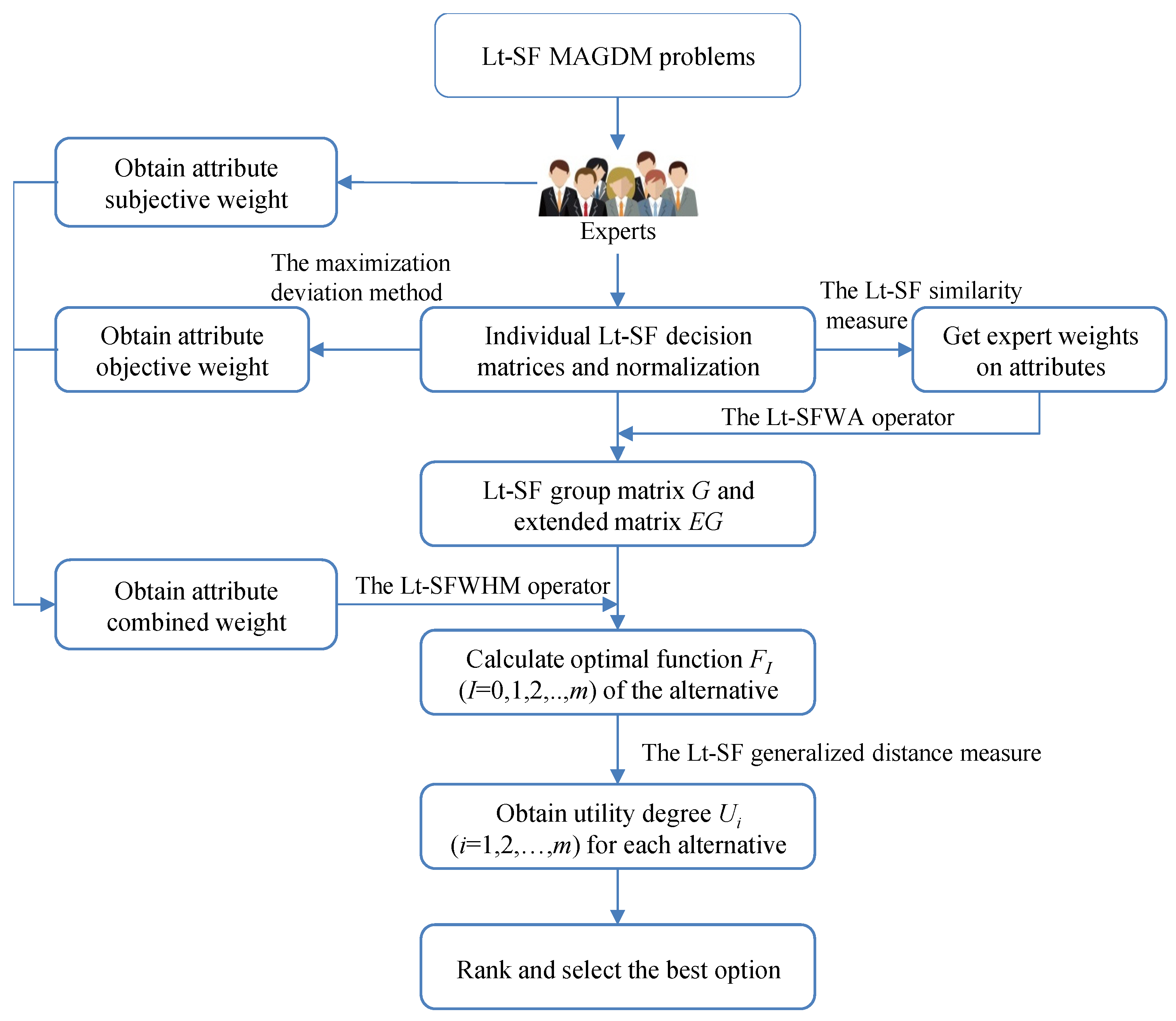
4. A New Lt-SF MAGDM Model Based on Improved ARAS

The MAGDM problems with Lt-SFNs are described as the following: Suppose H = {h₁,h₂, …, h_m} is a finite alternative set, A = {a₁,a₂, …, a_n} is an attribute set, and the attribute weight vector is W = {w₁,w₂, …, w_n}^T, $\sum _{j=1}^n{w}_j=1, w_j\in \left[0,1\right]$. E = {e₁, e₂, …, e_p} is a group of experts. As different experts possess different types of knowledge, experience, and in different industries, different weights are assigned to the corresponding attributes of different experts, but the same weight is not assigned to all attributes, so more reasonable decision-making results can be obtained. Let the weight of expert e_ε corresponding to attribute a_j be ${\omega }_{\epsilon }^{\left(j\right)}$, with $0\le {\omega }_{\epsilon }^{\left(j\right)}\le 1, \sum _{\epsilon =1}^p{\omega }_{\epsilon }^{\left(j\right)}=1$. The evaluation value given by expert e_ε (ε = 1, 2, …, p) of alternative h_i (i = 1, 2, …, m) under the attribute a_j (j = 1, 2, …, n) is represented by Lt-SFNs $d_{ij}^{\epsilon }=\left(s_{{\tau }_{ij}^{\epsilon }},s_{{\eta }_{ij}^{\epsilon }},s_{{\vartheta }_{ij}^{\epsilon }}\right)$, the constructed evaluation matrix is expressed as D^ε = [d_ij^ε]_m×n, (i = 1, 2, …, m; j = 1, 2, …, n; ε = 1, 2, …, p).

4.1. Calculate the Expert’s Weight Based on the Lt-SF Similarity Measure

Firstly, the decision matrix D^ε (ε = 1, 2, …, p) provided by the expert e_ε is transformed into an evaluation matrix for each attribute; that is, F^(j) (j = 1, 2, …, n), is denoted as follows:

$$F^{(j)}={[{\xi }_{\epsilon i}^{(j)}]}_{p\times m}=\begin{array}{cc}& \begin{array}{cccc}{h}_1& h_2& \cdots & h_m\end{array}\\ \begin{array}{c}{e}_1\\ e_2\\ ⋮\\ e_p\end{array}& \left[\begin{array}{cccc}{\xi }_{11}^{(j)}& {\xi }_{12}^{(j)}& \cdots & {\xi }_{1m}^{(j)}\\ {\xi }_{21}^{(j)}& {\xi }_{22}^{(j)}& \cdots & {\xi }_{2m}^{(j)}\\ ⋮& ⋮& \ddots & ⋮\\ {\xi }_{p1}^{(j)}& {\xi }_{p2}^{(j)}& \cdots & {\xi }_{pm}^{(j)}\end{array}\right]\end{array}$$

where ${\xi }_{\epsilon i}^{(j)}$ is equivalent to d_ij^ε.

For the matrix F^(j), the evaluation mean value of the alternative h_i with respect to the attribute a_j is ${\widehat{\xi }}_i^{(j)}=\left(s_{{\widehat{\tau }}_i^{(j)}},s_{{\widehat{\eta }}_i^{(j)}},s_{{\widehat{\vartheta }}_i^{(j)}}\right)$.

$${\widehat{\tau }}_i^{(j)}=\frac{1}{p}{\displaystyle \sum _{\epsilon =1}^p{\tau }_{\epsilon i}^{(j)}}, {\widehat{\eta }}_i^{(j)}=\frac{1}{p}{\displaystyle \sum _{\epsilon =1}^p{\eta }_{\epsilon i}^{(j)}}, {\widehat{\vartheta }}_i^{(j)}=\frac{1}{p}{\displaystyle \sum _{\epsilon =1}^p{\vartheta }_{\epsilon i}^{(j)}}$$

(17)

As for the alternative h_i ∈ H, the Lt-SF similarity measure is $si{m}_{\epsilon i}^{(j)}$ between ${\xi }_{\epsilon i}^{(j)}$ and ${\widehat{\xi }}_i^{(j)}$ based on Equation (8). For attribute a_j ∈ A, the similarity matrix S^(j) can be constructed by using the TSUL similarity measure $si{m}_{\epsilon i}^{(j)}$.

$$S^{(j)}={[si{m}_{\epsilon i}^{(j)}]}_{p\times m}=\begin{array}{cc}& \begin{array}{cccc}{h}_1& h_2& \cdots & h_m\end{array}\\ \begin{array}{c}{e}_1\\ e_2\\ ⋮\\ e_p\end{array}& \left[\begin{array}{cccc}si{m}_{11}^{(j)}& si{m}_{12}^{(j)}& \cdots & si{m}_{1m}^{(j)}\\ si{m}_{21}^{(j)}& si{m}_{22}^{(j)}& \cdots & si{m}_{2m}^{(j)}\\ ⋮& ⋮& \ddots & ⋮\\ si{m}_{p1}^{(j)}& si{m}_{p2}^{(j)}& \cdots & si{m}_{pm}^{(j)}\end{array}\right]\end{array}$$

(18)

Based on the similarity matrix S^(j), we can apply Equation (19) to obtain the overall similarity degree of expert e_ε with respect to attribute a_j ∈ A.

$${\gamma }_{\epsilon }^{(j)}={\displaystyle \sum _{i=1}^{m}si{m}_{\epsilon i}^{(j)}}$$

(19)

Lastly, the weight of expert e_k on the attribute a_j ∈ A can be obtained as below:

$${\omega }_{\epsilon }^{(j)}=\frac{{\gamma }_{\epsilon }^{(j)}}{{\displaystyle {\sum }_{\epsilon =1}^p{\gamma }_{\epsilon }^{(j)}}}$$

(20)

Obviously, $0\le {\omega }_{\epsilon }^{\left(j\right)}\le 1, \sum _{\epsilon =1}^p{\omega }_{\epsilon }^{\left(j\right)}=1$.

4.2. A Method for the Combined Attribute Weight

4.2.1. Calculate Objective Weight Based on the Maximization Deviation Method

When attribute weight information is completely unknown, the uncertainty of the attribute weight can affect the final ranking result of alternatives. Generally, if there is a small difference between the attribute values r_ij (i = 1, 2, …, m; j = 1, 2, …, n) in attribute a_j of all alternatives, it means that attribute a_j is of low importance in the ranking of all alternatives, and a small weight to this attribute can be assigned. Otherwise, a larger weight is assigned. Therefore, this paper can adopt the maximization deviation method [57] to obtain the objective attribute weight vector.

For attribute a_j ∈ A, the deviation of alternative h_i to all other alternatives h_l (l = 1, 2, …, m, l ≠ i) can be expressed as:

$$D_{ij}(w^o)={\displaystyle \sum _{l=1}^m{D}_{\phi }(r_{ij},r_{lj})w_j^o}$$

(21)

D_j(w^o) represents the deviation value from all alternatives to other alternatives for attribute a_j ∈ A, so it can be expressed as:

$$D_j(w^o)={\displaystyle \sum _{i=1}^m{D}_{ij}(w^o)=}{\displaystyle \sum _{i=1}^m{\displaystyle \sum _{l=1}^m{D}_{\phi }(r_{ij},r_{lj})w_j^o}}$$

(22)

where $D_{\phi }(r_{ij},r_{lj})$ represents the Lt-SF generalized distance measure between r_ij and r_lj, which can be obtained from Equation (7).

Therefore, we can build a linear mathematical model that maximizes all deviations for all attributes to assign the objective weight vector W^o, as follows:

$$\{\begin{array}{l}Max D(w^o)={\displaystyle \sum _{j=1}^n{\displaystyle \sum _{i=1}^m{D}_{ij}(w^o)}}={\displaystyle \sum _{j=1}^n{\displaystyle \sum _{i=1}^m{\displaystyle \sum _{l=1}^m{D}_{\phi }(r_{ij},r_{lj})w_j^o}}}\\ s.t.{\displaystyle \sum _{j=1}^n{(w_j^o)}^2}=1,0\le w_j^o\le 1\end{array}$$

(23)

To solve Equation (23), we apply the Lagrange function with Lagrange multiplierλ. Then we have

$$L(w_j^o,\lambda )={\displaystyle \sum _{j=1}^n{\displaystyle \sum _{i=1}^m{\displaystyle \sum _{l=1}^m{D}_{\phi }(r_{ij},r_{lj})w_j^o}+\lambda \left({\displaystyle \sum _{j=1}^n{(w_j^o)}^2}-1\right)}}$$

Let

$$\{\begin{array}{l}\frac{\partial L(w_j^o,\lambda )}{\partial w_j^o}={\displaystyle \sum _{i=1}^m{\displaystyle \sum _{l=1}^m{D}_{\phi }(r_{ij},r_{lj})w_j^o}+2\lambda w_j^o}=0\\ \frac{\partial L(w_j^o,\lambda )}{\partial \lambda }={\displaystyle \sum _{j=1}^n{(w_j^o)}^2}-1=0\end{array}$$

Thus, we can obtain a formula for the optimal weight of the attributes as follows:

$$w_j^{*}=\frac{{\displaystyle \sum _{i=1}^m{\displaystyle \sum _{l=1}^m{D}_{\phi }(r_{ij},r_{lj})}}}{\sqrt{{\displaystyle \sum _{j=1}^n{\left({\displaystyle \sum _{i=1}^m{\displaystyle \sum _{l=1}^m{D}_{\phi }(r_{ij},r_{lj})}}\right)}^2}}}$$

By normalizing w_j*, we obtain the attribute weight $w_j^o$ (j = 1, 2, …, n).

$$w_j^o=\frac{{\displaystyle \sum _{i=1}^m{\displaystyle \sum _{l=1}^m{D}_{\phi }(r_{ij},r_{lj})}}}{{\displaystyle \sum _{j=1}^n{\displaystyle \sum _{i=1}^m{\displaystyle \sum _{l=1}^m{D}_{\phi }(r_{ij},r_{lj})}}}}$$

(24)

4.2.2. Calculate Attribute Subjective Weight

Firstly, the expert e_ε (ε = 1, 2, …, p) gives the evaluation of attribute a_j (j = 1, 2, …, n) importance to form the individual importance matrix J^ε.

$$J^{\epsilon }={(J_1^{\epsilon },J_2^{\epsilon },\dots ,J_n^{\epsilon })}_{1\times n}^T$$

(25)

where the ‘importance evaluation’ value is expressed by the Lt-SFN, i.e., $J_j^{\epsilon }=\left(s_{{\tau }_j^{\epsilon }},s_{{\eta }_j^{\epsilon }},s_{{\vartheta }_j^{\epsilon }}\right)$.

Then, the importance evaluation of each expert for attribute a_j is aggregated, and the Lt-SFWA operator is used to obtain as below.

$${\varpi }_j=Lt-SFWA(J_j^1,J_j^2,\dots ,J_j^p)=\underset{\epsilon =1}{\overset{p}{\oplus }}{\omega }_{\epsilon }^{(j)}{J}_j^{\epsilon }=\left(s_{k{\left(1-{\displaystyle \prod _{\epsilon =1}^p{\left(1-({\tau }_j^{\epsilon }/k{)}^q\right)}^{{\omega }_{\epsilon }^{(j)}}}\right)}^{1/q}},s_{k{\displaystyle \prod _{\epsilon =1}^p{\left(\frac{{\eta }_j^{\epsilon }}{k}\right)}^{{\omega }_{\epsilon }^{(j)}}}},s_{k{\displaystyle \prod _{\epsilon =1}^p{\left(\frac{{\vartheta }_j^{\epsilon }}{k}\right)}^{{\omega }_{\epsilon }^{(j)}}}}\right)$$

(26)

Lastly, we calculate the score function sc(ϖ_j) by Equation (3), and obtain the subjective weight of attribute a_j by using the following Equation (27).

$$w_j^s=\frac{f^{\ast }(sc({\varpi }_j))}{{\displaystyle {\sum }_{j=1}^n{f}^{\ast }(sc({\varpi }_j))}}$$

(27)

where f*(.) is the linguistic scale function [58,59]; it is used to convert linguistic terms to real numbers.

4.2.3. Determine the Combined Attribute Weight

Equation (28) is used to calculate the combined weight w_j^c (j = 1, 2, …, n):

$$w_j^c=\frac{\sqrt{w_j^s{w}_j^o}}{{\displaystyle {\sum }_{j=1}^n\sqrt{w_j^s{w}_j^o}}}$$

(28)

4.3. Rank the Alternatives by Lt-SF ARAS

The existing ARAS methods cannot handle Lt-SFNs. In this sub-section, the ARAS method is extended to the Lt-SF context. The decision process is as below (graphical framework is given in Figure 2):

Step 1: the Lt-SF evaluation matrix D^ε = [d_ij^ε]_m×n, is constructed and normalized to the normalized decision matrix R^ε = [r_ij^ε]_m×n.

$$r_{ij}^{\epsilon }=\{\begin{array}{c}{d}_{ij}^{\epsilon }=\left(s_{{\tau }_{ij}^{\epsilon }},s_{{\eta }_{ij}^{\epsilon }},s_{{\vartheta }_{ij}^{\epsilon }}\right);h_j\in {\mathsf{\Psi }}_1\\ {(d_{ij}^{\epsilon })}^c=\left(s_{{\vartheta }_{ij}^{\epsilon }},s_{{\eta }_{ij}^{\epsilon }},s_{{\tau }_{ij}^{\epsilon }}\right);h_j\in {\mathsf{\Psi }}_2\end{array}$$

(29)

where ${(d_{ij}^{\epsilon })}^c$ is the complement set of Lt-SFN $d_{ij}^{\epsilon }$, Ψ₁ and Ψ₂ indicate the benefit and cost attributes, respectively.

Step 2: the expert weight determination method in Section 4.1 is utilized to calculate the weight of experts for different attributes ${\omega }_{\epsilon }^{\left(j\right)}$.

Step 3: the evaluation information of each expert is aggregated by utilizing the Lt-SFWA operator to obtain the Lt-SF group decision matrix $G={[g_{ij}]}_{m\times n}$.

$$g_{ij}=Lt-SFWA(r_{ij}^1,r_{ij}^2,\dots ,r_{ij}^p)=\left(s_{k{\left(1-{\displaystyle \prod _{\epsilon =1}^p{\left(1-({\tau }_{ij}^{\epsilon }/k{)}^q\right)}^{{\omega }_{\epsilon }^{(j)}}}\right)}^{1/q}},s_{k{\displaystyle \prod _{\epsilon =1}^p{\left(\frac{{\eta }_{ij}^{\epsilon }}{k}\right)}^{{\omega }_{\epsilon }^{(j)}}}},s_{k{\displaystyle \prod _{\epsilon =1}^p{\left(\frac{{\vartheta }_{ij}^{\epsilon }}{k}\right)}^{{\omega }_{\epsilon }^{(j)}}}}\right)$$

(30)

Then, we obtain the Lt-SF extended group decision matrix EG according to Equation (31).

$$EG=\begin{array}{cc}& \begin{array}{cccc}{a}_1 & a_2 & \dots & a_n\end{array}\\ \begin{array}{c}{h}_0\\ h_1\\ ⋮\\ h_m\end{array}& \left[\begin{array}{c}\begin{array}{cccc}{g}_{01}& g_{02}& \dots & g_{0n}\end{array}\\ \begin{array}{cccc}{g}_{11}& g_{12}& \dots & g_{1n}\end{array}\\ \begin{array}{cccc}⋮& ⋮& \ddots & ⋮\end{array}\\ \begin{array}{cccc}{g}_{m1}& g_{m2}& \dots & g_{mn}\end{array}\end{array}\right]\end{array}$$

(31)

where h₀ = (g₀₁, g₀₂,…, g_0n)^T is the ideal solution, which is determined by $g_{0j}=\max (g_{ij})=\left(s_{\underset{i}{\max }{\tau }_{ij}},s_{\underset{i}{\min }{\eta }_{ij}},s_{\underset{i}{\min }{\vartheta }_{ij}}\right)$.

Step 4: we apply the combined attribute weight determination method in Section 4.2 to obtain the combined attribute weight w_j^c (j = 1, 2, …, n).

Step 5: We have the optimal function F_I (I = 0, 1, 2, …, m) of the alternative according to the Lt-SFWHM operator (Equation (16)). For the attribute hierarchy system with a complex hierarchy and the correlation structure, a large number of associated attributes can cause complex calculations in the process of evaluating the value aggregation. Thus, this paper designs the aggregation process as shown in Figure 3. This paper first aggregates the assessment information δ_jl^I of the sub-attribute layer to form the evaluation value δ_j^I of the attribute layer and then aggregates the attribute layer to form the optimal function F_I (I = 0, 1, 2,…m) of the alternative.

Step 6: we use the Lt-SF generalized distance measure (Equation (7)) to calculate the utility degree $U_i=D_{\phi }(F_i,F_0)$ (i = 1, 2, …, m) of each alternative, which indicates the deviation between the alternative and the ideal solution.

Step 7: the alternatives are ranked according to an ascending order U_i, and then the optimal alternative with the smallest value of U_i is selected.

5. A Case Study: SCS Selection in the Power Battery Industry

In this segment, a practical decision-making problem of the SCS selection in the power battery industry is provided to test the proposed method in this paper.

In China, the development of new energy vehicles is strong. By the first half of 2021, the number of new energy vehicles in China was 6.03 million, accounting for 2.06% of the total number of vehicles. With the development of China’s new energy vehicle industry, the power battery recycling after scrap increases each year. According to statistics by the Ministry of Commerce of China, the amount of waste batteries recycled (except lead acid) in China increased each year from 2013 to 2020; in 2020, 274,000 tons of spent power batteries were recycled (except lead acid), as shown in Figure 4.

Due to the COVID-19 epidemic and the shortage of raw material resources, more power battery manufacturers are choosing to recycle precious metals from spent power batteries as renewable materials of the anode and ternary materials. At present, driven by government policies and market laws, many power battery manufacturers are laying out the resource utilizations of power batteries. The SCS selection of power batteries is an important enterprise strategy.

A power battery manufacturer selected a resource recycling company as a SCS of power battery recycling materials. The decision problem is described below:

(1)

A panel of three experts E = {e₁, e₂, e₃} was established, including a production manager, a supply chain manager, and a professor who had at least ten years of knowledge and work experience in this field.

(2)

After the primary selection, five resource recycling company were retained as candidate SCSs for further evaluation: H = {h₁, h₂, …, h₅}.

(3)

Through discussion, the decision-making committee determined the attribute hierarchy system shown in

Table 1. Attribute system for SCS selection in the power battery industry.

Attributes	Sub-Attributes	Types	References
a1: Economy	a11: financial capacity	B	Liu et al. [16]; Alrasheedi et al. [60]; Yu et al. [61]; Rashidi et al. [62]
	A12: quality	B	Jain et al. [63]; Ecer et al. [64]; Li et al. [65]; Khan et al. [66]
	A13: technical capacity	B	Jia et la. [67]; Memari et al. [68]; Luthra et al. [69];
	a14: cost or price	C	Yu et al. [61]; Rashidi et al. [62]; Mishra et al. [70]
	a15: timely delivery	B	Kannan et al. [15]; Rashidi et al. [62]; Jia et la. [67]; Stevič et al. [71]
a2: Circularity	a21: using clean and green technologies	B	Kannan et al. [15]; Alavi et al. [18]; Li et al. [65]; Khan et al. [66]
	a22: energy consumption	C	Alavi et al. [18]; Luthra et al. [69]; Yu et al. [72];Liu et al. [73]
	a23: environmental management system	B	Luthra et al. [69];Yu et al. [61]; Rashidi et al. [62]; Mishra et al. [74]; Chen et al. [75]
	a24: reverse logistics or recycling network	B	Stevič et al. [71]; Yu et al. [72]; Liu et al. [73];
a3: Society	a31: work safety and health	B	Jia et la. [67]; Li et al. [65]; Stevič et al. [71]; Chen et al. [75]
	a32: impact on local communities	B	Rashidi et al. [62]; Li et al. [65]; Zhou et al. [76]; Govindan et al. [77]
	a33: staff training	B	Rashidi et al. [62]; Ecer et al. [64]; Li et al. [65]; Govindan et al. [78]
	a34: rights/guarantees of employees and stakeholders	B	Kannan et al. [15]; Alrasheedi et al. [60]; Ecer et al. [64]; Luthra et al. [69];

and used it to evaluate options.

(4)

Each expert used an LTS, i.e., S = {s₀, s₁, s₂, s₃, s₄, s₅, s₆} = {extremely low, very low, low, medium, high, very high, extremely high}, to evaluate the five alternatives. The evaluation values are shown in

Table 2. Initial linguistic evaluation information given by three experts (q = 3).

Attributes	Sub-Attributes	Experts	h1	h2	h3	h4	h5
a1	a11	e1	(s4,s3,s5)	(s5,s3,s3)	(s6,s4,s3)	(s5,s2,s4)	(s3,s3,s4)
		e2	(s2,s4,s2)	(s3,s1,s2)	(s2,s2,s5)	(s4,s3,s1)	(s4,s2,s3)
		e3	(s3,s2,s4)	(s4,s1,s4)	(s5,s3,s2)	(s4,s3,s4)	(s5,s1,s2)
	a12	e1	(s5,s2,s2)	(s5,s3,s2)	(s5,s2,s1)	(s6,s3,s4)	(s5,s3,s1)
		e2	(s6,s2,s1)	(s3,s5,s1)	(s6,s1,s1)	(s4,s2,s3)	(s3,s3,s5)
		e3	(s4,s2,s3)	(s3,s3,s4)	(s4,s4,s3)	(s5,s2,s1)	(s5,s3,s2)
	a13	e1	(s3,s1,s4)	(s5,s3,s1)	(s4,s1,s1)	(s6,s3,s3)	(s5,s1,s3)
		e2	(s5,s2,s4)	(s4,s3,s3)	(s4,s5,s2)	(s4,s3,s2)	(s3,s3,s1)
		e3	(s4,s1,s4)	(s5,s4,s5)	(s5,s2,s4)	(s5,s1,s1)	(s6,s3,s4)
	a14	e1	(s4,s3,s3)	(s3,s1,s0)	(s4,s4,s2)	(s1,s3,s5)	(s2,s6,s4)
		e2	(s2,s5,s4)	(s4,s2,s4)	(s2,s3,s4)	(s4,s2,s5)	(s3,s3,s4)
		e3	(s2,s6,s4)	(s3,s3,s2)	(s4,s2,s1)	(s3,s1,s5)	(s4,s4,s2)
	a15	e1	(s4,s4,s3)	(s2,s2,s1)	(s4,s2,s3)	(s5,s1,s1)	(s6,s4,s2)
		e2	(s5,s4,s3)	(s4,s1,s4)	(s5,s5,s1)	(s5,s3,s3)	(s4,s1,s5)
		e3	(s4,s3,s3)	(s5,s3,s1)	(s6,s3,s2)	(s4,s4,s1)	(s5,s5,s1)
a2	a21	e1	(s2,s5,s3)	(s4,s3,s4)	(s4,s2,s5)	(s4,s1,s3)	(s5,s3,s3)
		e2	(s6,s1,s4)	(s3,s4,s5)	(s4,s3,s3)	(s5,s3,s1)	(s3,s4,s3)
		e3	(s5,s2,s2)	(s4,s2,s3)	(s5,s5,s1)	(s5,s4,s4)	(s5,s4,s2)
	a22	e1	(s2,s3,s5)	(s4,s1,s4)	(s2,s1,s5)	(s1,s3,s5)	(s2,s3,s3)
		e2	(s1,s4,s0)	(s5,s2,s4)	(s3,s2,s4)	(s3,s1,s6)	(s5,s3,s2)
		e3	(s4,s2,s5)	(s3,s3,s4)	(s4,s4,s2)	(s2,s5,s5)	(s1,s4,s4)
	a23	e1	(s6,s3,s3)	(s5,s1,s2)	(s5,s4,s4)	(s6,s1,s2)	(s6,s2,s4)
		e2	(s2,s4,s3)	(s4,s1,s1)	(s4,s5,s1)	(s5,s4,s3)	(s4,s5,s2)
		e3	(s4,s2,s3)	(s3,s2,s3)	(s6,s4,s2)	(s5,s5,s1)	(s4,s3,s4)
	a24	e1	(s1,s3,s6)	(s4,s3,s1)	(s6,s2,s3)	(s4,s3,s2)	(s3,s3,s3)
		e2	(s4,s2,s2)	(s5,s2,s1)	(s3,s3,s4)	(s4,s4,s1)	(s2,s4,s2)
		e3	(s3,s3,s2)	(s4,s3,s3)	(s5,s2,s3)	(s5,s1,s4)	(s4,s2,s2)
a3	a31	e1	(s3,s3,s1)	(s4,s2,s3)	(s3,s2,s2)	(s4,s1,s2)	(s3,s5,s1)
		e2	(s4,s2,s3)	(s3,s2,s1)	(s5,s3,s3)	(s3,s1,s1)	(s4,s2,s4)
		e3	(s4,s2,s5)	(s5,s4,s3)	(s4,s1,s6)	(s5,s3,s4)	(s5,s2,s5)
	a32	e1	(s5,s3,s2)	(s2,s1,s5)	(s4,s3,s3)	(s5,s2,s2)	(s4,s5,s3)
		e2	(s3,s1,s4)	(s4,s4,s2)	(s5,s3,s5)	(s6,s3,s1)	(s5,s1,s4)
		e3	(s5,s6,s1)	(s3,s3,s1)	(s4,s4,s2)	(s4,s2,s1)	(s5,s3,s3)
	a33	e1	(s5,s2,s4)	(s3,s6,s2)	(s3,s1,s4)	(s4,s1,s1)	(s5,s3,s5)
		e2	(s5,s3,s3)	(s5,s2,s1)	(s4,s3,s6)	(s5,s3,s2)	(s4,s4,s2)
		e3	(s4,s1,s2)	(s4,s3,s1)	(s5,s3,s3)	(s4,s2,s2)	(s4,s1,s3)
	a34	e1	(s6,s2,s4)	(s4,s3,s3)	(s4,s2,s3)	(s5,s2,s4)	(s5,s5,s2)
		e2	(s4,s3,s3)	(s4,s2,s1)	(s5,s1,s5)	(s4,s3,s2)	(s5,s3,s4)
		e3	(s5,s3,s4)	(s5,s2,s2)	(s4,s4,s5)	(s5,s3,s3)	(s4,s3,s3)

, in which all the values are expressed as Lt-SFNs. The Lt-SFN can be given directly by experts or converted from linguistic terms.

5.1. Decision Process

Step 1: In the attribute hierarchy system, a₁₄ and a₂₂ are cost attributes; Equation (29) is utilized for normalization. For example, the evaluation value of expert e₁ on attribute a₁₄ is $d_{14}^1=(s_4,s_3,s_3)$, and the normalized evaluation value is $r_{14}^1=(s_3,s_3,s_4)$.

Step 2: We can obtain the similarity matrix S^(j) by using Equations (8), (18), and (19). For example, the similarity matrix S⁽¹¹⁾ with regard to sub-attribute a₁₁ is

$$S^{(11)}=\begin{array}{cc}& \begin{array}{ccc}{h}_1 & h_2 & \begin{array}{ccc}{h}_3 & h_4 & h_5\end{array}\end{array}\\ \begin{array}{c}{e}_1\\ e_2\\ e_3\end{array}& \left[\begin{array}{c}\begin{array}{ccc}0.722& 0.792& \begin{array}{ccc}0.611& 0.800& 0.863\end{array}\end{array}\\ \begin{array}{ccc}0.773& 0.791& \begin{array}{ccc}0.619& 0.839& 0.973\end{array}\end{array}\\ \begin{array}{ccc}0.894& 0.927& \begin{array}{ccc}0.804& 0.903& 0.849\end{array}\end{array}\end{array}\right]\end{array}$$

Then, we can calculate the expert weight value of the sub-attribute by Equation (20).

${\omega }_1^{11}=0.312,{\omega }_2^{11}=0.329,{\omega }_3^{11}=0.360$; ${\omega }_1^{12}=0.347,{\omega }_2^{12}=0.313,{\omega }_3^{12}=0.340$;

${\omega }_1^{13}=0.345,{\omega }_2^{13}=0.322,{\omega }_3^{13}=0.334$; ${\omega }_1^{14}=0.317,{\omega }_2^{14}=0.342,{\omega }_3^{14}=0.342$;

${\omega }_1^{15}=0.334,{\omega }_2^{15}=0.327,{\omega }_3^{15}=0.339$; ${\omega }_1^{21}=0.344,{\omega }_2^{21}=0.330,{\omega }_3^{21}=0.326$;

${\omega }_1^{22}=0.351,{\omega }_2^{22}=0.329,{\omega }_3^{22}=0.321$; ${\omega }_1^{23}=0.322,{\omega }_2^{23}=0.338,{\omega }_3^{23}=0.341$;

${\omega }_1^{24}=0.323,{\omega }_2^{24}=0.333,{\omega }_3^{24}=0.344$; ${\omega }_1^{31}=0.348,{\omega }_2^{31}=0.363,{\omega }_3^{31}=0.288$;

${\omega }_1^{32}=0.350,{\omega }_2^{32}=0.313,{\omega }_3^{32}=0.338$; ${\omega }_1^{33}=0.324,{\omega }_2^{33}=0.336,{\omega }_3^{33}=0.340$;

${\omega }_1^{34}=0.320,{\omega }_2^{34}=0.330,{\omega }_3^{34}=0.350$.

Step 3: The Lt-SFWA operator (Equation (30)) is applied to aggregate individual evaluation information, constructs the Lt-SF group decision matrix G, and then determines the Lt-SF extended group decision matrix EG by Equation (31); the results are listed in

Table 3. Lt-SF extended group decision matrix EG.

		h1	h2	h3	h4	h5	h0
a1	a11	(s3.212,s2.850,s3.415)	(s4.195,s1.408,s2.912)	(s5.077,s2.872,s3.066)	(s4.391,s2.644,s2.537)	(s4.265,s1.768,s2.836)	(s5.077,s1.408,s2.537)
	a12	(s5.228,s2.000,s1.847)	(s4.024,s3.521,s2.037)	(s5.228,s2.037,s1.452)	(s5.286,s2.302,s2.282)	(s4.612,s3.000,s2.096)	(s5.286,s2.000,s1.452)
	a13	(s4.198,s1.250,s4.000)	(s4.747,s3.302,s2.436)	(s4.415,s2.115,s1.985)	(s5.278,s2.080,s1.825)	(s5.166,s2.055,s2.319)	(s5.278,s1.250,s1.825)
	a14	(s3.751,s4.527,s2.491)	(s2.960,s1.845,s3.310)	(s2.965,s2.861,s3.157)	(s5.000,s1.794,s2.338)	(s3.583,s4.122,s2.911)	(s5.000,s1.794,s2.338)
	a15	(s4.407,s3.628,s3.000)	(s4.125,s1.830,s1.573)	(s5.264,s3.096,s1.826)	(s4.732,s2.291,s1.432)	(s5.262,s2.743,s2.133)	(s5.264,s1.830,s1.432)
a2	a21	(s5.085,s2.182,s2.890)	(s3.740,s2.890,s3.920)	(s4.406,s3.082,s2.500)	(s4.728,s2.257,s2.294)	(s4.589,s3.623,s2.629)	(s5.085,s2.182,s2.294)
	a22	(s4.481,s2.895,s1.989)	(s4.000,s1.786,s3.925)	(s4.154,s1.959,s2.854)	(s5.434,s2.463,s1.792)	(s3.223,s3.290,s2.164)	(s5.434,s1.786,s1.792)
	a23	(s4.829,s2.879,s3.000)	(s4.201,s1.266,s1.817)	(s5.264,s4.313,s1.978)	(s5.426,s2.763,s1.811)	(s5.019,s3.129,s3.165)	(s5.426,s1.266,s1.811)
	a24	(s3.175,s2.621,s2.851)	(s4.414,s2.621,s1.459)	(s5.140,s2.289,s3.302)	(s4.426,s2.262,s2.015)	(s3.249,s2.872,s2.280)	(s5.140,s2.262,s1.459)
a3	a31	(s3.724,s2.303,s2.371)	(s4.143,s2.443,s2.012)	(s4.247,s1.898,s3.182)	(s4.143,s1.373,s1.899)	(s4.153,s2.633,s2.633)	(s4.247,s1.373,s1.899)
	a32	(s4.613,s2.689,s1.966)	(s3.201,s2.236,s2.180)	(s4.392,s3.306,s3.069)	(s5.228,s2.270,s1.274)	(s4.723,s2.544,s3.282)	(s5.228,s2.236,s1.274)
	a33	(s4.732,s1.811,s2.870)	(s4.229,s3.277,s1.252)	(s4.233,s2.101,s4.158)	(s4.418,s1.831,s1.597)	(s4.405,s2.276,s4.204)	(s4.732,s1.811,s1.252)
	a34	(s5.242,s2.635,s3.637)	(s4.432,s2.277,s1.811)	(s4.411,s2.027,s4.246)	(s4.740,s2.635,s2.877)	(s4.723,s3.533,s2.898)	(s5.242,s2.027,s1.811)

.

Step 4: According to the attribute hierarchy system and Section 4.2, we first calculate the weight of the sub-attribute, and then obtain the attribute weight.

(1)

Based on the Lt-SF group decision G, we utilize Equation (24) to calculate the sub-attribute weight vector as:

W^o = (0.068,0.060,0.070,0.103,0.083,0.064,0.095,0.103,0.084,0.035,0.083,0.072,0.082)^T

(2)

Meanwhile, the subjective importance of the sub-attribute is evaluated by three experts and expressed by Lt-SFNs. See

Table 4. The evaluation of sub-attribute importance by experts.

Experts	a1					a2
	a11	a12	a13	a14	a15	a21	a22
e1	(s4,s2,s2)	(s5,s3,s1)	(s4,s1,s1)	(s5,s2,s2)	(s5,s3,s2)	(s4,s1,s2)	(s4,s3,s1)
e2	(s5,s2,s2)	(s6,s1,s3)	(s5,s2,s3)	(s6,s4,s4)	(s5,s3,s1)	(s4,s3,s2)	(s4,s2,s1)
e3	(s5,s2,s1)	(s6,s2,s4)	(s5,s3,s3)	(s6,s3,s2)	(s5,s5,s1)	(s4,s3,s1)	(s4,s4,s5)
Experts	a2		a3
	a23	a24	a31	a32	a33	a34
e1	(s3,s1,s1)	(s6,s1,s3)	(s4,s2,s2)	(s4,s3,s1)	(s3,s4,s2)	(s2,s2,s4)
e2	(s4,s3,s5)	(s4,s1,s1)	(s5,s4,s3)	(s2,s5,s3)	(s4,s3,s4)	(s2,s3,s4)
e3	(s4,s2,s2)	(s6,s4,s3)	(s3,s3,s4)	(s2,s2,s5)	(s4,s3,s2)	(s3,s1,s1)

.

This paper uses Equation (26) to aggregate the importance evaluation of each sub-attribute; Equation (27) is used to obtain the sub-attribute subjective weight as

W^s = (0.077,0.065,0.077,0.064,0.075,0.082,0.081,0.082,0.068,0.078,0.084,0.082,0.085)^T.

(3)

Lastly, the weight value of the sub-attribute from Equation (28) is

W^c = (0.073,0.063,0.074,0.082,0.080,0.073,0.089,0.093,0.076,0.053,0.084,0.077,0.084)^T.

Thus, we can easily obtain that the weights of attributes a₁, a₂, a₃ are 0.372, 0.330, and 0.298, respectively.

Step 5: The Lt-SFWHM operator (Equation (16)) (ς = ψ = 1) is used to aggregate the sub-attributes under each attribute, and then the Lt-SFWHM operator is used to aggregate each attribute again to obtain the alternative optimal function F_I, as shown in

Table 5. Results of aggregation using the Lt-SFWHM operator twice.

	h1	h2	h3	h4	h5	h0
a1	(s3.943,s3.780,s3.770)	(s3.793,s3.301,s3.343)	(s4.395,s3.416,s3.175)	(s4.642,s3.097,s2.986)	(s4.338,s3.607,s3.295)	(s4.863,s2.535,s2.802)
a2	(s4.125,s3.639,s3.727)	(s3.768,s3.342,s3.914)	(s4.393,s3.978,s3.723)	(s4.652,s3.457,s3.084)	(s3.774,s4.142,s3.593)	(s4.877,s3.048,s2.940)
a3	(s4.288,s3.461,s3.811)	(s3.689,s3.658,s2.991)	(s3.972,s3.446,s4.547)	(s4.301,s3.115,s3.130)	(s4.160,s3.831,s4.218)	(s4.526,s2.959,s2.750)
FI	(s3.670,s4.690,s4.796)	(s3.343,s4.563,s4.555)	(s3.802,s4.696,s4.887)	(s4.052,s4.405,s4.286)	(s3.653,s4.872,s4.780)	(s4.256,s4.141,s4.101)
Ui	0.214	0.144	0.234	0.071	0.247	-
Ranking	3	2	4	1	5	-

.

Step 6: The Lt-SF generalized distance measure (Equation (7)) (ϕ = 1) is employed to calculate the utility degree U_i of each alternative. The results are presented in Table 5.

Step 7: According to the utility degree U_i of each alternative in

Table 6. The results of the alternative ranking with different q’s.

q	U1	U2	U3	U4	U5	Rankings	The Best Option
3	0.214	0.144	0.234	0.071	0.247	h4 < h2 < h1 < h3 < h5	h4
4	0.187	0.128	0.213	0.058	0.221	h4 < h2 < h1 < h3 < h5	h4
5	0.159	0.111	0.189	0.047	0.194	h4<h2 < h1 < h3 < h5	h4
6	0.134	0.094	0.168	0.038	0.169	h4 < h2 < h1 < h3 < h5	h4
7	0.115	0.080	0.148	0.031	0.149	h4 < h2 < h1 < h3 < h5	h4
8	0.099	0.069	0.132	0.026	0.131	h4 < h2 < h1 < h5 < h3	h4
9	0.088	0.060	0.119	0.022	0.117	h4 < h2 < h1 < h5 < h3	h4
10	0.078	0.053	0.107	0.019	0.105	h4 < h2 < h1 < h5 < h3	h4

, the alternative is ranked as h₄ < h₂ < h₁ < h₃ < h₅. The smaller the better. Therefore, h₄ is the best option.

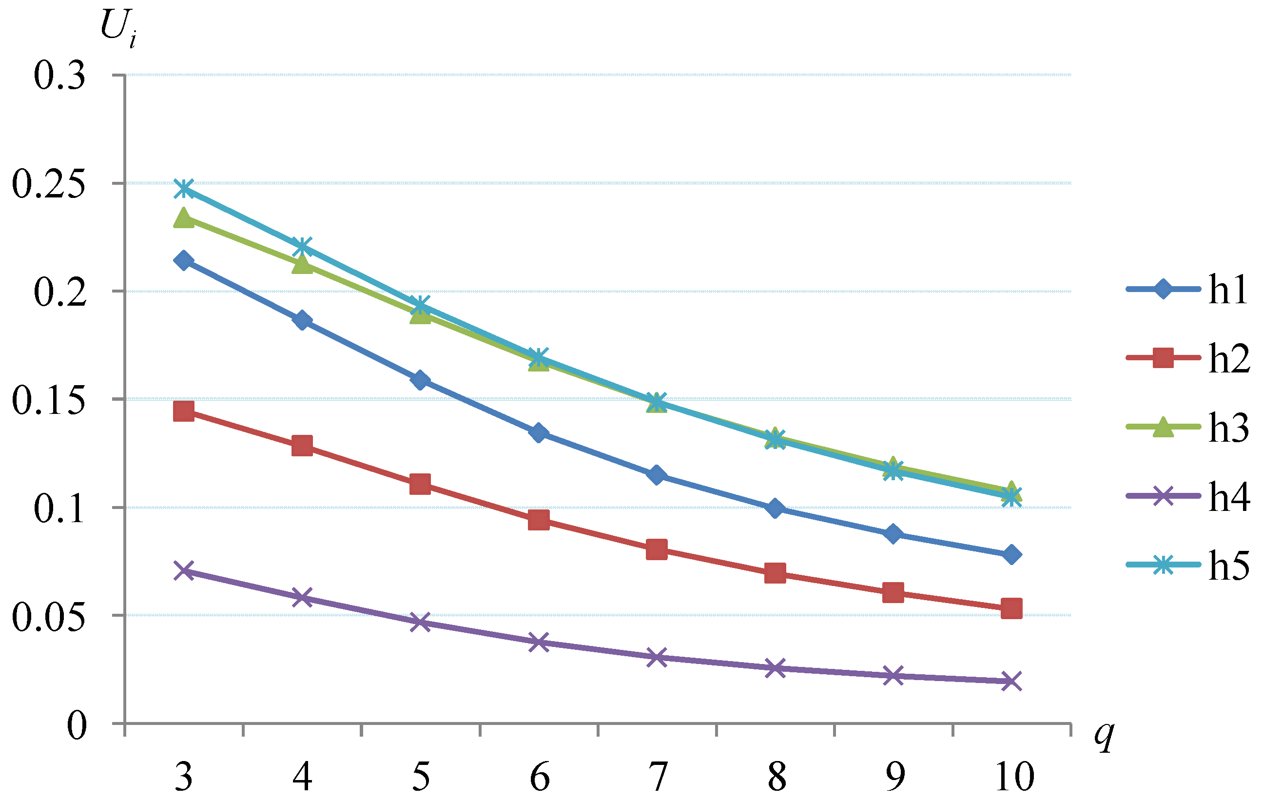
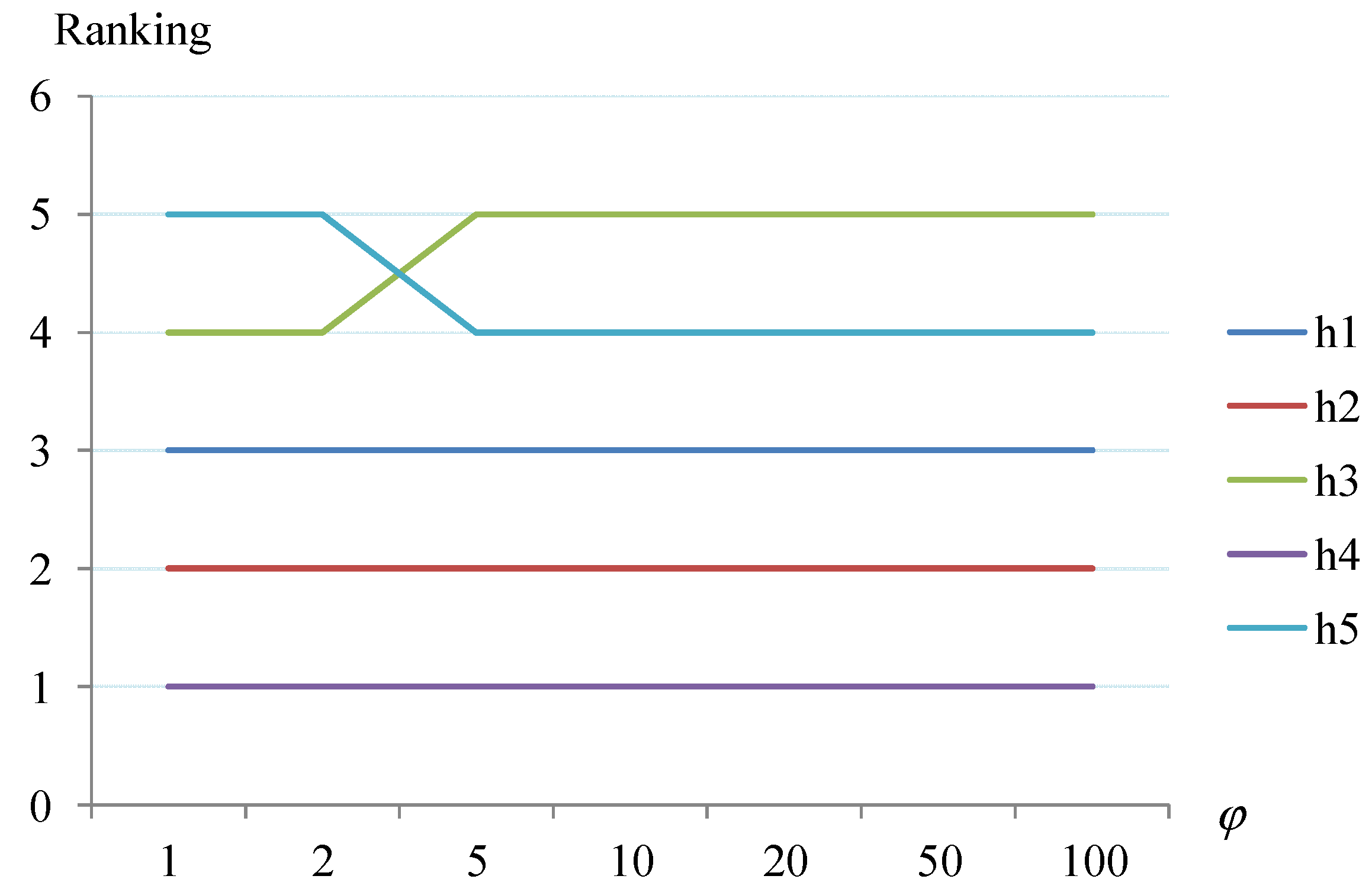
5.2. Sensitivity Analysis

The influences of different parameters q, ϕ, ς, and ψ on the decision results are analyzed in this sub-section. First, this article takes the value of parameter q ∈ [3, 10] and ranks the alternatives; the results are shown in Table 6 and Figure 4.

From Table 6 and Figure 5, the optimal utility function value U_i of each alternative decreases with the increase of the parameter q value on the whole. When taking the value in parameter q ∈ [3,10], according to the value of the optimal utility function of each alternative, the alternative ranking changes from h₄ < h₂ < h₁ < h₃ < h₅ to h₄ < h₂ < h₁ < h₅ < h₃. The ranking of alternatives h₅ and h₃ only changes slightly, but the optimal alternative is always h₄, and the sub-optimal alternative is h₁. Therefore, the influence of parameter q on the alternative ranking is relatively stable. This shows that the influence of the proposed method on parameter q is robust.

Next, we analyze the ranking of alternatives when the parameter ϕ takes different values. This paper takes the values of parameter ϕ as 1, 2, 5, 10, 20, 50, and 100 respectively, and obtains the optimal utility function value of each alternative; the results are presented in

Table 7. Alternative results for different parameters ϕ values.

ϕ	U1	U2	U3	U4	U5	The Best Option	The Worst Option
1	0.214	0.144	0.234	0.071	0.247	h4	h5
2	0.154	0.111	0.175	0.051	0.180	h4	h5
5	0.130	0.104	0.159	0.043	0.156	h4	h3
10	0.127	0.108	0.161	0.041	0.155	h4	h3
20	0.127	0.112	0.164	0.041	0.159	h4	h3
50	0.129	0.114	0.168	0.042	0.162	h4	h3
100	0.129	0.115	0.169	0.042	0.163	h4	h3

.

From Table 7, when the parameter ϕ takes different values, the optimal alternative is h₄, but the worst alternative changes from h₅ to h₃. Thus, we can see from Figure 6 that with the change of parameter ϕ, the ranking of each alternative is relatively stable. This shows that the influence of the parameter ϕ change on the proposed method is robust.

Finally, parameters ς and ψ play important roles in the final result of the alternative. We give different values to the parameters ς and ψ in step 5, and we can obtain different ranking results; see

Table 8. Alternative ranking results for different parameters, ς,ψ.

ς, ψ	U1	U2	U3	U4	U5	Rankings
0, 1	0.281	0.083	0.348	0.132	0.363	h2 < h4 < h1 < h3 < h5
1, 0	0.216	0.190	0.181	0.128	0.210	h4 < h3 < h2 < h5 < h1
0.5, 0.5	0.264	0.182	0.287	0.090	0.302	h4 < h2 < h1 < h3 < h5
1, 1	0.214	0.144	0.234	0.071	0.247	h4 < h2 < h1 < h3 < h5
1, 3	0.172	0.139	0.209	0.061	0.216	h4 < h2 < h1 < h3 < h5
3, 1	0.161	0.155	0.152	0.057	0.170	h4 < h3 < h2 < h1 < h5
3, 3	0.148	0.163	0.162	0.047	0.173	h4 < h1 < h3 < h2 < h5
5, 3	0.165	0.173	0.169	0.049	0.177	h4 < h1 < h3 < h2 < h5
3, 5	0.136	0.168	0.157	0.044	0.166	h4 < h1 < h3 < h5 < h2
5, 5	0.125	0.177	0.136	0.039	0.146	h4 < h1 < h3 < h5 < h2
7, 7	0.112	0.183	0.121	0.035	0.132	h4 < h1 < h3 < h5 < h2
9, 9	0.106	0.188	0.111	0.032	0.122	h4 < h1 < h3 < h5 < h2

.

5.3. Comparison Study

Some existing MCDM approaches are applied, including the linguist spherical fuzzy weighted averaging (LSFWA) [35], linguist spherical fuzzy weighted geometric (LSFWG) [35], Lt-SFWA operators [36], Lt-SF MABAC [36], Lt-SF TODIM [36], and Lt-SF TODIM-PROMETHEE [79] methods, to the case in this article. It is worth mentioning that the combined attribute weight vector obtained in this case study was adopted. Moreover, the results of the various methods are listed in

Table 9. Comparison of results of various methods.

Methods	Results	Rankings	The Best Option
LSFWA [35]	Cannot be calculated	No	No
LSFWG [35]	Cannot be calculated	No	No
Lt-SFWA [36]	sc(ϖ1) = s5.920, sc(ϖ2) = s5.851, sc(ϖ3) = s5.967, sc(ϖ4) = s6.116, sc(ϖ5) = s5.924	h4 > h3 > h5 > h1 > h2	h4
Lt-SFMABAC [36]	M1 = −0.036, M2 = −0.112, M3 = −0.009, M4 = 0.183, M5 = −0.027	h4> h3 > h5 > h1 > h2	h4
Lt-SFTODIM [36]	ξ1 = 0.463, ξ2 = 0.000, ξ3 = 0.510, ξ4 = 1.000, ξ5 = 0.483	h4 > h5 > h1 > h3 > h2	h4
Lt-SFTODIM- PROMETHEE [79]	ε1 = −2.730, ε2 = −45.619, ε3 = 2.540, ε4 = 51.199, ε5 = −5.750	h4 > h3 > h1 > h5 > h2	h4
proposed method	U1 = 0.214, U2 = 0.144, U3 = 0.234, U4 = 0.071, U5 = 0.247	h4 < h2 < h1 < h3 < h5	h4

.

From Table 9, the LSFWA and LSFWG operators cannot be adopted to deal with this case. The reason is that the Lt-TSFNs in Table 3 set the minimum integer of parameter q as 3, and these evaluation values cannot satisfy the condition that the sum of the squares of MD, AD, and ND is not greater than 7. Therefore, the LSFWA and LSFWG operators are not applicable. We employed the Lt-SFWA operator to obtain the same optimal alternative h₄ as the proposed method, while the ranking of other alternatives was completely different. In addition, the MABAC, TODIM, and TODIM-PROMETHEE ranking techniques were used respectively in the Lt-SF environment to obtain the same optimal alternative as the one in this article, which demonstrates the effectiveness of our method. However, the ranking of other options is completely different from the results obtained by this method.

For the above differences, the superiority of the proposed method compared with the existing methods is analyzed as below:

(1)

Obviously, the LSFWA and LSFWG operators [35] are special forms of Lt-SF aggregation operators when q = 2. The decision-making range is far less than the aggregation operators or methods in the Lt-SF environment. Therefore, the method proposed in this paper has a wider application range than LSFWA and LSFWG operators [35]. This shows that the proposed method is more generalized.

(2)

In the Lt-SF environment, the MABAC, TODIM, and TODIM-PROMETHEE methods, and the Lt-SFWA operator completely ignore the objective existence correlation between attributes or sub-attributes in the evaluation of information processing. However, in the Lt-SFARAS method proposed by us, the proposed Lt-SFWHM operator is used twice for the attribute hierarchy system architecture, which can effectively capture the interrelationship between attributes. Thus, the evaluation information aggregation results are more in line with the reality of decision-making. Therefore, the method proposed in this paper is more reasonable.

(3)

Liu et al. [36] used the score function to construct the weighted matrix in Step 3 of the MABAC method. Similarly, after aggregating the evaluation values of each alternative by the Lt-SFWA operator, the score and accuracy functions in Definition 4 and the comparison rules of Lt-SFNs are used to determine the alternative ranking. In TODIM, TODIM-PROMETHEE, and our method, the Lt-SFNs are converted into crisp values based on the distance measure, to facilitate the ranking judgment of each alternative. Due to the neglect of the role of linguistic AD and RD in the evaluation of information processing in the score function, the results obtained by MABAC and Lt-SFWA methods are consistent, but completely different from those of other methods, except for the optimal option h₄.

(4)

In terms of alternative ranking, except for the Lt-SFWA operator, the improved ARAS method in this paper is simpler to calculate compared to the MABAC, TODIM, and TODIM-PROMETHEE methods. The reason is that although the number of sub-attributes is very large, directly using the Lt-SFWHM operator can cause difficulties in the calculation, but we used the Lt-SFWHM operator twice to greatly reduce the difficulty of the calculation. However, when using the TODIM method to face a large number of attributes and candidates, it is very complicated to calculate the dominance degree of the alternative with respect to the attribute. In addition, the proposed method contains multiple parameters, which are more flexible than the existing methods.

In summary, the above parameters impact the analysis and comparative study with the existing methods and sufficiently show that our method is more effective, practical, and flexible.

5.4. Management Implement

In the field of supply chain management, more organizations consider sustainability in long-term and short-term decisions; in the circular supply chain, in particular, resource reuse and recycling can enhance the sustainability of organizations. At present, many organizations improve the sustainability of the supply chain in sustainable practices, but lack evaluation practices of circular suppliers from the perspective of sustainability. This paper mainly covers two main objectives: one is to construct the evaluation attribute system of economic, circular, and societal dimensions. Second, a new decision-making model was developed to help industrial managers implement SCS evaluation practices in highly uncertain environments. This is a reference for industrial managers looking to evaluate circular suppliers from a sustainability perspective.

This study carried out scientific practices for sustainability in circular supply chain management. The construction of a sustainability attribute system with circularity and attribute weight measurements provides industrial managers with a better understanding of sustainability. The synthetic model based on the attribute’s objective and subjective weight made the decision result more reasonable. In this study, the improved Lt-SF ARAS technique was used to select the best SCS. The proposed method can consider the interrelationship between attributes and is easy to use from a practical application point of view. In addition, this study can also serve as a benchmark study; it is a reference for organizations in other industries to select suppliers for resource recycling. In conclusion, as a practice of sustainability in the circular supply chain, this study can help researchers, industrial managers, and engineers to make correct decisions, and enhance the sustainability and circularity of the circular supply chain through the cooperation of sustainable partners in the upstream and downstream of the industrial chain.

6. Conclusions

In this manuscript, the generalized distance measure was extended in the Lt-SF environment; the similarity measure was defined on this basis. This paper developed the Lt-SFHM and Lt-SFWHM operators. Furthermore, a new MAGDM framework was built with Lt-SF information based on the improved ARAS method. The weight of the expert concerning the attribute was obtained based on the similarity measure. The combined attribute weight combined the subjective weights provided by experts with the objective weights determined by the maximization deviation method. We integrated the Lt-SFWHM operator and Lt-SF generalized distance measure with the ARAS method. Finally, a case involving SCS selection in the power battery industry verified that the proposed method is effective and practical. This paper carried out a sensitivity analysis and a comparison study to illustrate the robustness and superiority of the proposed method.

In the future, we will further develop new aggregation operators in the Lt-SF context to comprehensively consider factors, such as interaction, priority, and interrelationship. Meanwhile, we will attempt to integrate Lt-SFS with other alternative ranking techniques, such as EDAS [41], MARCOS [71], WASPAS [80], CoCoSo [81], etc. Moreover, we will test our method using real decision-making scenarios in the circular economy field, including circular business model decisions, investment decisions involving recycling projects, and recycling partner evaluations and selections.

References

1. Ayres, R.U.; Ayres, L.W. Industrial Ecology: Towards Closing the Materials Cycle; Edward Elgar Publishing: London, UK, 1996; p. 348. [Google Scholar]
2. Ayres, R.U.; Ayres, L.W. A Handbook of Industrial Ecology; Edward Elgar Publishing: London, UK, 2002. [Google Scholar]
3. Graedel, T.E.; Allenby, B.R. Industrial Ecology and Sustainable Engineering; Prentice Hall: Upper Saddle River, NJ, USA, 2009. [Google Scholar]
4. Nakajima, N. A vision of industrial ecology: State-of-the-art practices for circular and service-based economy. Bull. Sci. Technol. Soc. 2000, 20, 54–69. [Google Scholar] [CrossRef]
5. Babbitt, C.W.; Althaf, S.; Rios, F.C.; Bilec, M.M.; Graedel, T.E. The role of design in circular economy solutions for critical materials. One Earth 2021, 4, 353–362. [Google Scholar] [CrossRef]
6. Saavedra, Y.M.B.; Iritani, D.R.; Pavan, A.L.R.; Ometto, A.R. Theoretical contribution of industrial ecology to circular economy. J. Clean. Prod. 2018, 170, 1514–1522. [Google Scholar] [CrossRef]
7. Batista, L.; Bourlakis, M.; Liu, Y.; Smart, P.; Sohal, A. Supply chain operations for a circular economy. Prod. Plan. Control 2018, 29, 419–424. [Google Scholar] [CrossRef]
8. Shmelev, S.E. Sustainable Cities Reimagined: Multidimensinal Assessment and Smart Solutions; Rutledge: London, UK, 2019. [Google Scholar]
9. Lahane, S.; Kant, R.; Shankar, R. Circular supply chain management: A state-of-art review and future opportunities. J. Clean. Prod. 2020, 258, 120859. [Google Scholar] [CrossRef]
10. Shmelev, S.E.; Shmeleva, I. Sustainability Analysis: An Interdisciplinary Approach; Palgrave Macmillan: New York, NY, USA, 2012. [Google Scholar]
11. Mangla, S.K.; Luthra, S.; Mishra, N.; Singh, A.; Rana, N.P.; Dora, M.; Dwivedi, Y. Barriers to effective circular supply chain management in a developing country context. Prod. Plan. Control 2018, 29, 551–569. [Google Scholar] [CrossRef] [Green Version]
12. Shmelev, S.; Brook, H.R. Macro sustainability across countries: Key sector environmentally extended input-output analysis. Sustainability 2021, 13, 1657. [Google Scholar] [CrossRef]
13. Ferrer, G.; Ayres, R.U. The impact of remanufacturing in the economy. Ecol. Econ. 2000, 32, 413–429. [Google Scholar] [CrossRef] [Green Version]
14. Miatto, A.; Wolfram, P.; Reck, B.K.; Graedel, T.E. Uncertain Future of American Lithium: A Perspective until 2050. Environ. Sci. Technol. 2021, 55, 16184–16194. [Google Scholar] [CrossRef]
15. Kannan, D.; Mina, H.; Nosrati-Abarghooee, S.; Khosrojerdi, G. Sustainable circular supplier selection: A novel hybrid approach. Sci. Total Environ. 2020, 722, 137936. [Google Scholar] [CrossRef]
16. Liu, C.; Rani, P.; Pachori, K. Sustainable circular supplier selection and evaluation in the manufacturing sector using Pythagorean fuzzy EDAS approach. J. Enterp. Inf. Manag. 2021, 35, 1040–1066. [Google Scholar] [CrossRef]
17. Mina, H.; Kannan, D.; Gholami-Zanjani, S.M.; Biuki, M. Transition towards circular supplier selection in petrochemical industry: A hybrid approach to achieve sustainable development goals. J. Clean. Prod. 2021, 286, 125273. [Google Scholar] [CrossRef]
18. Alavi, B.; Tavana, M.; Mina, H. A dynamic decision support system for sustainable supplier selection in circular economy. Sustain. Prod. Consump. 2021, 27, 905–920. [Google Scholar] [CrossRef]
19. Nasr, A.K.; Tavana, M.; Alavi, B.; Mina, H. A novel fuzzy multi-objective circular supplier selection and order allocation model for sustainable closed-loop supply chains. J. Clean. Prod. 2021, 287, 124994. [Google Scholar] [CrossRef]
20. Haleem, A.; Khan, S.; Luthra, S.; Varshney, H.; Alam, M.; Khan, M.I. Supplier evaluation in the context of circular economy: A forward step for resilient business and environment concern. Bus. Strateg. Environ. 2021, 30, 2119–2146. [Google Scholar] [CrossRef]
21. Perҫin, S. Circular supplier selection using interval-valued intuitionistic fuzzy sets. Environ. Dev. Sustain. 2022, 24, 5551–5581. [Google Scholar] [CrossRef]
22. Bai, C.G.; Zhu, Q.Y.; Sarkis, J. Circular economy and circularity supplier selection: A fuzzy group decision approach. Int. J. Prod. Res. 2022, 1–24. [Google Scholar] [CrossRef]
23. Atanassov, K. Intuitionistic fuzzy sets. Fuzzy Set Syst. 1986, 20, 87–96. [Google Scholar] [CrossRef]
24. Yager, R.R.; Abbasov, A.M. Pythagorean menbership graders, complex numbers, and decision making. Int. J. Intell. Syst. 2013, 28, 436–452. [Google Scholar] [CrossRef]
25. Zadeh, L.A. Fuzzy sets. Inf. Control 1965, 8, 338–353. [Google Scholar] [CrossRef] [Green Version]
26. Yager, R.R. Generalized orthopair fuzzy sets. IEEE Trans. Fuzzy Syst. 2017, 25, 1222–1230. [Google Scholar] [CrossRef]
27. Cuong, B.C.; Pham, V.H. Some fuzzy logic operators for picture fuzzy sets. In Proceedings of the 2015 Seventh International Conference on Knowledge and Systems Engineering (KSE), Ho Chi Minh City, Vietnam, 8–10 October 2015; pp. 132–137. [Google Scholar]
28. Ashraf, S.; Abdullah, S.; Mahmood, T.; Ghani, F.; Mahmood, T. Spherical fuzzy sets and their applications in multi-attribute decision making problems. J. Intell. Fuzzy Syst. 2019, 36, 2829–2844. [Google Scholar] [CrossRef]
29. Mahmood, T.; Ullah, K.; Khan, Q.; Jan, N. An approach toward decision-making and medical diagnosis problems using the concept of spherical fuzzy sets. Neural Comput. Appl. 2019, 31, 7041–7053. [Google Scholar] [CrossRef]
30. Herrera, F.; Herrera-Viedma, E.; Verdegay, J.L. A model of consensus in group decision making under linguistic assessment. Fuzzy Set. Syst. 1996, 78, 73–87. [Google Scholar] [CrossRef]
31. Chen, Z.C.; Liu, P.D. An approach to multiple attribute group decision making based on linguistic intuitionistic fuzzy numbers. Int. J. Comput. Int. Syst. 2015, 8, 747–760. [Google Scholar] [CrossRef] [Green Version]
32. Garg, H. Linguistic Pythagorean fuzzy sets and its applications in multiattribute decision-making process. Int. J. Intell. Syst. 2018, 33, 1234–1263. [Google Scholar] [CrossRef]
33. Liu, P.D.; Liu, W.Q. Multiple-attribute group decision-making based on power Bonferroni operators of linguistic q-rung orthopair fuzzy numbers. Int. J. Intell. Syst. 2019, 34, 652–689. [Google Scholar] [CrossRef]
34. Qiyas, M.; Abdullah, S.; Ashraf, S.; Aslam, M. Utilizing linguistic picture fuzzy aggregation operators for multiple attribute decision-making problems. Int. J. Fuzzy Syst. 2020, 22, 310–320. [Google Scholar] [CrossRef]
35. Jin, H.H.; Ashraf, S.; Abdullah, S.; Qiyas, M.; Bano, M.; Zeng, S.Z. Linguistic spherical fuzzy aggregation operators and their applications in multi-attribute decision making problems. Mathematics 2019, 7, 413. [Google Scholar] [CrossRef] [Green Version]
36. Liu, P.D.; Zhu, B.Y.; Wang, P.; Shen, M.J. An approach based on linguistic spherical fuzzy sets for public evaluation of shared bicycles in China. Eng. Appl. Artif. Intel. 2020, 87, 103295. [Google Scholar] [CrossRef]
37. Zavadskas, E.K.; Turskis, Z. A new additive ratio assessment (ARAS) method in multicriteria decision-making. Technol. Econ. Dev. Econ. 2010, 16, 159–172. [Google Scholar] [CrossRef]
38. Liu, N.N.; Xu, Z.S. An overview of ARAS method: Theory development, application extension, and future challenge. Int. J. Intell. Syst. 2021, 36, 3524–3565. [Google Scholar] [CrossRef]
39. Zhang, X.L.; Xu, Z.S. Extension of TOPSIS to multiple criteria decision making with Pythagorean fuzzy sets. Int. J. Intell. Syst. 2014, 29, 1061–1078. [Google Scholar] [CrossRef]
40. Opricovic, S.; Tzeng, G.H. Compromise solution by MCDM methods: A comparative analysis of VIKOR and TOPSIS. Eur. J. Oper. Res. 2004, 156, 445–455. [Google Scholar] [CrossRef]
41. Ghorabaee, M.K.; Zavadskas, E.K.; Olfat, L.; Turskis, Z. Multi-criteria inventory classification using a new method of evaluation based on distance from average solution (EDAS). Informatica 2015, 26, 435–451. [Google Scholar] [CrossRef]
42. Ju, Y.B.; Liang, Y.Y.; Luo, C.; Dong, P.W.; Gonzalez, E.D.R.S.; Wang, A.H. T-spherical fuzzy TODIM method for multi-criteria group decision-making problem with incomplete weight information. Soft Comput. 2021, 25, 2981–3001. [Google Scholar] [CrossRef]
43. Nguyen, H.T.; Md Dawal, S.Z.; Nukman, Y.; Rifai, A.P.; Aoyama, H. An integrated MCDM model for conveyor equipment evaluation and selection in an FMC based on fuzzy AHP and fuzzy ARAS in the presence of vagueness. PLoS ONE 2016, 11, e0153222. [Google Scholar] [CrossRef]
44. Rostamzadeh, R.; Esmaeili, A.; Nia, A.S.; Saparauskas, J.; Ghorabaee, M.K. A fuzzy ARAS method for supply chain management performance measurement in SMEs under uncertainty. Transform. Bus. Econ. 2017, 16, 319–348. [Google Scholar]
45. Radović, D.; Stević, Ž.; Pamučar, D.; Zavadskas, E.K.; Badi, I.; Antuchevičiene, J.; Turskis, Z. Measuring performance in transportation companies in developing countries: A novel rough ARAS model. Symmetry 2018, 10, 434. [Google Scholar] [CrossRef] [Green Version]
46. Liao, H.C.; Wen, Z.; Liu, L.L. Integrating BWM and ARAS under Hesitant Linguistic Environment for Digital Supply Chain Finance Supplier Section. Technol. Econ. Dev. Econ. 2019, 25, 1188–1212. [Google Scholar] [CrossRef]
47. Liu, P.D.; Cheng, S. An extension of ARAS methodology for multi-criteria group decision-making problems within probability multi-valued neutrosophic sets. Int. J. Fuzzy Syst. 2019, 21, 2472–2489. [Google Scholar] [CrossRef]
48. Mallick, R.; Pramanik, S. TrNN-ARAS strategy for multi-attribute group decision-making (MAGDM) in trapezoidal neutrosophic number environment with unknown weight. In Decision-Making with Neutrosophic Set: Theory and Applications in Knowledge Management; Garg, H., Ed.; Nova Science Publishers, Inc.: Hauppauge, NY, USA, 2021; pp. 163–193. [Google Scholar]
49. Jovcic, S.; Simic, V.; Prusa, P.; Dobrodolac, M. Picture fuzzy ARAS method for freight distribution concept selection. Symmetry 2020, 12, 1062. [Google Scholar] [CrossRef]
50. Mishra, A.R.; Sisodia, G.; Pardasani, K.R.; Sharma, K. Multi-criteria IT personnel selection on intuitionistic fuzzy information measures and ARAS methodology. Iran. J. Fuzzy Syst. 2020, 17, 55–68. [Google Scholar]
51. Gül, S. Fermatean fuzzy set extensions of SAW, ARAS and VIKOR with applications in COVID-19 testing laboratory selection problem. Expert Syst. 2021, 38, e12769. [Google Scholar] [CrossRef] [PubMed]
52. Gül, S. Extending ARAS with integration of objective attribute weighting under spherical fuzzy environment. Int. J. Inf. Tech. Decis. Mak. 2021, 20, 1011–1036. [Google Scholar] [CrossRef]
53. Mishra, A.R.; Rani, P. A q-rung orthopair fuzzy ARAS method based on entropy and discrimination measures: An application of sustainable recycling partner selection. J. Amb. Intel. Hum. Comput. 2021, 1–22. [Google Scholar] [CrossRef]
54. Cui, W.H.; Ye, J. Multiple-attribute decision-making method using similarity measures of hesitant linguistic neutrosophic numbers regarding least common multiple cardinality. Symmetry 2018, 10, 330. [Google Scholar] [CrossRef] [Green Version]
55. Saqlain, M.; Riaz, M.; Saleem, M.A.; Yang, M.S. Distance and similarity measures for neutrophic hypersoft set (NHSS) with construction of NHSS-TOPSIS and applications. IEEE Access 2021, 9, 30803–30816. [Google Scholar] [CrossRef]
56. Beliakov, G.; Pradera, A.; Calvo, T. Aggregation Functions: A Guide for Practitioners; Springer: Berlin, Germany, 2007; Volume 221. [Google Scholar]
57. Wei, G.W. Maximizing deviation method for multiple attribute decision making in intuitionistic fuzzy setting. Know.-Based Syst. 2008, 21, 833–836. [Google Scholar] [CrossRef]
58. Dong, Y.C.; Xu, Y.; Yu, S. Computing the numerical scale of the linguistic term set for the 2-tuple fuzzy linguistic representation model. IEEE Trans. Fuzzy Syst. 2009, 17, 1366–1378. [Google Scholar] [CrossRef]
59. Wang, J.Q.; Wu, J.T.; Wang, J.; Zhang, H.Y.; Chen, X.H. Interval-valued hesitant fuzzy linguistic sets and their applications in multi-criteria decision-making problems. Inf. Sci. 2014, 288, 55–72. [Google Scholar] [CrossRef]
60. Alrasheedi, M.; Mardani, A.; Mishra, A.R.; Rani, P.; Loganathan, N. An extended framework to evaluate sustainable suppliers in manufacturing companies using a new Pythagorean fuzzy entropy SWARA-WASPAS decision-making approach. J. Enterp. Inf. Manag. 2021, 35, 333–357. [Google Scholar] [CrossRef]
61. Yu, Q.; Hou, F. An approach for green supplier selection in the automobile manufacturing industry. Kybernetes 2016, 45, 571–588. [Google Scholar] [CrossRef]
62. Rashidi, K.; Noorizadeh, A.; Kannan, D.; Cullinane, K. Applying the triple bottom line in sustainable supplier selection: A meta-review of the state-of-the-art. J. Clean. Prod. 2020, 269, 122001. [Google Scholar] [CrossRef]
63. Jain, N.; Singh, A.R. Sustainable supplier selection criteria classification for Indian iron and steel industry: A fuzzy modified Kano model approach. Int. J. Sustain. Eng. 2020, 13, 17–32. [Google Scholar] [CrossRef]
64. Ecer, F.; Pamučar, D. Sustainable supplier selection: A novel integrated fuzzy best worst method (F-BWM) and fuzzy CoCoSo with Bonferroni (CoCoSo’B) multi-criteria model. J. Clean. Prod. 2020, 266, 121981. [Google Scholar] [CrossRef]
65. Li, J.; Fang, H.; Song, W. Sustainable supplier selection based on SSCM practices: A rough cloud TOPSIS approach. J. Clean. Prod. 2019, 222, 606–621. [Google Scholar] [CrossRef]
66. Khan, S.A.; Kusi-Sarpong, S.; Arhin, F.K.; Kusi-Sarpong, H. Supplier sustainability performance evaluation and selection: A framework and methodology. J. Clean. Prod. 2018, 205, 964–979. [Google Scholar] [CrossRef]
67. Jia, R.; Liu, Y.; Bai, X. Sustainable supplier selection and order allocation: Distributionally robust goal programming model and tractable approximation. Comput. Ind. Eng. 2020, 140, 106267. [Google Scholar] [CrossRef]
68. Memari, A.; Dargi, A.; Jokar, M.R.A.; Ahmad, R.; Rahim, A.R.A. Sustainable supplier selection: A multi-criteria intuitionistic fuzzy TOPSIS method. J. Manuf. Syst. 2019, 50, 9–24. [Google Scholar] [CrossRef]
69. Luthra, S.; Govindan, K.; Kannan, D.; Mangla, S.K.; Garg, C.P. An integrated framework for sustainable supplier selection and evaluation in supply chains. J. Clean. Prod. 2017, 140, 1686–1698. [Google Scholar] [CrossRef]
70. Mishra, A.R.; Rani, P.; Krishankumar, R.; Zavadskas, E.K.; Cavallaro, F.; Ravichandran, K.S. A hesitant fuzzy combined compromise solution framework-based on discrimination measure for ranking sustainable third-party reverse logistic providers. Sustainability 2021, 13, 2064. [Google Scholar] [CrossRef]
71. Stevič, Z.; Pamučar, D.; Puska, A.; Chatterjee, P. Sustainable supplier selection in healthcare industries using a new MCDM method: Measurement of alternatives and ranking according to compromise solution (MARCOS). Comput. Ind. Eng. 2020, 140, 106231. [Google Scholar] [CrossRef]
72. Yu, C.; Shao, Y.; Wang, K.; Zhang, L. A group decision making sustainable supplier selection approach using extended TOPSIS under interval-valued Pythagorean fuzzy environment. Expert Syst. Appl. 2019, 121, 1–17. [Google Scholar] [CrossRef]
73. Liu, A.; Xiao, Y.; Lu, H.; Tsai, S.B.; Song, W.Y. A fuzzy three-stage multi-attribute decision-making approach based on customer needs for sustainable supplier selection. J. Clean. Prod. 2019, 239, 118043. [Google Scholar] [CrossRef]
74. Mishra, A.R.; Rani, P.; Saha, A. Single-valued neutrosophic similarity measure-based additive ratio assessment framework for optimal site selection of electric vehicle charging station. Int. J. Intell. Syst. 2021, 36, 5573–5604. [Google Scholar] [CrossRef]
75. Chen, L.; Duan, D.; Mishra, A.R.; Alrasheedi, M. Sustainable third-party reverse logistics provider selection to promote circular economy using new uncertain interval-valued intuitionistic fuzzy-projection model. J. Enterp. Inf. Manag. 2021, 35, 955–987. [Google Scholar] [CrossRef]
76. Zhou, X.; Xu, Z.S. An integrated sustainable supplier selection approach based on hybrid information aggregation. Sustainability 2018, 10, 2543. [Google Scholar] [CrossRef] [Green Version]
77. Govindan, K.; Khodaverdi, R.; Jafarian, A. A fuzzy multi criteria approach for measuring sustainability performance of a supplier based on triple bottom line approach. J. Clean. Prod. 2013, 14, 345–354. [Google Scholar] [CrossRef]
78. Govindan, K.; Shaw, M.; Majumdar, A. Social sustainability tensions in multi-tier supply chain: A systematic literature review towards conceptual framework development. J. Clean. Prod. 2021, 279, 123075. [Google Scholar] [CrossRef]
79. Liu, R.; Zhu, Y.J.; Chen, Y.; Liu, H.C. Occupational health and safety risk assessment using an integrated TODIM-PROMETHEE model under linguistic spherical fuzzy environment. Int. J. Intell. Syst. 2021, 36, 6814–6836. [Google Scholar] [CrossRef]
80. Zavadskas, E.K.; Turskis, Z.; Antucheviciene, J.; Zakarevicius, A. Optimization of weighted aggregated sum product assessment. Elektron. Elektrotech. 2012, 122, 3–6. [Google Scholar] [CrossRef]
81. Yazdani, M.; Zarate, P.; Zavadskas, E.K.; Turskis, Z. A combined compromise solution (CoCoSo) method for multi-criteria decision-making problems. Manag. Decis. 2019, 57, 2501–2519. [Google Scholar] [CrossRef]
Figure 1. The relationship between different fuzzy sets.
Sustainability 14 07816 g001
Figure 2. The flowchart of the Lt-SF ARAS methodology.
Sustainability 14 07816 g002
Figure 3. Hierarchical aggregation process of the alternative.
Sustainability 14 07816 g003
Figure 4. Recycling volume of waste batteries (excluding lead acid) in China from 2013 to 2020.
Sustainability 14 07816 g004
Figure 5. The changes of alternatives with different q’s.
Sustainability 14 07816 g005
Figure 6. The ranking of alternatives with different ϕ.
Sustainability 14 07816 g006