Abstract
Carbon tax is an important carbon emission mitigation tool and has been widely recognized as an efficient mechanism for slowing down global warming. The imposition of a carbon tax will, however, inevitably affect income distribution, as a household’s income level influences its priorities regarding consuming the affected goods. This will have important implications for the government, which will have to formulate policies that can achieve efficiency as well as equity. In this study, we apply the input–output price model to estimate the distribution effects of a carbon tax for urban as well as rural areas in China. Our results show that the price increases due to carbon taxes affect rural areas more than urban areas. The Suits index in rural areas is −0.1928, while the value in urban areas is −0.0588. This indicates carbon tax is regressive in all areas, especially the rural ones, and there is a need to formulate suitable policy measures to alleviate a possible widening income gap among income groups and between urban and rural areas.
1. Introduction
Global warming has increasingly attracted attention over several decades. Governments of developed as well as developing economies have almost without exception recognized the potential global harm it could cause. Slowing down the pace of global warming through appropriate interventions to save humanity’s homeland has therefore become a widely accepted principle of governance.
Theoretically, part of the concept has been embodied in Arthur Cecil Pigou’s Pigouvian tax. A carbon tax is an example of a “Pigouvian tax”, and is levied on carbon dioxide emissions to offset the negative externalities [1]. By increasing the tax burden to correct distorted price signals, it internalizes environmental externality and makes individual costs consistent with social ones, achieving optimal resource allocation and reducing carbon emissions.
From an overall welfare viewpoint, economic measures to deal with climate warming must be implemented. However, in an open economy and from a social equity perspective, the economic effects of the policy instruments represented by carbon taxes are much more complex. Among the potential economic consequences of a carbon tax, the direction and extent of their impact on distribution are critical factors in determining whether the public will accept the tax [2]. The lower-income population may spend a higher proportion on carbon intensive commodities and have a lower ability to adjust the consumption structure. Their burden may be much higher than that of higher-income groups. Mitigating climate change can especially hurt the poor in the short-term, and that is particularly relevant for carbon pricing mechanisms, such as carbon taxes and emissions trading scheme (ETS) [3].
Empirical evidence under different scenarios from many developed countries showed that carbon taxes have a regressive effect on distribution if the tax cycle is not considered [4,5,6,7,8,9]. Due to the diversity in household income and consumption pattern, existing research about developed countries is not readily applied to developing countries [10]. Many studies in developing countries showed that the effect of carbon taxes on distribution was proportional or progressive [10,11,12,13,14,15]. These studies remind us that there is geographic heterogeneity in impacts in different countries. Meanwhile, relevant studies revealed that this heterogeneity also exists within a country [16,17].
Zhang et al. [18] used econometric methods and found a substantial regional difference in the impact of a carbon tax on income distribution. Liang et al. [19] employed the recursive dynamic CGE model and found that the impact of a carbon tax will be more significant in rural areas.
Besides econometric methods and CGE model, the input–output model is also an effective research tool. Most studies showed that carbon taxes are regressive both in specific regions within China and in China as a whole [2,20,21]. A study by Sun and Ueta (2011) [22] is one of the few works from the perspective of urban-rural differences. Unfortunately, the research did not, however, examine the distribution effect based on the relationship between tax burden and income.
In the above literature, the scholars generally employed the input–output quantity model, which depends heavily on the assumption of linear tax payments, meaning producers’ tax burden is fully reflected in final commodity prices. Some scholars have also pointed out that if tax payments are not assumed to be linear, using the quantity model to estimate carbon tax payments may carry a degree of uncertainty [2]. As a result, the burden of consumer spending may be inaccurately estimated, leading to biased conclusions.
Because the input–output price model can reflect the price-linked changes directly, it is unnecessary to assume linear tax payments. We employ the price model as a basic tool with more relaxed assumptions. We also change the tax base because a levy on final consumption is not as efficient as one on upstream sectors [23]. That is why many countries only levy a carbon tax on energy sectors. Meanwhile, we note that although some studies focus on the geographic heterogeneity in China, few studies involve urban-rural differences. The government of China is faced with the common interests of a large group of farmers [24], and narrowing the income gap between urban and rural areas is one of the top priorities of the government’s work. Based on the above reasons, we believe it is necessary to explore the different impacts of carbon taxes on China’s urban and rural distribution structure.
Therefore, our research objective is to measure the impact of a carbon tax on the price of consumer goods in China’s domestic market. In addition, we investigate whether the carbon tax will cause a heterogeneous distribution impact in urban and rural areas. This paper contributes to the literature by relaxing the assumption of linear tax payments, setting upstream production sectors as the tax base, adopting the input–output price model, and focusing on urban-rural differences.
2. China’s Carbon Pricing Mechanism
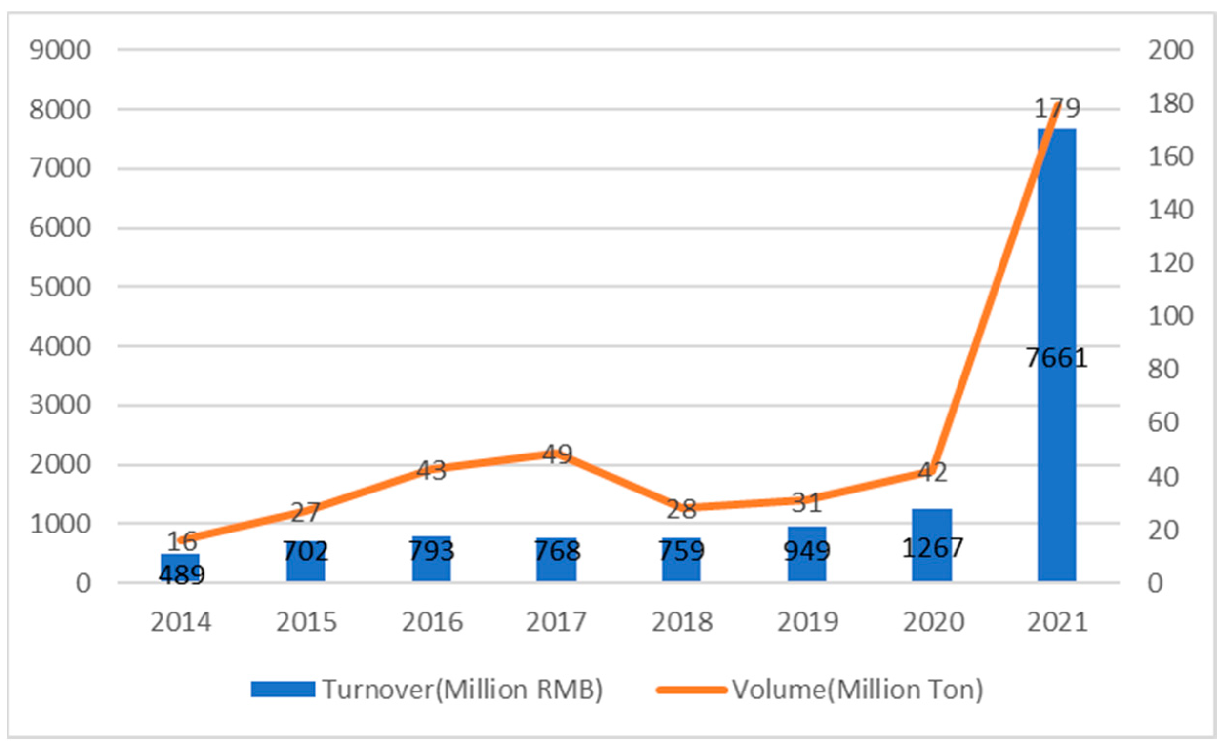
At present, instead of carbon taxes, China mainly relies on ETS to mitigate effects of carbon emissions. Since 2013, China has promulgated ETS pilots in eight provinces or cities, including Beijing, Shanghai, Tianjin, Shenzhen, Chongqing, Guangdong, Hubei, and Fujian [25]. China Carbon Emission Trade Exchange (CCETE), the carbon emissions trading system covering all regions of China’s mainland, was launched on 19 December 2017, and put into operation officially on 16 July 2021. It can be seen from Figure 1 that the scale of carbon emissions trading has increased significantly after the official operation of CCETE.
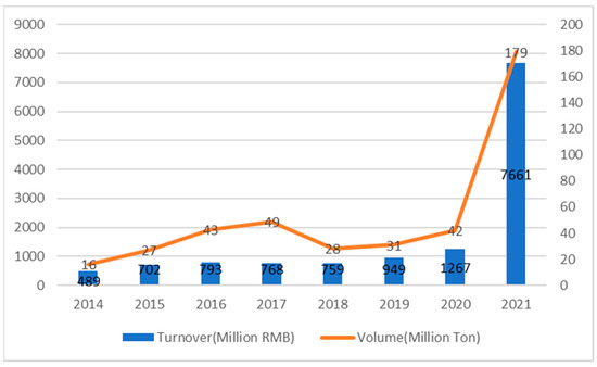
Figure 1.
The carbon emissions trading data of China. Source: Huajing Database. http://www.huaon.com (accessed on 20 May 2020).
However, an ETS cannot solve all the problems of carbon emissions of China, so other emission reduction policy tools should be employed, such as a carbon tax [26]. Carbon taxes can complement the ETS, and using a carbon tax as a supplement is a good mitigation strategy to release Gross Domestic Product (GDP) loss in China [27]. In addition, ETS still has many inefficiencies, so economists prefer to use carbon taxes as policy tools to reduce greenhouse gas (GHG) emissions [28]. In summary, it is necessary to consider carbon taxes as policy options for China in the long run. In view of the impact of carbon taxes on the distribution and the Chinese government’s efforts to narrow the poverty gap and achieve common prosperity in recent years, it is of great practical significance to research carbon taxes and the distribution issue in China.
Compared with carbon emissions trading, carbon taxation can offset the negative externalities more directly and effectively and leads to better predictability in business, easier cost accounting, and lower administrative costs [29]. Therefore, many countries have adopted carbon taxation as one of the most effective policy measures to reduce carbon emissions, such as Finland (1990), Poland (1990), Sweden (1991), Norway (1991), Denmark (1992), Slovenia (1996), Estonia (2000), Latvia (2004), Switzerland (2008), Liechtenstein (2008), Ireland (2010), Iceland (2010), Ukraine (2011), Japan (2012), France (2014), Mexico (2014), Spain (2014), Portugal (2015), Colombia (2017), Chile (2017), Argentina (2018), Singapore (2019), and South Africa (2019) [30].
3. Data and Methods
3.1. Data
The input–output data used in this paper are from the 2012 Input–Output Accounts (IOA) of China compiled by the National Bureau of Statistics of China, which contains 139 departments. The total consumption data of crude oil and natural gas are from the 2012 Energy Balance Accounts (EBA) of China, and the consumption data of crude oil and natural gas by various industrial sectors are from the 2012 Energy Consumption Accounts (ECA) of China. The income and consumption data of urban and rural households are from the China Statistical Yearbook of 2012.
3.2. The Base of a Carbon Tax Payment
In this paper, the primary energy sectors, the upstream production sectors, is set as the tax base, meaning the government levies a carton tax on primary energy input of various industries. The energy sectors listed in the 2012 IOA of China include coal mining and processing, crude oil and natural gas extraction, petroleum, coking, and nuclear fuel processing, the production and supply of electric power and other heat sources, as well as the production and supply of fuel gas. The first two are primary fossil energy sectors, and they are upstream sectors of the other energy sectors. The carbon content of the other energy and production sectors entirely comes from them, and therefore a carbon tax on the output of the primary energy sector can cover the carbon emissions of the whole economic system. If the output of all energy sectors or all production sectors is taxed, there would be double taxation.
3.3. Input–Output Price Model
A carbon tax imposed on energy sectors will inevitably increase input costs for other downstream enterprises, which will, in turn, lead to higher output prices in all sectors through industrial effects. Employing the method used by Metcalf [5], we use the input–output price model to analyze the price interactions between sectors. Similarly to the horizontal equilibrium in quantity model, the vertical balance of the IOA can be achieved in the price model.
where denotes the output value of sector j, is the price of product i, is the input amount of product i to sector j, and is the added value of sector j. Dividing two sides of the equation by , the following equations can be obtained:
. Setting all to be “1”, the equations can be expressed in the following matrixes:
Equation (3) can be denoted as , where is the transpose matrix of the direct consumption coefficient matrix , and is the value-added rate vector for each sector. We can solve the price vector as follows, and P will be a vector of ones:
If a tax is imposed on the system, the elements of vector P will be greater than 1, representing the ratio of the new price to the original one, and the greater-than-1 part is the price increase resulting from the tax. When setting as the ad valorem tax levied on the intermediate products provided by sector j during the production process, Equation (1) will be transformed into:
The set of equations can be manipulated, and then we obtain:
The element of B equals . Under the premise that the production technology of all sectors does not change and there is no short-term substitute for primary energy, the price model can be used to examine the impact of taxation on the prices of all sectors in an economy.
3.4. Regrouping the Input–Output Accounts
In the 2012 IOA of China, crude oil and natural gas were combined in one sector. In order to better examine the impact of price changes in various fossil energy sectors on the economy, this study separates the sector into crude oil and natural gas. For this purpose, we had to divide the sector into rows and columns. The most convenient method to divide the usage values in a row is to separate them by the ratio of usage values of two energies. We can achieve usage value by multiplying the energy usage quantity issued in 2012 EBA of China by the market prices of the energy.
Referring to the domestic and foreign market prices and the RMB exchange rate in 2012, the price of crude oil was set at 4949 RMB/ton, and the price of natural gas was 1.9 RMB/cubic meter. The crude oil usage value based on the EBA should be RMB 2,310,139 million, and that of natural gas should be RMB 277,970 million, totaling RMB 2,588,109 million. The domestic production of crude oil and natural gas sectors based on the EBA should be RMB 102,608 and 203,585 million, respectively, totaling RMB 1,230,396 million. Comparing the above total value of usage and domestic production with the corresponding value listed in the IOA (2,603,804 and 1,226,392 million RMB, respectively), it is found that the maximum error does not exceed 0.6%, so the price setting is reasonable to some extent.
However, it is crude to separate the row this way. This is because, by observing the major sectors of inputting crude oil and natural gas in 2012 ECA of China (Table 1 and Table 2), we found that the main sectors using the two energies are not in the same proportion. In fact, the usage structures of the two energies are quite different, and therefore the separation method based on the assumption of the same usage structure is not applicable.

Table 1.
Major sectors of crude oil input.
Table 2.
Major sectors of natural gas input.
Based on the ECA, EBA, and IOA, this study adopts the following separation method: First, to match the two accounts, the 2012 IOA of 139 sectors was condensed into 46 sectors according to the industry catalogue of the ECA. Second, for sectors that feature in both accounts, we multiplied the sectors’ energy usage quantities by setting prices and obtaining the two energies’ usage value ratio per sector. The usage value of “Crude oil and natural gas extraction” in the IOA was then divided by the ratio. There are some contradictory records between the IOA and ECA: Some sectors have no direct energy input in the IOA, but they have usage data in the ECA. Other sectors have energy input records in the IOA, but no data in the ECA. The former situation was ignored, because we want to keep the basic data and the balance of the IOA unchanged. In the latter case, the split had to be based on the ratio of the total usage value of the two energies.
For the vertical separation, since we lack information about the input structure of the two energy sectors via production processes, it can only be assumed that these structures are similar. The separation was based on the ratio of RMB 1,026,808 to 203,585 million, calculated by multiplying the domestic production quantity by the set price.
In this way, the IOA of 139 sectors was condensed to 47 sector accounts. We compared the calculated value based on the EBA, the ECA, and the setting price, with the corresponding value estimated or listed in the IOA after separation. The results are shown in the Table 3 below.
Table 3.
The estimation errors.
3.5. The Carbon Tax Rate
From a collection convenience perspective, the carbon tax rate should be a specific duty rate. In international carbon tax practice, the specific duty is basically used. Denmark began to levy a carbon tax in 1992, and the tax rate is DKK 100 (Danish kroner)/ton of carbon dioxide (equivalent to USD 14.3/ton of carbon dioxide). In 1995, the Dutch tax rate on carbon dioxide was NLG 5.16 (Dutch guilders)/ton of carbon dioxide (equivalent to USD 2.5/ton of carbon dioxide). The tax rate in Sweden is USD 38.8/ton, and in Finland, it is USD 7/ton of carbon dioxide.
In domestic studies on the impact of a carbon tax in China, the tax rate structure is also designed based on a specific duty. For example, Su et al. [31] proposed a carbon tax scheme of 10 to 40 RMB per ton of carbon dioxide. Wang et al. [32] designed three specific duty schemes in the process of simulating the impact of a carbon tax by CGE. In addition, Fan and Zhang [33] assumed a carbon tax rate of 200 RMB/ton of carbon dioxide in their study of the impact of a carbon tax on the income distribution of urban households in China.
The tax rate in our research is similar to the 75 RMB/ton of carbon dioxide referred to in Wang et al. [32]. In fact, the tax rate has little effect on the conclusion of this study, as the tax rate only increases or reduces the absolute value of consumption expenditure after taxation—it has no essential effect on the trend of progressivity or regressivity.
However, the rate should be an ad valorem tax rate in Equation (5) so that we cannot achieve results based on the specific duty rate we adopt. To convert the specific duty rate into an ad valorem tax rate, we use the following formula:
where is the ad valorem tax rate on sector i, is the specific duty rate on carbon dioxide emissions, and denotes the carbon dioxide emissions of sector i (these data can be obtained by multiplying the total consumption of the energy listed in the EBA by the carbon emission coefficient of the energy). is the output value of the energy sector (for a more reasonable estimate of ad valorem tax rates, the output value is actually the total usage value of the energy sector, and equals the domestic production of the sector plus its net import value). Since the ad valorem tax rates of the same energy should be equal when they are applied to any downstream sector j, we have in Equation (5).
3.6. The Impacts on Consumption Expenditure
In the Consumption Expenditure Accounts (CEA) of urban and rural households with different income groups issued by the National Bureau of Statistics, consumer goods are classified into eight categories that do not match the IOA sector catalogue. The price changes of 47 sectors calculated by the input–output price model should therefore be converted into price changes of eight categories through a transformation matrix:
where is the price vector of the eight categories of consumer goods after taxation, denotes the transposed matrix of the price transformation matrix , and is the price vector of the 47 sectors after taxation. In , the corresponding relationship of sectors between the IOA and CEA refers to the classification in Classification of Consumer Expenditure for Residents (2013), published by the National Bureau of Statistics and the relevant research of Fan and Zhang (2013) [33]. The value in represents the proportion of the final household consumption of goods i in the total consumption of goods category j, and .
Based on the price changes in eight categories of consumer goods, we can calculate the per capita consumption expenditure of different income groups after taxation by formula Equation (9):
where is a vector that reflects the total expenditure per capita of different income groups after taxation and n is the number of income groups. The National Bureau of Statistics divides urban households into seven income groups and rural households into five income groups. is the per capita consumption composition matrix of urban and rural households of different income groups in 2012. Taking rural households as an example, the structure is shown as Table 4:
Table 4.
The composition of rural households’ per capita consumption expenditure.
3.7. The Impacts on Distribution Structure
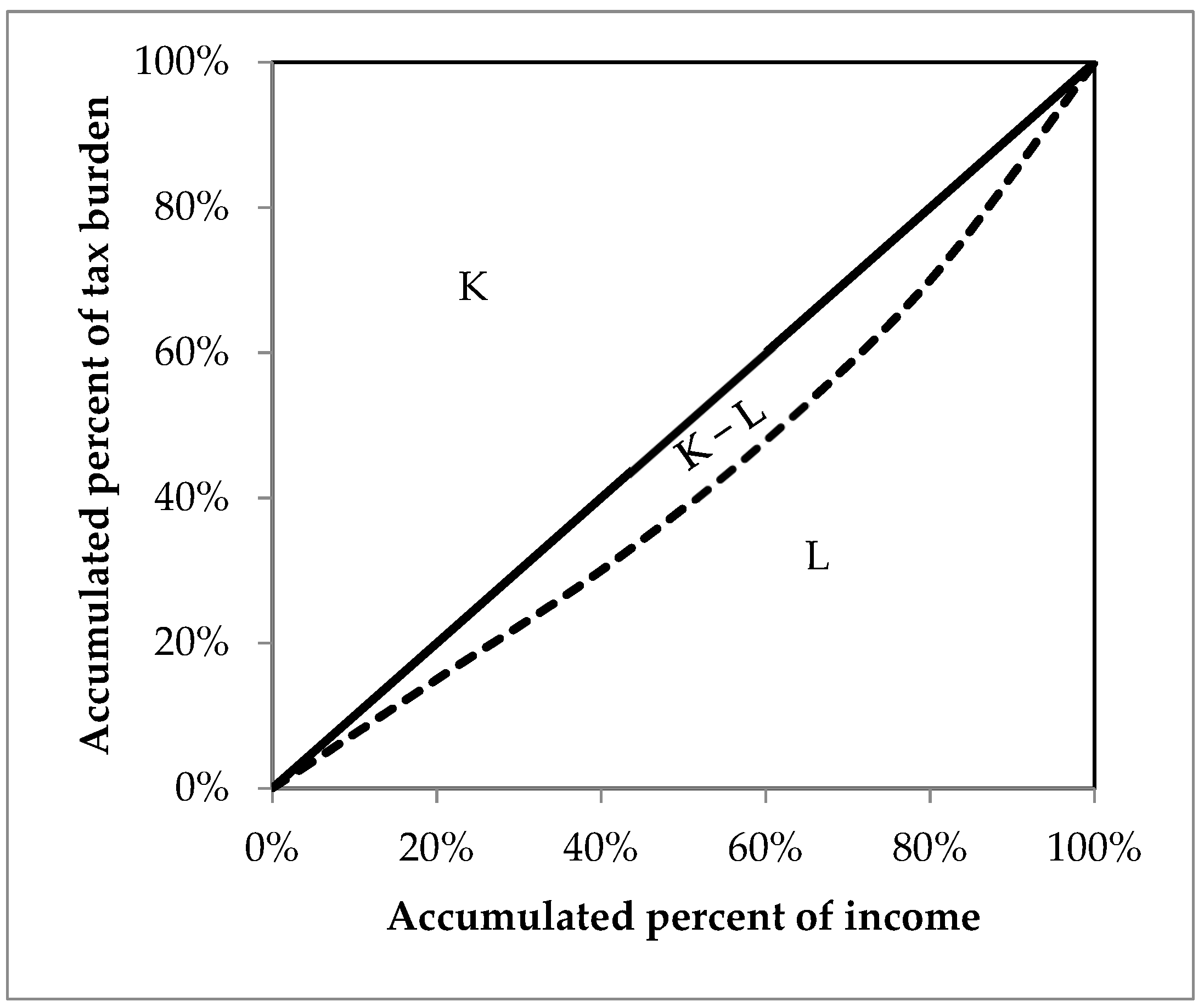
The impact of a carbon tax on consumption expenditure cannot reflect its distribution effects. To examine the impact, the tax burden must be linked to income. The Suits index, proposed by Suits [34], is widely used in the test of tax progressivity and regressivity. The progressive and regressive nature can tell us how a specific tax affects the distribution structure. If the tax is progressive, it will help to improve the distribution structure and narrow the gap between rich and poor. If the tax is regressive, it will lead to the deterioration of the distribution structure and will widen the gap between rich and poor. The Suits index can be illustrated by the concentration curve in Figure 2. The horizontal axis is the cumulative proportion of income, and the accumulated percentage curve of the tax burden is plotted vertically, corresponding to the accumulated percentage of income on the horizontal axis. The Suits index equals ((K − L))/K, where K is the area of the triangle surrounded by the 45-degree line and the horizontal axis, and L is the area surrounded by the curve and the horizontal axis. When K is greater than L, the index is positive and the tax is progressive; when K is smaller than L, the index is negative and the tax is regressive.
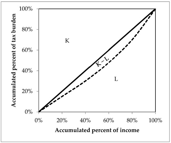
Figure 2.
Concentration curve.
The data obtained in most studies are discrete, so that the area cannot be calculated by integral. Suits (1977) [27] proposed the following formula to approximate the Suits index:
where S denotes the Suits index, is the cumulative percentage point of income, is the cumulative percentage point of tax burden corresponding to the income, and n is the number of income groups.
4. Results and Discussions
4.1. The Impacts on Consumption Prices
The table below shows the prices of the 47 sectors after tax. Since the prices are all “1” before tax, the higher-than-one part reflects the increase after tax.
After transforming, the price changes in eight categories of goods are as Table 5 and Table 6. In IOA, the final household consumption is divided into urban and rural regions. The urban and rural consumption price changes can therefore be calculated separately.
Table 5.
The prices of 47 sectors after tax.
Table 6.
The prices of eight categories of goods after taxation.
According to the results, the changes in the categories for food, clothing, property, household facilities, and articles, as well as education, culture, and entertainment are less in urban areas than in rural areas, while the other three categories are the opposite. Overall, the prices of food, healthcare and medical services, education, culture, and entertainment, as well as miscellaneous goods and services increased slightly (all less than 1%). Property-related cost increases (including gas, water, and electricity, but excluding household purchases) were more than 7.5% in urban as well as rural areas. Prices in the other three categories increased between 1.2% and 1.9%.
4.2. The Impact on Consumption Expenditure
The impact of a carbon tax on the total per capita consumption expenditure of urban and rural households is shown in the Table 7 and Table 8 below.
Table 7.
Total expenditure changes of rural income groups.
Table 8.
Total expenditure changes of urban income groups.
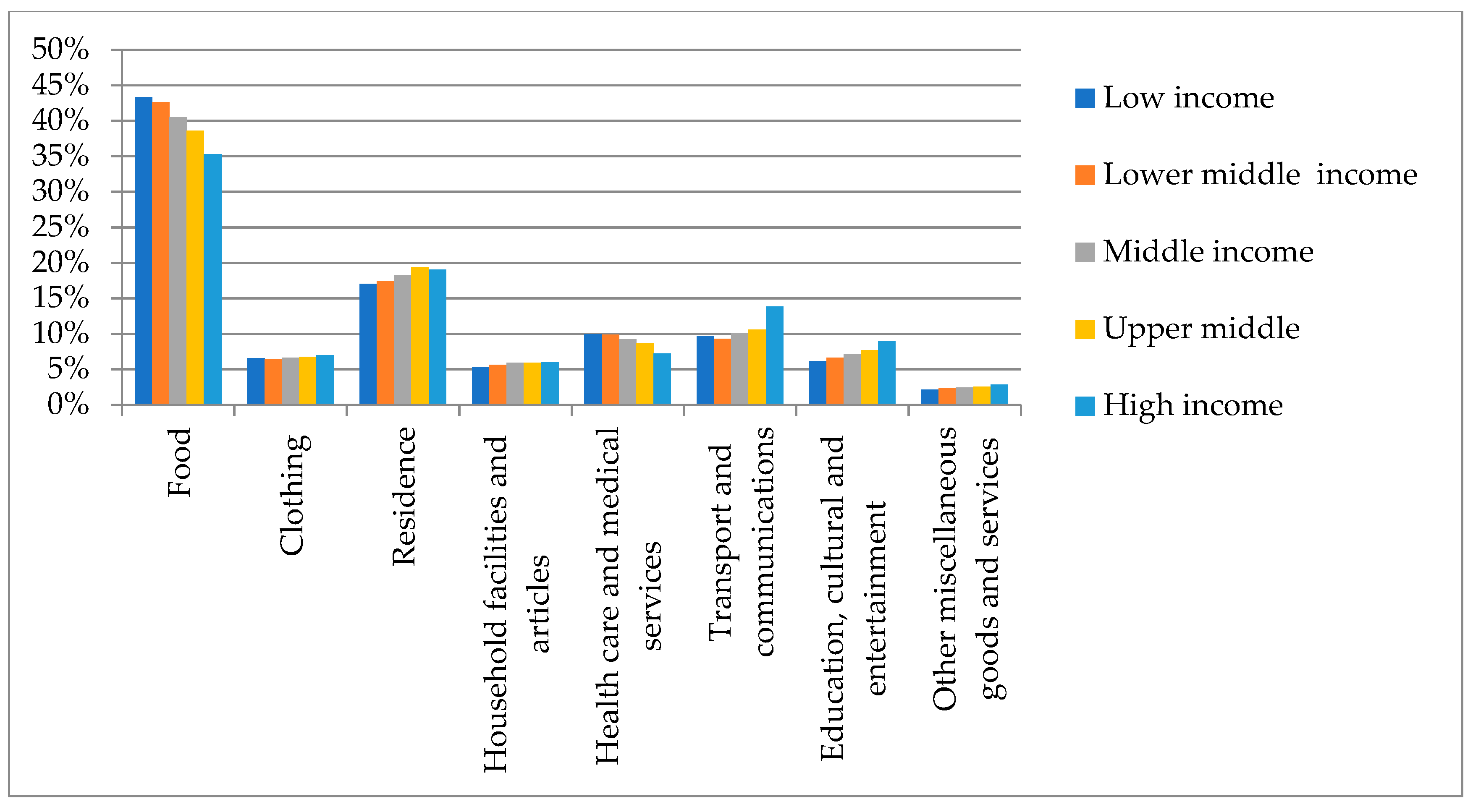
The increased expenditure can be understood as the carbon tax burden transferred from upstream sectors to end-users via the input–output effect. The results indicate that with respect to rural areas, the expenditure increases will affect higher-income groups the most. By observing the expenditure increase in a certain category of goods in relation to the total expenditure of each income group in rural areas, we found that the percentage of food and medical expenditure is negatively correlated with income, while other categories of goods are positively correlated. This means that if rural household income is lower, the percentage of food and medical expenditure is higher. According to Table 6, the price increases of the two groups are relatively low. The price of major consumer goods has therefore increased slightly for low-income rural households, whereas for high-income rural households it has increased considerably. If consumption expenditure is taken as the benchmark, higher-income households’ expenditure increases at a higher rate (Figure 3).
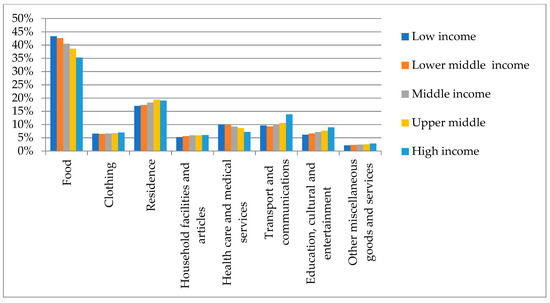
Figure 3.
The expenditure pattern of rural income groups.
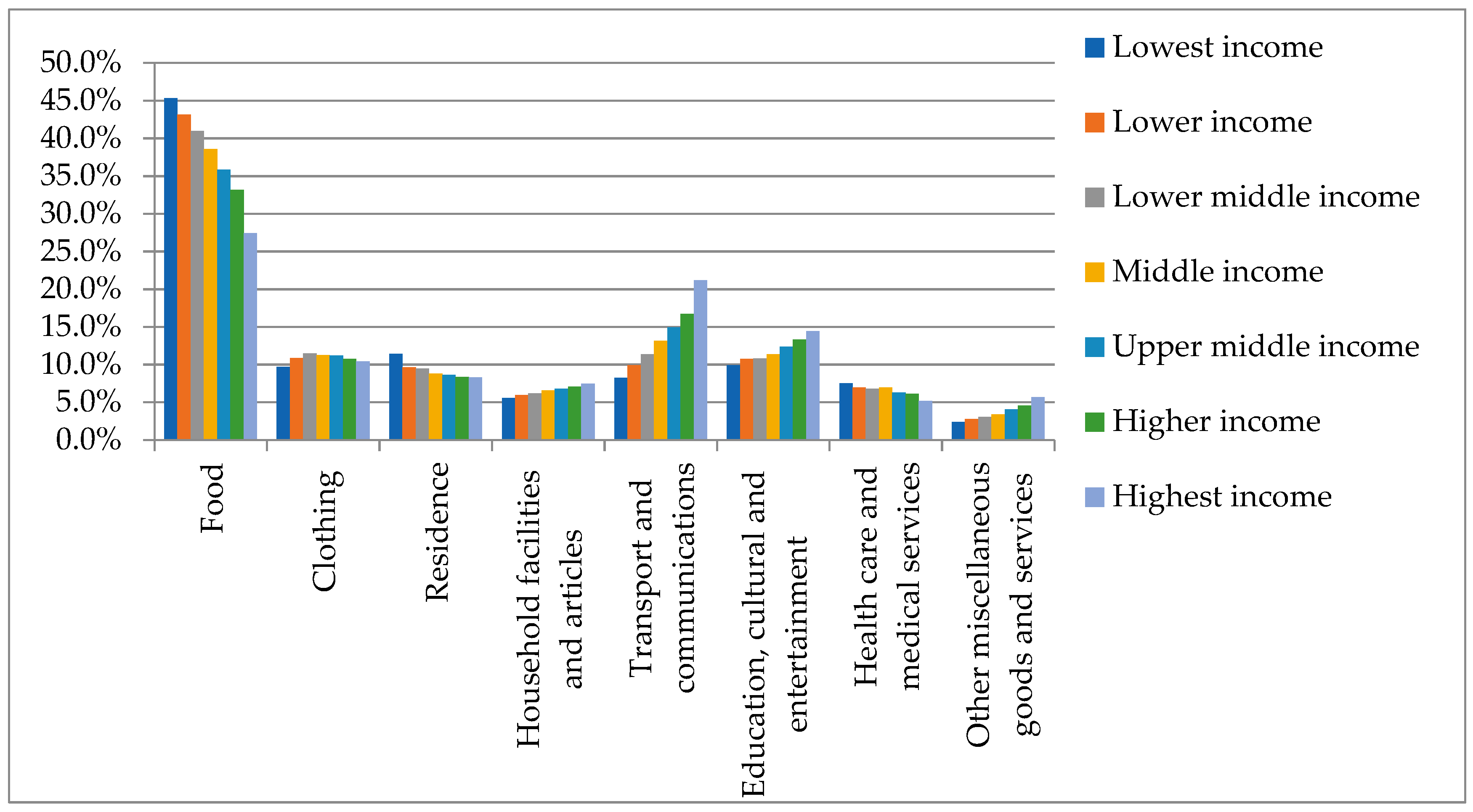
The situation in cities is more complicated. The increase rate of middle-income households is the lowest (1.6595%). Then, the rate changes gradually increase in both directions. The only exception is the lower-income group, whose increase rate is lower than that of lower-middle-income group. In addition, the expenditure growth of the highest-income families is smaller than that of the lowest-income group. We also compared the percentages of all kinds of consumption expenditure in relation to the total expenditure of urban households and found that the percentage of property-related expenditure shows a reversed change with income in urban areas. Because carbon tax increases property-related expenses by 7.6747%, which is the largest increase in all kinds of expenditure, it leads to a higher increase in the per capita household expenditure of lower-income families in urban areas (Figure 4).

Figure 4.
The expenditure pattern of urban income groups.
Overall, the increased expense rate is higher for rural consumers than in urban areas. The range in urban areas is from 1.6595% to 1.7695%, while it is between 2.1967% and 2.3826% in rural areas, which can be explained by the high percentage (15% to 20%) of property-related expenses in rural areas. In urban areas, this percentage is less than 10%, except for the lowest-income group, for whom it is slightly higher than 10%. As mentioned above, the price increase in the property category is the highest. This leads to a greater proportional impact on rural households than on urban ones.
4.3. The Impact on Distribution Structure
Although the situation in urban areas is not clear, it seems that in rural areas the expenditure burden brought about by a carbon tax will be the most severe on the higher-income group. This is progressive, but we must consider income and expenditure together with the distributional analysis of taxation. In this study, we analyze the percentage of expenditure growth in relation to income, which makes it easier to observe the impact of tax on income distribution among different income groups and areas. From Table 9 and Table 10, it is clear that if a group has a lower income, the impact will be more severe, whether the group is in a rural or urban area. That is a significant manifestation of a regressive tax.
Table 9.
The expenditure growth in income in rural areas.
Table 10.
The expenditure growth in income of urban areas.
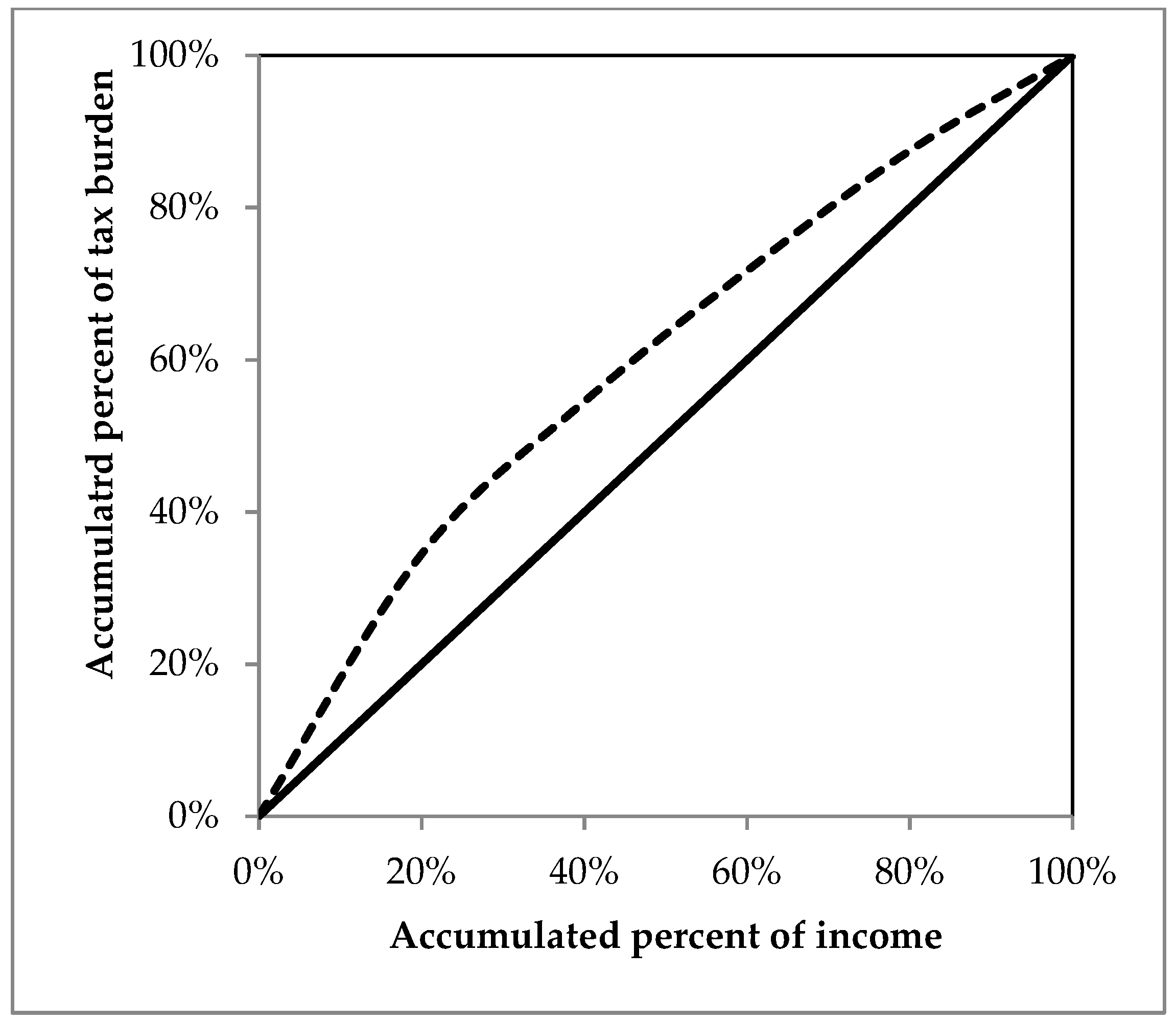
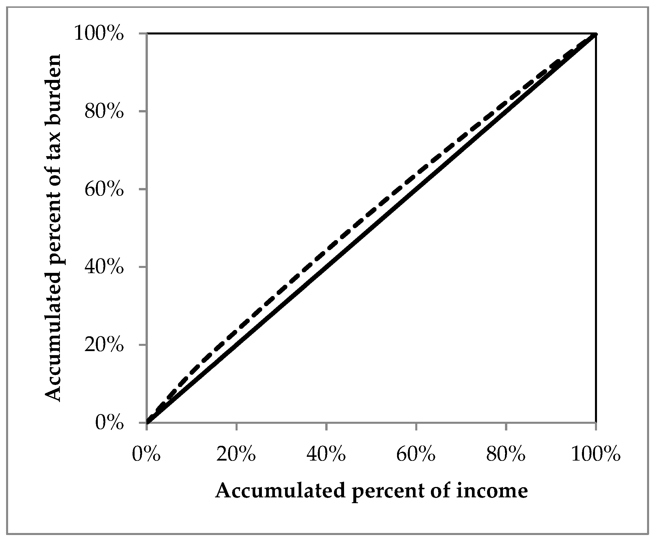
In order to portray the regressive nature of the tax accurately, we employ the Suits index. The concentration curves of the Suits index in Figure 5 and Figure 6 show that a carbon tax, regardless of whether it affects rural or urban households, is indeed regressive, and that the regressive degree in rural areas is much higher than in urban areas. The approximate index values of rural and urban areas are −0.1928 and −0.0588.

Figure 5.
Concentration curves of rural areas.
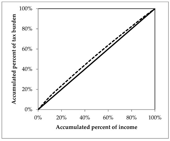
Figure 6.
Concentration curves of urban areas.
4.4. Discussions
The results show that the prices of goods in eight categories increased in varying degrees, the highest being the property category. Due to the high ratio of property-related expenses, the increased expenditure in rural areas is generally higher than in urban areas. We noticed that this mostly affects the higher-income groups in rural areas. In our opinion, this does not mean that a carbon tax will be constructive in China’s rural areas.
Furthermore, by estimating the increased revenue expenditure and the Suits index, we found that a carbon tax will not be constructive in either urban or rural areas, especially in rural areas. Relative to income, the cost impact on lower-income groups will be greater than the effect on higher-income groups. Similarly, higher prices will affect rural households more than urban ones. The consumption structure of Chinese households will influence the impact of a carbon tax on income distribution.
The distribution structure itself will also affect the consequences of a carbon tax. Based on our data, the gap between increased expenditure and income is smaller in rural areas than in urban ones, which results in higher regressivity in rural areas. It is recommended that governments adjust the consumption structure or improve the distribution structure in order to change the impact direction of carbon tax on distribution.
5. Conclusions
The input–output quantity model may not correctly estimate the growth in consumption expenditure after taxation without the assumption of linear tax payment. However, the price model can better reflect the price-linked changes among sectors so that it can simulate the growth in households’ expenditure more accurately.
An important theory on environmental tax is the “double-dividend hypothesis”, according to which governments can diminish the regressive effect of carbon tax by tax revenue redistribution. The design of the tax-recycling policy should be focused on adjusting consumption structures and narrowing the income gap. Some policy options could be subsidies for target groups and sectors, payroll tax reduction, or transfer payment policy.
From our results, it is recommended that the government should pay attention to the different impacts of a carbon tax on rural and urban areas. Except for the high-income group in rural areas, all other income groups in these areas bear a higher tax burden than urban groups. If the government does not apply different policies in urban and rural areas respectively, the income gap between the areas will widen. This is not conducive to transforming a dualistic society to a modern one.
According to these conclusions and discussions, it is strongly suggested that the Chinese government should adopt tax-recycling measures aimed at narrowing the gap between different income groups in urban and rural areas when a carbon tax is levied. It would be beneficial to establishing a harmonious society.
Author Contributions
Conceptualization, S.-M.L.; Formal analysis, Y.-Y.G.; Methodology, J.-X.L.; Validation, J.-X.L.; Writing—original draft, Y.-Y.G.; Writing—review & editing, J.-X.L. and S.-M.L. All authors have read and agreed to the published version of the manuscript.
Funding
This research received no external funding.
Institutional Review Board Statement
Not applicable.
Informed Consent Statement
Not applicable.
Data Availability Statement
Data available on request.
Conflicts of Interest
The authors declare no conflict of interest. This research did not receive any specific grant from funding agencies in the public, commercial, or not-for-profit sectors.
References
- Diamond, J.; Zodrow, G. Carbon taxes: Macroeconomic and distributional effects. In Prospects for Economic Growth in the United States; Cambridge University Press: Cambridge, UK, 2021; pp. 195–244. [Google Scholar]
- Jiang, Z.J.; Shao, S. Distributional effects of a carbon tax on Chinese households: A case of Shanghai. Energy Policy 2014, 73, 269–277. [Google Scholar] [CrossRef]
- Cramton, P.; Mackay, D.J.; Ockenfels, A.; Stoft, S. Global Carbon Pricing: The Path to Climate Cooperation; The MIT Press: Cambridge, MA, USA, 2017. [Google Scholar]
- Poterba, J.M. Is the gasoline tax regressive? Tax Policy Econ. 1991, 5, 145–164. [Google Scholar] [CrossRef] [Green Version]
- Metcalf, G.E. A distributional analysis of green tax reforms. Natl. Tax J. 1999, 52, 655–682. [Google Scholar] [CrossRef]
- Jacobsen, H.K.; Birr-Pedersen, K.; Wier, M. Distributional implications of environmental taxation in Denmark. Fisc. Stud. 2003, 24, 477–499. [Google Scholar] [CrossRef] [Green Version]
- Kerkhof, A.C.; Moll, H.C.; Drissen, E.; Wilting, H.C. Taxation of multiple greenhouse gases and the effects on income distribution: A case study of the Netherlands. Ecol. Econ. 2008, 67, 318–326. [Google Scholar] [CrossRef]
- Shammin, M.R.; Bullard, C.W. Impact of cap-and-trade policies for reducing greenhouse gas emissions on U.S. Households. Ecol. Econ. 2009, 68, 2432–2438. [Google Scholar] [CrossRef]
- Bureau, B. Distributional effects of a carbon tax on car fuels in France. Energy Econ. 2011, 33, 121–130. [Google Scholar] [CrossRef] [Green Version]
- Brenner, M.D.; Riddle, M.; Boyce, J.K. A Chinese sky trust? Distributional impacts of carbon charges and revenue recycling in China. Energy Policy 2007, 35, 1771–1784. [Google Scholar] [CrossRef]
- Symons, E.J.; Speck, S.; Proops, J.L.R. The Effects of Pollution and Energy Taxes across the European Income Distribution; Department of Economics, Keele University: Keele, UK, 2000. [Google Scholar]
- Tiezzi, S. The welfare effects and the distributive impact of carbon taxation on Italian households. Energy Policy 2005, 33, 1597–1612. [Google Scholar] [CrossRef]
- Yusuf, A.A.; Resosudarmo, B. On the Distributional Effect of Carbon Tax in Developing Countries: The Case of Indonesia; Department of Economics, Padjadjaran University: Bandung, Indonesia, 2007. [Google Scholar]
- Dissou, Y.; Siddiqui, M.S. Can carbon taxes be progressive? Energy Econ. 2014, 42, 88–100. [Google Scholar] [CrossRef]
- Malerba, D.; Gaentzsch, A.; Ward, H. Mitigating poverty: The patterns of multiple carbon tax and recycling regimes for Peru. Energy Policy 2021, 149, 111961. [Google Scholar] [CrossRef]
- Hassett, K.A.; Mathur, A.; Metcalf, G.E. The incidence of a U.S. carbon tax: A lifetime and regional analysis. Energy J. 2009, 30, 157–179. [Google Scholar] [CrossRef] [Green Version]
- Rausch, S.; Metcalf, G.E.; Reilly, J.M. Distributional impacts of carbon pricing: A general equilibrium approach with micro-data for households. Energy Econ. 2011, 33, 20–33. [Google Scholar] [CrossRef] [Green Version]
- Zhang, M.; Zhang, J.; Tan, Z.; Wang, D. Analysis on effects of carbon taxation on economic development, energy consumption and income distribution. Technol. Econ. 2009, 28, 48–95. (In Chinese) [Google Scholar]
- Liang, Q.M.; Wei, Y.M. Distributional impacts of taxing carbon in China: Results from the CEEPA model. Appl. Energy 2012, 92, 545–551. [Google Scholar] [CrossRef]
- Zhang, H.X.; Hewings, G.; Zheng, X.Y. The effects of carbon taxation in China: An analysis based on energy input-output model in hybrid units. Energy Policy 2019, 128, 223–234. [Google Scholar] [CrossRef]
- Wang, Q.; Hubacek, K.; Feng, K.S.; Guo, L.; Zhang, K.; Xue, J.J.; Liang, Q.M. Distributional impact of carbon pricing in Chinese provinces. Energy Econ. 2019, 81, 327–340. [Google Scholar] [CrossRef] [Green Version]
- Sun, W.; Ueta, K. The distributional effects of a China carbon tax: A rural-urban assessment. Kyoto Econ. Rev. 2011, 80, 188–206. [Google Scholar]
- Metcalf, G.E. Cost Containment in Climate Change Policy: Alternative Approaches to Mitigating Price Volatility; NBER Working Paper Series, Working Paper 15125; National Bureau of Economic Research: Cambridge, MA, USA, 2009. [Google Scholar]
- Wen, T.J.; Lu, H. The connotation conversion and problem domain of three rural issues and three governance issues in the new era. J. Xi‘Inst. Financ. Econ. 2019, 4, 5–16. (In Chinese) [Google Scholar]
- Yan, Y.; Zhang, X.; Zhang, J.; Li, K. Emissions trading system (ETS) implementation and its collaborative governance effects on air pollution: The China story. Energy 2020, 138, 111282. [Google Scholar] [CrossRef]
- Runst, P.; Thonipara, A. Dosis facit effectum why the size of the carbon tax matters: Evidence from the Swedish residential sector. Energy Econ. 2020, 91, 104898. [Google Scholar] [CrossRef]
- Lin, B.Q.; Jia, Z.J. Can carbon tax complement emission trading scheme? The impact of carbon tax on economy, energy and environment in China. Clim. Change Econ. 2020, 11, 29. [Google Scholar] [CrossRef]
- Metcalf, G.E. Carbon Taxes in Theory and Practice. Resour. Econ. 2021, 13, 245–265. [Google Scholar] [CrossRef]
- Baranzini, A.; Goldemberg, J.; Speck, S. A future for carbon taxes. Ecol. Econ. 2000, 32, 395–412. [Google Scholar] [CrossRef]
- World Bank Group. State and Trends of Carbon Pricing. 2019. Available online: https://openknowledge.worldbank.org/handle/10986/31755 (accessed on 20 May 2022).
- Su, M.; Fu, Z.H.; Xu, W.; Wang, Z.G.; Li, X.; Liang, Q. The research of levying carbon tax in China. Rev. Econ. Res. 2009, 72, 2–16. (In Chinese) [Google Scholar]
- Wang, J.N.; Yan, G.; Jiang, K.J.; Liu, L.C.; Yang, J.T.; Ge, C.Z. The Study on China’s carbon tax policy to mitigate climate change. China Environ. Sci. 2009, 29, 101–105. (In Chinese) [Google Scholar]
- Fan, Y.; Zhang, H. Income distribution impacts of carbon tax on Chinese urban residents and the design of carbon subsidy scheme. Econ. Theory Bus. Manag. 2013, 7, 81–91. (In Chinese) [Google Scholar]
- Suits, D.B. Measurement of tax progressivity. Am. Econ. Rev. 1977, 67, 747–752. [Google Scholar]
Publisher’s Note: MDPI stays neutral with regard to jurisdictional claims in published maps and institutional affiliations. |
© 2022 by the authors. Licensee MDPI, Basel, Switzerland. This article is an open access article distributed under the terms and conditions of the Creative Commons Attribution (CC BY) license (https://creativecommons.org/licenses/by/4.0/).