Abstract
Wave features and propagation characteristics during typhoons are the key factors to study the dynamic response of ocean engineering and coastal disaster prevention and mitigation under extreme climate. Based on the Longuet-Higgins theory, the method of the field spectrum during the typhoon was used to compute the typhoon waves. And the directional spectrum, the formulas of wave surface, the velocity of water particles, and the acceleration of water particles were investigated. The results showed that the interpolated field wave spectrum combined with the SWOP direction spectrum could accurately simulate the three-dimensional typhoon waves. The significant wave height and the average period of the simulated wave surface at fixed point were statistically evaluated by the upward zero-crossing method, and the relative errors were ± 5% and ± 15%, respectively. The typhoon wave surface computed by a dual peak spectrum had small periodic waves, and the velocity and acceleration of water particles differed considerably from the JONSWAP spectrum. Finally, a fastened slender cylinder was simulated under action of the typhoon waves, which proved the applicability of the computation method. This study aims at providing a basis for the simulation of the dynamic response of marine structures under the typhoon waves action.
1. Introduction
Marine disasters occur frequently in China. Most marine disasters are caused by typhoon waves [1], and ocean waves are complex random waves. The method of wave spectrum, which is used to describe wave features by random process, has become the research mainstream. The widely used wave spectrum includes frequency and directional spectrum. The frequency spectrum consists mainly of P-M spectrum, TMA spectrum, JONSWAP spectrum, and Wallops spectrum [2]. And the directional spectrum mainly include the directional distribution function of Longuet-Higgins, the directional distribution function of Donelan, and the directional distribution function of SWOP spectrum [3]. Moving typhoons can cause significant variations in wave features, including significant wave height, directional spectrum, and wave propagation [4]. Many scholars have focused on studying the relationship between wave features and typhoon characteristic (typhoon path, propagation velocity, and duration), in recent years [5,6,7,8]. Many studies have shown that the spectrum structure of typhoon waves are quite complicated. Thus, a large number of filed typhoon data showed that typhoons were usually mixed waves with coexistence of wind waves and swells. Except for commonly single peak spectrum, most field spectrum were dual peak or multi peak [9,10,11,12,13]. The dual peak field spectrum was used to simulate the wave features of typhoon, which can accurately reflect the actual sea conditions and provide a reference for the prevention of ocean engineering.
A method, which employed the two single-peak spectra to describe dual peak wave spectrum, was first proposed by Strekalov et al. [14]. Then, a formula of dual peak wave spectrum with six parameters based on the field spectrum data of the North Atlantic was developed by Ochi & Hubble [15]. The dual peak wave spectrum includes low-frequency and high-frequency parts, and each part contains three parameters, namely, effective wave height, spectral peak frequency and shape parameters. Later, a dual peak wave spectrum with four parameters was introduced by Guedeos [16], and he combined the two JONSWAP spectra to fit 1000 field spectra in the North Atlantic and 6000 spectra in the North Sea. In recent years, many scholars have improved the parameters of classical dual peak wave spectrum through a large amount of field spectrum data, and they verified that the Ochi-Hubble spectrum and the JONSWAP spectrum could well describe the characteristics of the dual peak spectrum of typhoon wave [17,18,19]. However, these formulas were just fitted by the field spectrum in a specific sea, and they only consider the distribution of wave energy in the frequency range. Therefore, there were great limitations in describing the distribution under different wave directions.
In actual sea conditions, typhoon waves are often mixed waves, which composed of the wind wave and swell of different frequencies and directions. The formula of wave frequency spectrum can only describe variation of the wave surface at a fixed point with time. The actual wave surface is three-dimensional, and its energy is not only distributed in a certain frequency range, but also in a wide range of directions [2]. The introduction of directional spectrum S (f, θ) can more accurately describe the characteristics of ocean waves [20,21,22,23]. The formula is as follows:
where S(f) denotes non-directional spectrum, and S(f, θ) directional spreading function. SAR image technology was used by Sun et al. [24] to extract the direction spectrum of ocean waves. The three-dimensional spectrum method was first used by Panahi to simulate the coastal waters of Oman Bay [17]. The result showed that the method could more intuitively distinguish wind sea and swell in mixed waves. Currently, the studies of typhoon wave tend to focus on frequency spectrum rather than directional spectrum.
At present, the investigations on typhoons were paid more attention to the duration of the typhoon and the landing path. However, waves generated by the typhoons often pose a serious threat to the safety of marine production activities and marine structures [25,26]. Abdolali et al. [27] developed the WAVEWATCH III wave model to Large-scale hurricane modeling using domain decomposition parallelization and implicit scheme. The 3rd generation wave models are really excellent and accurate in simulating typhoons and storm surges. But it is difficult for moored structures to couple with the 3rd generation wave models. Therefore, it is of great significance to study the wave characteristics during the typhoon and to analyze the dynamic response of marine structures. In this paper, we explored the applicability of the widely used Ochi-Hubble and the JONSWAP spectrum in simulating typhoon waves based on the field wave spectrum data in Sanmen Bay. In addition, we proceeded a computation method for the typhoon waves based on the field data. The directional spectrum, and the wave factors were further analyzed. Finally, the motion and force of a moored slender cylinder under the action of the dual peak spectrum of filed typhoon Talim were simulated, which can provide a reference for predicting the influence of Typhoon on the moored structures in the future.
2. Simulation Methods
This section describes the collection and processing method of filed data in Sanmen Bay of China during the Talim typhoon, and the discrete method of directional spectrum of wave is also described.
2.1. Data Collection and Processing Methods
Zhou et al. [28] pointed out that the typhoon Talim (from 20:00 on 9 September to 14:00 on 18 September 2017) approached the Sanmen Bay in the southeast of the East China Sea and then turned to land in Japan as shown in Figure 1. During the action time, it had remarkable influences on the waves in Sanmen Bay Sea area. Large waves caused by typhoons are a key factor in causing damage to offshore and coastal projects. Therefore, this paper selects the typhoon wave spectrum at the time of the maximum wave height (at 11 o’clock on 14 September 2017) as a representative to study the three-dimensional numerical simulation of Typhoon wave characteristics. The water depth is around 7.5 m (geographic position: 29°01.003′ N, 121°42.893′ E), and the wave monitoring point in the SE direction is open to the sea area facing the East China Sea, and there is basically no any islands in this sea area [28], exhibiting a relatively wide waters from the NW direction to the SE direction, and waves observed in multiple directions are well representative. The Storm software provided with the instrument calculates the wave spectrum through the fast Fourier transformation (FFT) method, which are smoothed within the frequency domain with 6 degrees of freedom with a cut-off frequency of 1 Hz and a resolution of 0.01 Hz.
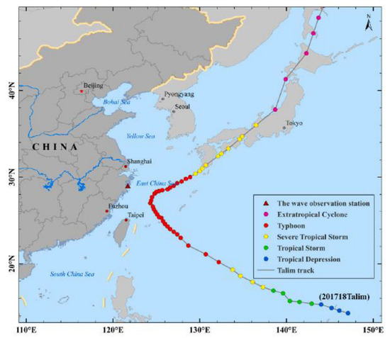
Figure 1.
The trajectory of typhoon Talim. The red star represents Beijing, the capital of China.
The spectrum curve of the maximum wave height is shown in Figure 2. The measured effective wave height H1/3 is 1.58 m, and the spectrum peak period Tp is 13.15 s. The average wave period is 5.96 s. An improved JONSWAP spectrum [29] and a dual peak Ochi-Hubble spectrum [15] were used to fit the field spectrum. Among them, the peak enhancement factor γ of the improved JONSWAP spectrum is 0.95, and can be expressed as follows:
where denotes the average wave period defined by the upward aero-crossing method, and γ represents the peak enhancement factor.
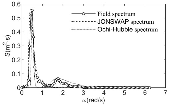
Figure 2.
Wave spectra curve of maximum wave height during the typhoon Talim.
It can be seen from Figure 2 that the spectrum of the typhoon Talim is a mixed wave spectrum dominated by surge. The low-frequency peak of surge part is the maximum peak, and the high-frequency peak of wind wave part is the second peak. The low-frequency peak is much larger than that in the high-frequency peak, and most of the energy of the spectrum is concentrated in the low-frequency part.
The equation of Ochi-Hubble dual peak spectrum [15] can be written follows:
where HS,j, ωp,i and λi for i = 1,2 are significant wave height, angular peak frequency, and spectral shape factor for low and high-frequency parts (i = 1 represents the low frequency spectrum, and i = 2 represents the high frequency spectrum), respectively. Formulation of the six parameters was given. The values of the parameters of the Ochi-Hubble dual peak spectrum (Tp1 and Tp2, the main spectral peak period and the secondary spectral peak period, respectively) are Tp1 = 12.5 s, Tp2 = 3.57 s, Rp1 = 0.65, a1 = 0.61, a2 = 0.94, c1 = 7.32, c2 = 1.0, d1 = 0.0, d2 = 0.102.
As shown in Figure 2, the improved JONSWAP spectrum is a single-peak spectrum, and the field typhoon wave spectrum is a dual peak spectrum, but it is inconsistent with the Ochi-Hubble dual peak spectrum. The field typhoon wave spectrum width of the main spectral peak is closer to the improved JONSWAP spectrum, and the spectral width of the secondary spectral peak is smaller than the calculated value of the dual peak Ochi-Hubble spectrum. Therefore, it is difficult to replace the typhoon wave spectrum by using the statistical spectrum to simulate the three-dimensional wave characteristics of typhoon. In this paper, the interpolation and calculation of wave spectrum will be carried out directly using the field spectrum.
2.2. Discretization Methods of Wave Spectrum
According to the Longuet-Higgins theory [30], the wave is a stationary random process with ergodicity of various states. Therefore, the wave is equivalent to the superposition of an infinite number of simple harmonic cosine waves (linear waves) with unequal amplitude, unequal frequency and random initial phase, as shown in the following Formula (4):
where an and ωn are the amplitude and circular frequency of the constituent waves, respectively, and εn is the initial phase uniformly distributed between 0 and 2π. The target spectrum is a random wave for Sη(ω). ω represents circular frequency, and it needs to be divided into N intervals as Δωi = ωi − ωi-1 = ωH/N. ωH is the circular frequency of the largest constituent wave. Obviously, the circular frequency of the smallest constituent wave is taken as 0. If ωi (randomly selected between ωi and ωi−1) is taken as the representative frequency of the i-th constituent wave, the amplitude of the i-th is shown in Equation (5). Then, by superimposing the N cosine waves of the wave energy in all N intervals, the wave surface line Equation (6) of the ocean wave and the motion Equations (7) and (8) of the two-dimensional water particle can be expressed as:
where Sη represents the ocean wave spectrum, and εi indicates the initial phase of the i-th component wave, which is randomly generated within 0–2π.
where ux and uz are the velocity of the water particle in the x and z directions, respectively; ax and az are the acceleration of the water particle in the x and z directions in turn; (x, z) represents the coordinates of two-dimensional wave field in the vertical direction. d is the water depth, and ki is the wave number of the constituent waves obtained by solving the dispersion equation using the bisectional method.
It follows from Figure 2 that the main circular frequency of the Talim wave spectrum is 0.5 rad/s. When N is a constant, ωH is generally selected as four times the main circular frequency ωp, and the wave simulation accuracy is high. Since the circular frequency is greater than 2.5 rad/s and approaches 0, ωH is selected to be 5 times the main circular frequency, that is, 2.5 rad/s, and the corresponding value of N is also increased to 320. The equal frequency method was used to divide the circular frequency interval as Δωi = 7.81 × 10⁻³. The resolution of the field spectrum in Figure 2 is 0.01 Hz which is 0.063 rad/s, and the field spectrum needs to be interpolated into 320 circular frequency intervals (0–2.5 rad/s). The comparison between the wave after cubic spline interpolation and the original field spectrum is made as shown in Figure 3.
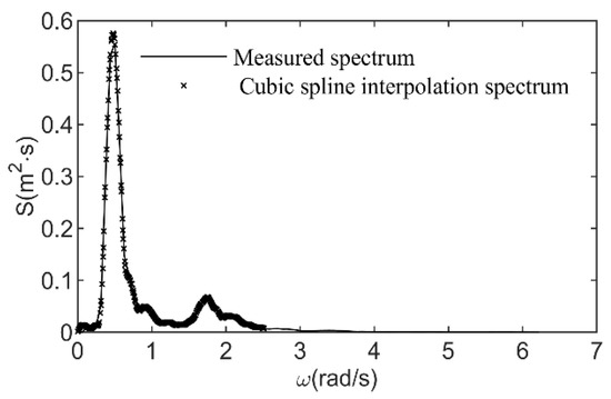
Figure 3.
Comparison between measured spectrum and interpolated spectrum.
2.3. Discretization Methods of Wave Spectrum and Directional Spectrum
The SWOP (Stereo Wave Observation Project) directional spectrum [31] is used as the directional target spectrum for typhoon wave simulation, and the distribution function is shown in Equation (9). In theory, −π < θj < π, but in fact that the energy of the waves is mainly distributed in the range of π/2 on both sides of the main propagation direction, so the number of equally divided angles only on −π/2 < θj < π/2 is M = 30. Assuming that the frequency spectrum and the directional spectrum are mutually independent. The wave spectrum considering the directional spectrum can be obtained by multiplying the two and then superimposing, and the formulas of wave spectrum are expressed in Equation (10) and directional spectrum is shown in Figure 4. With considering the directional spectrum Equation (12), the wave surface and the motion of three-dimensional water particles (Equations (13) to (14)) can be obtained by superimposing the cosine waves in M directions.
where the meanings of mentioned above symbols are the same as the Equations (7) and (8). The velocity and acceleration of water particles, and the subscript j (j represents the wave propagation direction) were added.
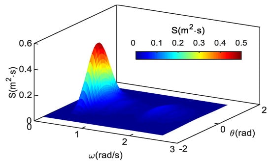
Figure 4.
Three-dimensional directional spectrum.
3. Verification of Wave Features
In order to verify the correctness of the three-dimensional typhoon waves based on the field spectrum, the changes in the wave surface at fixed points x = 0 m and y = 0 m over a period of 840 s were extracted, and the effective wave height and average period of the wave surface were calculated by the upward zero-crossing method. The maximum and minimum points of the random wave surface determined by the method and the duration curve of wave surface at the coordinate (0, 0) are shown in Figure 5. The wave height of a single cycle results from the adjacent maximum point minus the minimum point, and the wave period is the subtraction of two adjacent maximum points (or the subtraction of two adjacent minimum points). Figure 5 shows an enlarged view of the black wireframe part of the above picture. Since ωi and εi are randomly generated in the model, the random wave elements generated at the fixed points are tested by continuous calculation for ten times, as shown in Table 1.
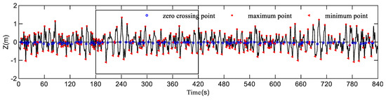
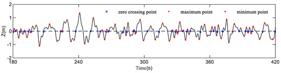
Figure 5.
The duration curve of the wave surface simulation at the fixed point (x = 0 m, y = 0 m) and the wave features determined by upward zero-crossing method.

Table 1.
Ten consecutive typhoon wave simulations and statistical wave features.
According to the filed data, the effective wave height was 1.58 m and the average wave period is 5.96 s at the time of the occurrence of the maximum wave height under the Typhoon Talim action. The error in Table 1 is the relative error between the calculated value and the filed data. It can be seen that the error of the effective wave height is about ±5%, and the error of the average period is about +15%. Zhou et al. [7] pointed out that the measured average period of typhoon waves is Tmean < T01 (mean period of spectral calculation), while Tmean ≈ T01 under deep water conditions. It follows that the water depth affects the calculation of the typhoon wave period, which is also related to the wave theory used. In shallow water, the linear wave theory will increase the value of the average wave period when simulated random waves.
4. Simulation of Typhoon Wave Features
The wave surface, the velocity of water particle, and the acceleration of water particle are the key factors to determine the force and motion of marine floating and suspended structures (ships, buoys, wave energy conversion devices, marine aquaculture equipment, etc.).
4.1. Wave Surface
Based on the field wave spectrum of Typhoon Talim and the numerical calculation of the JONSWAP wave spectrum as show in Figure 2, the duration changes of wave surface of three-dimensional waves is shown in Figure 6. Compared with the JONSWAP wave spectrum, the field wave spectrum is a dual peak spectrum, which has a secondary dominant- frequency in higher frequency. Therefore, a large difference between the wave surface of the typhoon wave and the wave surface simulated by the JONSWAP wave spectrum existed. The specific difference is that there are small-period waves on the water surface of typhoon waves, that is, there are also small-period waves between the peaks and troughs of large-period waves. However, when the incident wave period is close to 1/2 of the natural period of the moored buoy, the buoy will show transverse instability on the free surface and produce resonance, which was proved by Radhakrishnan et al. through flume experiments [32]. The existence of small periodic waves increases the probability of resonance between waves and small-scale floating structures, which not only affects the stability and safety of structures, but also increases the damage of mooring systems.
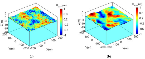
Figure 6.
The 3D typhoon waves surface: (a) the dual peak field spectrum; (b) the single-peak JONSWAP spectrum.
4.2. The Velocity of Water Particle
For small-scale marine structures (structure characteristic length/wavelength <0.2), the Morison equation can be used to calculate the drag force and inertial force of the structure and to obtain the motion response of floating and suspended structures [32]. To simulate the motion response of small-scale structures under the action of typhoon waves, the calculation of the velocity distribution field and acceleration distribution field of the water particles are the key points. The velocity vectors of water particles on the X-Z plane at five water depths (z = 0, −2.5, −5, −10, −15 m) were obtained by using the Equation (13), where y = 0 m, and the positive direction of the X-axis is the main wave propagation direction (with the highest probability density), as shown in Figure 7a. The duration variations in 840 s of the velocity of water particles at coordinate point (x = 0 m, y = 0 m and z = 0 m) is shown in Figure 7b. Since the wave surface line and the velocity of the water particles at the fixed point are superimposed by N linear constituent waves and waves from M different propagation directions, it is difficult to use the peaks or troughs shown in Figure 7a to evaluate the magnitude and direction of the velocity of water particles. The blue line in Figure 7a is the wave surface line, and the velocity vector of water particles also has both small periodic variation and large periodic variation in the X-axis direction. When the wave surface line is changed from being higher than the stilling water surface to being lower than the stilling water surface, the velocity of the water particle is the largest and decreases abruptly along the vertical direction. In Figure 7b, when the wave surface line is lower than the stilling water surface, the velocity of the water particle at the coordinate point (x = 0 m, y = 0 m and z = 0 m) is 0 in each direction. Owing to the special location (the velocity of water particles U in the X direction is equal to velocity of the water particle V in the Y direction), Figure 7b only shows the velocity of water particle U in the X direction and the W in the Z-axis direction. We can see from the Figure 7 that the duration variation in U and W at the fixed point is quite different in the positive and negative directions, and there is no periodic change tendency. There is little difference between the maximum values of U and W, both of which vary between ±1.7 m/s.
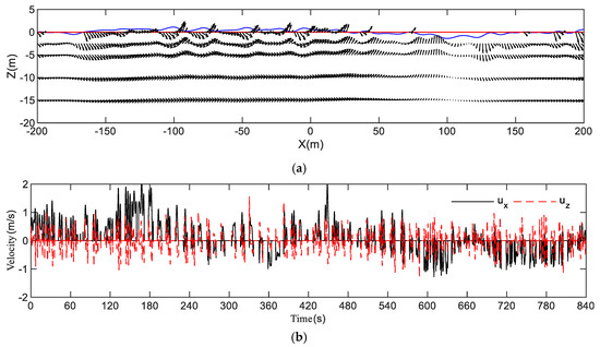
Figure 7.
The velocity of the water particle in the typhoon wave: (a) The velocity vector of the water particle in the x-z plane (y = 0 m); (b) Simulate the duration variations of the water particle velocity in the x-direction (U) and z-direction (W) at the fixed point (x = 0 m, y = 0 m, z = 0 m).
The statistical characteristics of U and W include the maximum value, the average value, the average value of the top 1/3, and the average value of the top 1/10 of the data in Figure 7, which are given in Table 2. The maximum value of data reaches 2.06 m/s, which will lead to terrible damage to offshore structures. It is also found that the forward velocity of U is greater than the reverse velocity. This indicates that there is a drift in the propagation direction of the water particle. On the contrary, the positive and negative directions of W are basically identical.
Table 2.
Statistical wave characteristics of the velocity and of acceleration of water particle.
4.3. The Acceleration of Water Particle
The acceleration vectors of water particles on the X-Z plane at five water depths (z = 0, −2.5, −5, −10, −15 m) were calculated by using the Equation (14), and the results are indicated by Figure 8a.
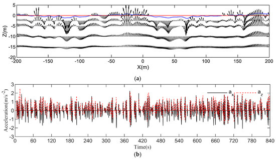
Figure 8.
The acceleration of water particle in the typhoon wave: (a) The acceleration vector of water particle in X-Z plane (y = 0 m); (b) Simulate the duration variations of the acceleration vector of water particle in the x-direction (ax) and z-direction (az) at a fixed point (x = 0 m, y = 0 m, z = 0 m).
Figure 8b shows the 840 s duration variations in the acceleration of water particle at the coordinate point (x = 0 m, y = 0 m and z = 0 m). The acceleration of water particles at the wave peak is upward divergent, but at the wave trough is downward convergent, and it decreases abruptly along the vertical direction. Like the velocity vector of water particle, the acceleration vector of water particle has both small periodic changes and large periodic changes in the x-axis direction. In Figure 8b, when the wave surface line is lower than the stilling water surface, the acceleration of water particle in each direction at the coordinate point are zero (x = 0 m, y = 0 m and z = 0 m).
The statistical characteristics of ax and az are also given in Table 2. The maximum value of az reaches 2.93 m/s2, which will also lead to a large wave inertia force to offshore structures. Different from the velocity of water particle, the positive and negative directions of ax are basically same.
5. Application to a Slender Cylinder Fastened by Mooring Cable
In order to better prove the applicability of the typhoon wave calculated by the above field spectrum, we will add a slender cylinder fastened by mooring cable, and then the motion trajectory of the slender cylinder and the tension of mooring cable were obtained.
5.1. Simulation Method of a Slender Cylinder
- (1)
- Spatial position of structure and wave conditions
This moored structure is mainly composed of a homogeneous and slender cylinder and a mooring cable. One end of the mooring cable is tied to the bottom of the slender cylinder, the other end is in the seabed. The specific physical properties and the geometric parameters of a slender cylinder fastened by mooring cable are listed in Table 3. At the initial time, the top coordinate of the slender cylinder is (0.0, 0.0, 0.0), and the bottom coordinate is (0.0, 0.0, −4.0). The height of the slender cylinder is 4m, and the natural length of the mooring cable is 16m. As a result, the top coordinate of mooring cable is (0.0, 0.0, −4.0), and the bottom coordinates is (0.0, 0.0, −20.0).
Table 3.
The setting parameters of numerical model.
- (2)
- The force and motion of slender cylinder
The slender cylinder was divided into 21 units. According to the Morison equation, the forces acting on the unit of slender cylinder under typhoon waves mainly include drag force and inertia force, as well as the gravity, the buoyancy of seawater and the tension of mooring cable. For the specific calculation methods of the drag force and inertia force of the units of slender cylinder, please refer to Pan et al. [33] and Zhu et al. [34,35]. The drag coefficient and inertia coefficient in x, y z directions are shown in Table 1. In particular, the drag force of the units of slender cylinder was calculated by the relative velocity. The relative velocity is the difference between the velocity of water particle calculated by Equation (7) and the velocity of the units of slender cylinder. The inertial force of the unit of slender cylinder was calculated by the acceleration of water particle in Equation (8). The force of all units of the slender cylinder was accumulated, and the translation acceleration was obtained by dividing the mass of the slender cylinder. It is necessary to calculate the moment of each unit equivalent to the centroid of the slender cylinder, and then divide the moment of inertia to obtain the rotational acceleration, which is reason that the slender cylinder was divided into finite units. The moment of inertia of the slender cylinder is shown in Equation (15).
where Jx, Jy, Jz is the moment of inertia relative to the centroid of the slender cylinder in x, y, z directions. m represents the total mass of the slender cylinder. r is the radius of the slender cylinder, and h is the height. It should be noted that the slender cylinder is sometimes higher than the wave surface in the motion process, so it is necessary to compare each unit of the slender cylinder with the wave surface η calculated by Equation (3). If the z coordinate of the unit of slender cylinder is greater than η, the velocity and acceleration of the water particle are zero, i.e., the wave drag force and inertia force are zero, and the unit is not subject to the buoyancy of the sea water.
- (3)
- The tension and motion of mooring cable
According to the method of Zhu et al. [35], the mooring cable can be divided into 25 lumped mass points. The tension of adjacent points, which mainly includes stiffness force and damping force, was assumed to be a spring. The specific equation is not repeated here. It should be noted that the top and bottom point were not involved in the motion calculation of mooring cable. Without updating the position of the bottom point at each time step, the bottom of mooring cable was fixed on the seabed, while the top point was directly assigned by the position and velocity vector of the bottom unit of the slender cylinder.
5.2. Simulation Results
Under the action of typhoon waves, the motion state of slender cylinder, the maximum tension of mooring cable, and the response frequency of rolling were simulated by the JONSWAP spectrum and field spectrum. In addition, the results were compared and analyzed.
- (1)
- The motion state of slender cylinder and the tension distribution of mooring cable
The motion state of the slender cylinder and the tension distribution of mooring cable at different times under the two spectral conditions are shown in Figure 9, in which the velocity vector of the water particle at different times was marked with arrows in different colors. At the initial time (t = 0 s), the positions of the slender cylinder fastened by mooring cable in different wave model are same, and the mooring cables were not subject to tension. What calls for special attention is that the random numbers produced by random seeds (C++ computer language) in two wave models are same, i.e., the random numbers generated each time are the same. Only in this way can two wave models be compared. In a wave period, the motion state of the slender cylinder only has the translation motion in the y direction and the rolling motion in the X direction. The motion amplitude is between −2 m and +2 m. Due to the secondary peak frequency of the field spectrum, the rolling of slender cylinder in Figure 9b is obviously larger than that in Figure 9a, and the motion state is more complex. As a result, the maximum tension of Figure 9a,b are 5.5 kN and 13.0 kN, respectively. Therefore, the study of dynamic response of moored structures under typhoon waves will not be able to obtain the description of extreme cases only by using JONSWAP spectrum method.
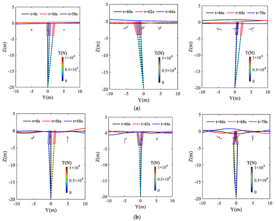
Figure 9.
The motion state of slender cylinder and the tension distribution of mooring cable: (a) The single-peak of JONSWAP spectrum; (b) The dual peak of field spectrum.
- (2)
- The centroid motion of slender cylinder
For the translational motion, the motion trajectory of the lumped masses of the slender cylinder were emphatically analyzed, and the time series of the motion trajectory was converted into a frequency curve by fast Fourier transformation [36]. Furthermore, the response frequency of the translational motion of the slender cylinder was analyzed. Figure 10 and Figure 11 are the time series and converted frequency curves of the centroid motion of the slender cylinder obtained by the JONSWAP and field spectrum. The amplitude and period of the centroid translation of slender cylinder in the Y and Z directions of JONSWAP spectrum and field spectrum are basically identical, i.e., it is not affected by the secondary peak frequency of the field spectrum. In addition, their response frequency and period are also relatively close. On the one hand, their response frequencies are 0.078 Hz and 0.097 Hz, respectively. On the other hand, their corresponding periods are 12.82 s and 10.31 s in turn, and they are close to 12.5 s. In Figure 11b, the motion in Z direction has no peak frequency of response. The reason why this phenomenon happened is that the motion of slender cylinder in the Z direction is mainly affected by the gravity, buoyancy, and the tension of mooring cable.
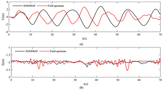
Figure 10.
Time series of the centroid motion of slender cylinder: (a) Y direction; (b) Z direction.
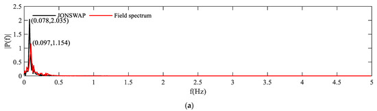
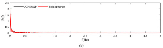
Figure 11.
Frequency curve of centroid motion of slender cylinder: (a) Y direction; (b) Z direction.
- (3)
- The rolling of slender cylinder
Similarly, the angular rotation of slender cylinder around the X axis was transformed into a frequency curve by the fast Fourier transformation method, as shown in Figure 12 and Figure 13. In Figure 12, the amplitude of rotation angle of the JONSWAP spectrum and field spectrum is basically same, but there is a big difference in response frequency. It can be seen from Figure 13 that the peak frequency of the rotation angle response of the slender cylinder calculated by the JONSWAP spectrum is only 0.078 Hz, while there are two peak frequencies calculated by the field spectrum, namely 0.097 Hz and 0.312 Hz. The amplitude corresponding to large frequency is larger than that corresponding to small frequency, indicating that the rotation angle of moored structure is more likely to resonate with the secondary peak frequency in the wave spectrum. Therefore, it is necessary to pay more attention to the influence of the secondary peak frequency of typhoon waves on engineering safety.
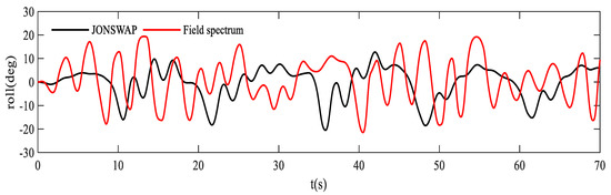
Figure 12.
Time series of the rolling of slender cylinder.
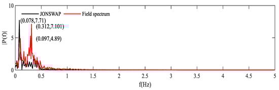
Figure 13.
Frequency curve of rolling of slender cylinder.
6. Conclusions
According to the Longuet-Higgins theory, the method of interpolating and discretizing the field wave spectrum during typhoon was discussed to simulate the three-dimensional typhoon wave motion characteristics. On this basis, considering the directional spectrum, the wave surface, the velocity of water particles, and the acceleration of water particles were emphatically analyzed, which are the basis for using Morison equation to calculate the force and motion of marine floating structures. The main conclusions are summarized as follows.
- (1)
- The field wave spectrum of Typhoon Talim is a dual peak spectrum. The spectrum width of main peak is closer to the improved JONSWAP spectrum, and the secondary peak is smaller than the calculated value by the dual peak spectrum of Ochi-Hubble.
- (2)
- There are small periodic waves on the typhoon wave surface, that is, small-period waves between the peaks and troughs of large-period waves, which may increase the resonance of floating structures and the damage of mooring system.
- (3)
- The magnitude and direction of velocity vector of the water particle on typhoon wave surface have no correlation with the position of the wave crest and trough. The wave water particle velocity calculated by the typhoon Talim simulation variations are ±1.7 m/s, and the water particle acceleration variations are ±2.5 m/s2.
- (4)
- According to the Morison equation, the forces acting on a moored slender cylinder (it is a simplified marine buoy or spar platform) can be calculated under typhoon waves. The keypoint of establishing a coupling calculation model is the calculation of the velocity distribution field as well as acceleration distribution field of the water particle. Under action of the typhoon waves using the field wave spectrum, the rotation angle of moored slender cylinder is more likely to resonate with the secondary peak frequency in the wave spectrum. The response frequency of rotation angle of the JONSWAP spectrum and field spectrum is obvious difference. The numerical simulation method of typhoon wave proposed in this study can be well applied to the hydrodynamic characteristics analysis of moored structures.
Author Contributions
Conceptualization, C.L. and Z.D.; methodology, Y.P.; software, Y.P.; validation, C.L.; formal analysis, C.L., Z.D. and Y.P.; investigation, Y.Z.; resources, Y.Z.; data curation, C.L.; writing—original draft preparation, C.L.; writing—review and editing, C.L., Z.D. and Y.P.; visualization, Y.P.; supervision, Z.D. All authors have read and agreed to the published version of the manuscript.
Funding
This study was funded by the National Natural Science Foundation of China (No.52101330 and No.42006175).
Institutional Review Board Statement
Not applicable.
Informed Consent Statement
Not applicable.
Data Availability Statement
Not applicable.
Conflicts of Interest
The authors declare no conflict of interest.
References
- Feng, X.R.; Yang, D.Z.; Yin, B.S.; Li, M.J. The change and trend of the typhoon waves in Zhejiang and Fujian coastal areas of China. Oceanol. Et Limnol. Sincia 2018, 49, 233–241. (In Chinese) [Google Scholar]
- Goda, Y. A Comparative Review on the Functional Forms of Directional Wave Spectrum. Coast. Eng. J. 1999, 41, 1–20. [Google Scholar] [CrossRef]
- Wang, S.Q.; Liang, B.C. Wave Mechanics for Ocean Engineering; China Ocean University Press: Qingdao, China, 2013; pp. 107–120. [Google Scholar]
- Chen, W.B.; Chen, H.; Hsiao, S.C.; Chang, C.H.; Lin, L.Y. Wind forcing effect on hindcasting of typhoon-driven extreme waves. Ocean. Eng. 2019, 188, 106260. [Google Scholar] [CrossRef]
- Hsiao, S.-C.; Chen, H.; Wu, H.-L.; Chen, W.-B.; Chang, C.-H.; Guo, W.-D.; Chen, Y.-M.; Lin, L.-Y. Numerical Simulation of Large Wave Heights from Super Typhoon Nepartak (2016) in the Eastern Waters of Taiwan. J. Mar. Sci. Eng. 2020, 8, 217. [Google Scholar] [CrossRef] [Green Version]
- Wang, Y.; Tu, X.; Jiang, L.; Fang, Y.; Xu, B.; Ningbo Meteorological Observatory; Ningbo Meteorological Service Center; Xiangshan Meteorological Bureau. Analysis of wave characteristics along Zhejiang coast during typhoon “Lekima”. J. Meteorol. Sci. 2020, 40, 97–105. [Google Scholar]
- Zhou, Y.; Ye, Q.; Yang, B.; Bai, X.; Yan, D. Wave Characteristics in the Bay During Typhoons and Its Effect on Mooring Ships. Shipbuilding of China. Shipbuild. China 2020, 61, 216–227. (In Chinese) [Google Scholar]
- Li, Z.; Hou, Y.; Li, S.; Li, J. Characteristics of wave field in the yellow sea and the bohai sea under the influence of two typ-ical typhoons. Oceanol. Et Limnol. Sincia 2021, 52, 51–65. (In Chinese) [Google Scholar]
- Mo, D.; Liu, Y.; Hou, Y.; Liu, Z. Bimodality and growth of the spectra of typhoon-generated waves in northern South China Sea. Acta Oceanol. Sin. 2019, 38, 70–80. [Google Scholar] [CrossRef]
- Latheef, M.; Abdullah, M.N.; Jupri, M.F.M. Observed spectrum in the South China Sea during storms. Ocean Dyn. 2020, 70, 353–364. [Google Scholar] [CrossRef]
- Zhou, Y.; Ye, Q.; Shi, W.; Yang, B.; Song, Z.; Yan, D. Wave characteristics in the nearshore waters of Sanmen bay. Appl. Ocean Res. 2020, 101, 102236. [Google Scholar] [CrossRef]
- Chang, T.Y.; Chen, H.; Hsiao, S.C.; Wu, H.L.; Chen, W.B. Numerical Analysis of the Effect of Binary Typhoons on Ocean Surface Waves in Wa-ters Surrounding Taiwan. Front. Mar. Sci. 2021, 8, 749185. [Google Scholar] [CrossRef]
- Wei, K.; Imani, H.; Qin, S. Parametric Wave Spectrum Model for Typhoon-Generated Waves Based on Field Measurements in Nearshore Strait Water. J. Offshore Mech. Arct. Eng. 2021, 143, 1–36. [Google Scholar] [CrossRef]
- Strekalov, S.S.; Tsyploukhin, V.P.; Massel, S.T. Structure of sea wave frequency spectrum. Coast. Eng. Proc. 1972, 1, 14. [Google Scholar] [CrossRef] [Green Version]
- Ochi, M.K.; Hubble, E.N. Six-Parameter wave spectra. Coast. Eng. Proc. 1976, 1, 301–327. [Google Scholar] [CrossRef]
- Guedeos, S.C. Representation of double-peaked sea wave spectra. Ocean. Eng. 1984, 11, 185–207. [Google Scholar] [CrossRef]
- Panahi, R.; Ghasemi, A.K.; Shafieefar, M. Development of a bi-modal directional wave spectrum. Ocean Eng. 2015, 105, 104–111. [Google Scholar] [CrossRef]
- Akbari, H.; Panahi, R.; Amani, L. A double-peaked spectrum for the northern parts of the Gulf of Oman: Revisiting extensive field measurement data by new calibration methods. Ocean Eng. 2019, 180, 187–198. [Google Scholar] [CrossRef]
- Golpira, A.; Panahi, R.; Shafieefar, M. Developing families of Ochi-Hubble spectra for the northern parts of the Gulf of Oman. Ocean Eng. 2019, 178, 345–356. [Google Scholar] [CrossRef]
- Fang, X.H.; Xiao, L. Directional spectrum analysis of internal waves in the sea off Sydney, Australia. Coast. Eng. J. 1991, 41, 15–24. [Google Scholar]
- Wang, L.M.; Guo, A.F.; Pei, F. Numerical simulation of sea surface directional wave spectra under typhoon wind forcing. J. Hydrodyn. 2008, 20, 776–783. [Google Scholar]
- Portilla-Yandún, J.; Barbariol, F.; Benetazzo, A.; Cavaleri, L. On the statistical analysis of ocean wave directional spectra. Ocean Eng. 2019, 189, 106361. [Google Scholar] [CrossRef]
- Ribeiro, P.J.C.; Henriques, J.C.C.; Campuzano, F.J.; Gato, L.M.C.; Falcão, A.F.O. A new directional wave spectra characterization for offshore renewable energy applications. Energy 2020, 213, 118828. [Google Scholar] [CrossRef]
- Sun, J.; Guan, C.L. Parameterized first-guess spectrum method for retrieving directional spectrum of swell-dominated waves and huge waves from SAR images. Chine J. Oceanol. Limnol. 2006, 24, 12–20. [Google Scholar]
- Hou, W.; Zhang, R.; Zhang, P.; Xi, Y.; Ma, Q. Wave Characteristics and Berthing Capacity Evaluation of the Offshore Fishing Port under the Influence of Typhoons. Appl. Ocean Res. 2020, 106, 102447. [Google Scholar] [CrossRef]
- Liu, G.; Cui, K.; Jiang, S.; Kou, Y.; You, Z.; Yu, P. A new empirical distribution for the design wave heights under the impact of typhoons. Appl. Ocean. Res. 2021, 111, 102679. [Google Scholar] [CrossRef]
- Abdolali, A.; Roland, A.; van der Westhuysen, A.; Meixner, J.; Chawla, A.; Hesser, T.J.; Smith, J.M.; Sikiric, M.D. Large-scale hurricane modeling using domain decomposition paral-lelization and implicit scheme implemented in WAVEWATCH III wave model. Coast. Eng. 2020, 157, 103656. [Google Scholar] [CrossRef]
- Zhou, Y.; Li, Z.; Pan, Y.; Bai, X.; Wei, D. Distribution characteristics of waves in Sanmen Bay based on field observation. Ocean Eng. 2021, 229, 108999. [Google Scholar] [CrossRef]
- Wu, G.; Liang, Y.; Xu, S. Numerical computational modeling of random rough sea surface based on JONSWAP spectrum and Donelan directional function. Concurr. Comput. Pr. Exp. 2019, 33, e5514. [Google Scholar] [CrossRef]
- Longuet-Higgins, M.S. Statistical properties of wave groups in a random sea state. Statistical Properties of Wave Groups in a Random Sea State. Philos. Trans. R. Soc. A Math. Phys. Eng. Sci. 1984, 312, 219–250. [Google Scholar]
- Radhakrishnan, S.; Datla, R.; Hires, R.I. Theoretical and experimental analysis of tethered buoy instability in gravity waves. Ocean. Eng. 2007, 34, 261–274. [Google Scholar] [CrossRef]
- Morison, J.R.; Johnson, J.W.; Schaaf, S.A. The force exerted by surface waves on piles. J. Pet. Technol. 1950, 2, 149–154. [Google Scholar] [CrossRef]
- Pan, Y.; Tong, H.; Zhou, Y.; Liu, C.; Xue, D. Numerical Simulation Study on Environment-Friendly Floating Reef in Offshore Ecological Belt under Wave Action. Water 2021, 13, 2257. [Google Scholar] [CrossRef]
- Zhu, X.; Yoo, W.S. Numerical modeling of a spar platform tethered by a mooring cable. Chin. J. Mech. Eng.-Ing. 2015, 28, 785–792. [Google Scholar] [CrossRef]
- Zhu, X.; Yoo, W.S. Dynamic analysis of a floating spherical buoy fastened by mooring cables. Ocean Eng. 2016, 121, 462–471. [Google Scholar] [CrossRef]
- Nussbaumer, H.J. The Fast Fourier Transform[M]//Fast Fourier Transform and Convolution Algorithms; Springer: Berlin/Heidelberg, Germany, 1981; pp. 80–111. [Google Scholar]
Publisher’s Note: MDPI stays neutral with regard to jurisdictional claims in published maps and institutional affiliations. |
© 2022 by the authors. Licensee MDPI, Basel, Switzerland. This article is an open access article distributed under the terms and conditions of the Creative Commons Attribution (CC BY) license (https://creativecommons.org/licenses/by/4.0/).