
Prisoners of Scale: Downscaling Community Resilience Measurements for Enhanced Use

 , , and
Abstract
:1. Introduction
2. Materials and Methods
2.1. Index Construction Methodology
2.2. Gulf Coast Region Implementation
3. Index Construction Results
3.1. Exploratory Factor Analysis
3.2. Reliability Testing for Capitals
3.3. Expert Judgement
4. TBRIC Implementation and Analysis
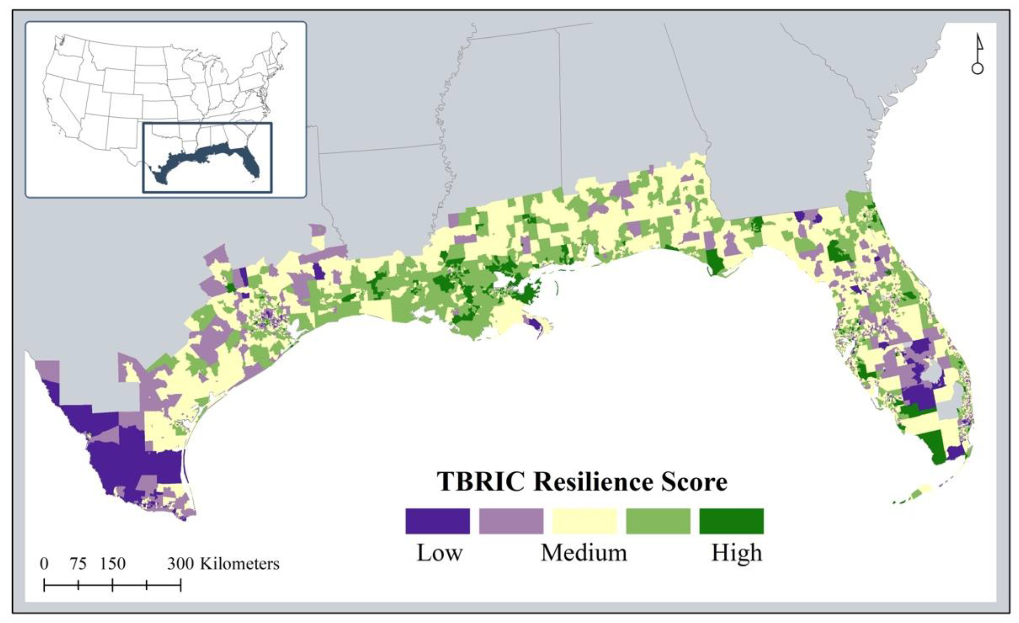
4.1. Final TBRIC Configuration
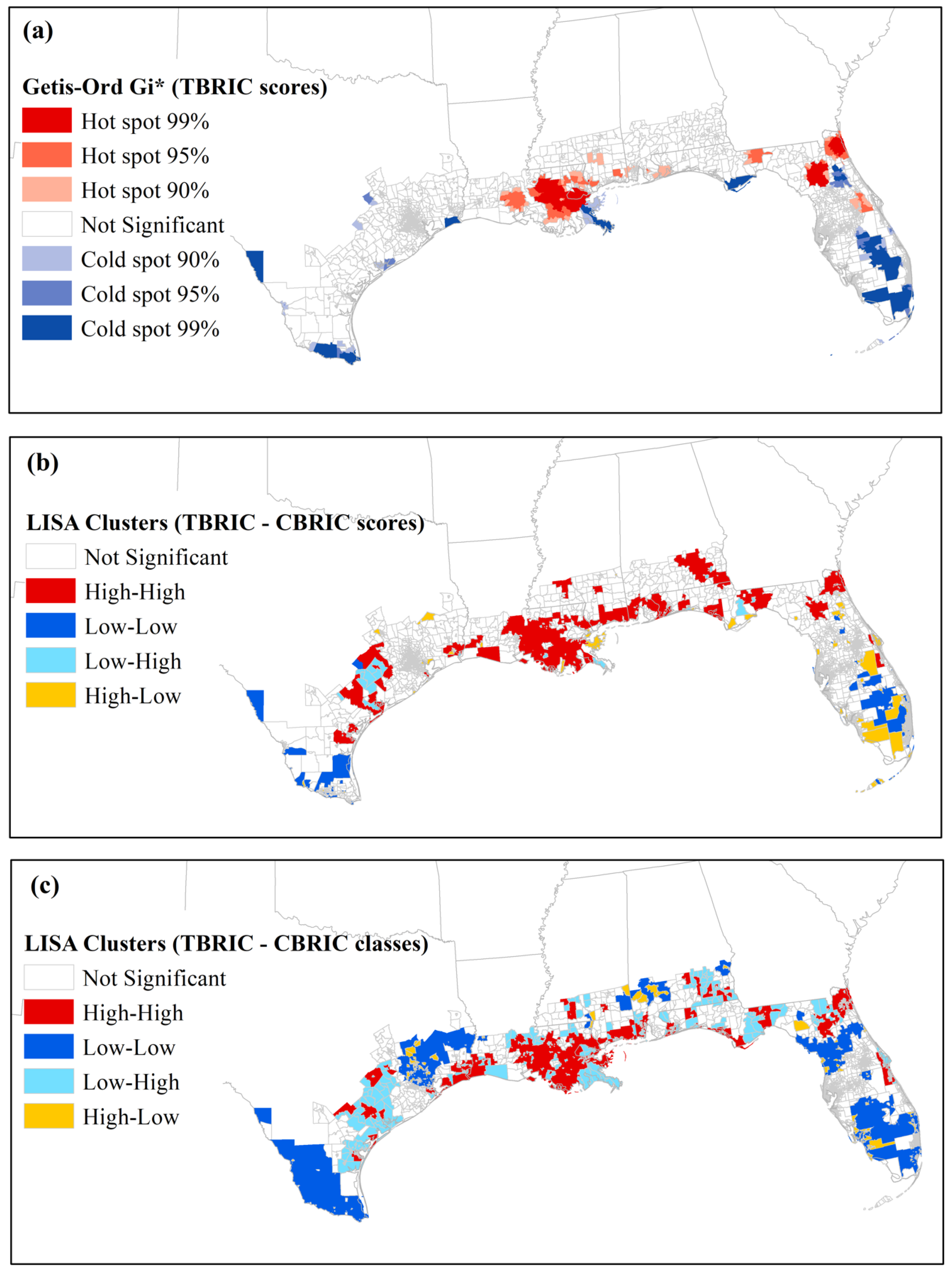
4.2. Scale Effects: TBRIC vs. CBRIC
5. Discussion and Conclusions
Author Contributions
Funding
Institutional Review Board Statement
Informed Consent Statement
Data Availability Statement
Acknowledgments
Conflicts of Interest
Appendix A

| Variable | Calculation | Changes from Original |
|---|---|---|
| Social Resilience | ||
| Educational equity | Percent population with college education or more | Definitional |
| Age | Percent population between 18 to 65 years old | Definitional |
| Transportation access | Percent households with at least one vehicle | |
| Communication capacity | Percent households with telephone service available | |
| Language competency | Percent population that are proficient English speakers | |
| Non-special needs | Percent population without a sensory, physical, or mental disability | |
| Health coverage | Percent of the population (under 65) with health insurance coverage | |
| Mental health | Psychosocial support facilities per 10 k population | |
| Food access | Food Insecurity Rate (population at 1 mile for urban areas and 10 miles for rural areas) (Inverted) * | New substitute |
| Physician access | Number of physicians per 1000 population | |
| Economic Resilience | ||
| Homeownership | Percent owner-occupied housing units | |
| Employment | Percent labor force employed | |
| Income and equality (Race/Ethnicity) | GINI coefficient of income equality (Inverted) * | |
| Non-dependence on primary and tourism employment | Percent population not employed in farming, fishing, forestry, extractive, and tourism industries | |
| Income and equality (Gender) | Percent of absolute difference between male median annual earnings and female median annual earnings divided by annual income (Inverted) * | Computation |
| Business size I | Ratio of number of large (more than 100 employees) to small (less than 10 employees) businesses | |
| Business size II | Ratio of number of employees to number of establishments | New |
| Multi-purpose retail | Department stores per 1000 population | |
| Energy burden | Energy burden as % income (Inverted) * | New |
| Sales rate | Average sales volume divided by number of businesses | New |
| Building permits | Average number of building permits per 1000 population (5-year average) | New |
| Income to mortgage ratio | Median income to loan ratio | New |
| Military employment | Percent employed Armed Forces | New substitute |
| Institutional Resilience | ||
| Mitigation spending | Average amount ($) mitigation projects for 10-year period per capita | |
| Mitigation cost share | Mitigation cost-share percentage (10-year average) | New |
| Flood insurance coverage | Percent of housing units covered by NFIP policies | |
| Incorporated areas | Percent incorporated | New |
| Jurisdictional uniformity | Number of governments & special districts per 10 k persons | |
| Local disaster training | Number of Citizen Corps programs (local and county) per 1000 people | |
| Governance connectivity and performance regimes | Proximity to county seat (Travel time from centroid of census tract to county seat; inverted; closer is more resilient) (Inverted) * | New substitute |
| Population Stability | Absolute value of population change base year/current year | |
| Nuclear accident planning | Census tracts within 10 miles of nuclear power plant (Binary 0/1) | |
| Social assistance services | Number of social assistance services per 1000 population | New |
| Community housing and emergency and relief services | Number of community housing and emergency and relief services per 1000 population | New |
| Emergency services | Number of emergency services per 1000 population | New |
| Housing/Infrastructural Resilience | ||
| Housing type | Percent housing units that are not mobile homes | |
| Temporary housing availability | Vacant rental units per 1000 population | |
| Medical care capacity | Hospital beds per 1000 population; Buffer 10 mile for hospitals (to match food access buffer), measured by population of tracts within the buffer then assigned to the tracts, for buffers more than 1, the average is assigned to the underlying tract | Computation |
| Medical care access | Average travel time to hospitals from tract centroid | New |
| Access/Evacuation potential | Intersection density (n_real nodes/tract_area_sq miles) | New substitute |
| Housing age | Percent housing units built before 1970 or after 2000 | New substitute |
| Sheltering needs | Number of hotels/motels per 1000 population | |
| School restoration potential | Number of public schools per 1000 population | |
| Bridge rating | Average sufficiency rating of all bridges within tract | New |
| Dam age | Average age of dams within tract (Inverted) * | New |
| Tax-exempt organizations | Tax-exempt organizations per 1000 population | New |
| Internet Access--connectivity | Number of actual connections per 1000 households | New |
| Internet Access--speed | Percent population with broadband internet subscription | New substitute |
| Community Capital | ||
| Place attachment (not recent immigrants) | Population who are foreign-born and moved to US in previous 5 years per 1000 population | |
| Place attachment (nativity/tenure) | Percent population born in a state that still resides in that state | |
| Political engagement | Percent voter participation in a Presidential election (Precinct level data) | |
| Social capital—religion | Number of religious organizations per 1000 population | |
| Social capital—civic involvement | Number of civic organizations per 1000 population | |
| Social capital—volunteerism | AmeriCorps volunteers per 1000 population | New substitute |
| Community engagement | Number of art, entertainment, and recreation establishments per 1000 population | New |
| Place security/Evictions | Evictions per 1000 population (Inverted) * | New |
| Sense of security | Crime rate (property and violent crime), 5-year average, per 1000 population (Inverted) * | New |
| Cultural heritage | Museums, historical sites, and similar institutions per 1000 population | New |
| Environmental Resilience | ||
| Natural buffers | Percent Land in wetlands | |
| Energy use | Energy Use (megawatt hours) per Energy Consumer | |
| Pervious surfaces | Average Percent Perviousness | |
| Water supply stress | Domestic per capita use self-supply (in gallons/person/day) | New substitute |
| Flood risk | Percent land in flood plain | New |
| Urban flooding | Average Flash Flood Potential Index (FFPI) value (Inverted) * | New |
| Air quality-particulate matter | Average PM value of particulates less than 2.5 (PM2.5) by census tract from 1998 to 2016 (Inverted) * | New |
| Toxic facilities | Number of Superfund or LQG hazardous waste facilities in census tract per 1000 population (Inverted) * | New |
| Federal Registry Service sites | All FRS sites in census tract per 1000 population (Inverted) * | New |
| Water quality risk | NPDES point source pollution facilities in census tract per 1000 population (Inverted) * | New |
| Air polluting facilities | Number of critical/hazardous air polluting facilities in census tract per 1000 population (Inverted) * | New |
| Change in pervious surfaces | Average Percent Perviousness change 2006–2016 | New |
| Open space | Percent land in parks | New |
| Local food environment | Farmers’ markets per 1000 population (2018) | New |
Appendix B
| Pedigree Results by Variable Including Average Rate and Range of Rating’s Epistemic Uncertainty * | ||||
|---|---|---|---|---|
| Variable name | Applicability for local scale (1–2) | Statistical contribution (1–3) | Accessibility (1–3) | Simplicity for replication (1–3) |
| Educational equity | 2 (±0) | 3 (±0) | 3 (±0) | 3 (±0) |
| Age | 2 (±0) | 3 (±0) | 3 (±0) | 3 (±0) |
| Transportation access | 2 (±0) | 3 (±0) | 3 (±0) | 3 (±0) |
| Communication capacity | 2 (±0) | 3 (±0) | 3 (±0) | 3 (±0) |
| Language competency | 2 (±0) | 3 (±0) | 3 (±0) | 2.5 (±0.5) |
| Special needs | 2 (±0) | 3 (±0) | 3 (±0) | 3 (±0) |
| Health coverage | 2 (±0) | 3 (±0) | 3 (±0) | 3 (±0) |
| Mental health | 2 (±0) | 2.5 (±0.5) | 3 (±0) | 2.5 (±0.5) |
| Food access | 2 (±0) | 1.5 (±0.5) | 3 (±0) | 2.5 (±0.5) |
| Health access | 2 (±0) | 3 (±0) | 3 (±0) | 2.5 (±0.5) |
| Housing capital | 2 (±0) | 2.5 (±0.5) | 3 (±0) | 3 (±0) |
| Employment | 2 (±0) | 3 (±0) | 3 (±0) | 2.5 (±0.5) |
| Income and equality (Race/Ethnicity) | 2 (±0) | 1.5 (±0.5) | 3 (±0) | 3 (±0) |
| Non-dependence on primary/tourism employment | 1.5 (±0.5) | 2 (±0) | 3 (±0) | 2.5 (±0.5) |
| Income and equality (Gender) | 2 (±0) | 3 (±0) | 3 (±0) | 3 (±0) |
| Business size I | 1.5 (±0.5) | 3 (±0) | 2.5 (±0.5) | 2.5 (±0.5) |
| Business size II | 1.5 (±0.5) | 3 (±0) | 2.5 (±0.5) | 2.5 (±0.5) |
| Multi-purpose retail | 1.5 (±0.5) | 2 (±0) | 2.5 (±0.5) | 2.5 (±0.5) |
| Energy burden | 2 (±0) | 2.5 (±0.5) | 3 (±0) | 3 (±0) |
| Building permit | 2 (±0) | 2 (±0) | 3 (±0) | 2.5 (±0.5) |
| Sales rate | 2 (±0) | 3 (±0) | 2.5 (±0.5) | 2.5 (±0.5) |
| Income to mortgage ratio | 2 (±0) | 2 (±1) | 3 (±0) | 3 (±0) |
| Military employment | 2 (±0) | 2 (±0) | 3 (±0) | 3 (±0) |
| Mitigation spending | 1.5 (±0.5) | 3 (±0) | 3 (±0) | 2.5 (±0.5) |
| Mitigation cost share | 1.5 (±0.5) | 3 (±0) | 3 (±0) | 2.5 (±0.5) |
| Flood insurance coverage | 1.5 (±0.5) | 2 (±0) | 3 (±0) | 2.5 (±0.5) |
| Incorporated areas | 1 (±0.5) | 1 (±0.5) | 1 (±0.5) | 1 (±0.5) |
| Jurisdictional uniformity | 1.5 (±0.5) | 3 (±0) | 2 (±0) | 3 (±0) |
| Local disaster training | 2 (±0) | 3 (±0) | 3 (±0) | 2 (±0) |
| Performance regimes—Distance to county seat | 2 (±0) | 2 (±0) | 1.5 (±0.5) | 1 (±0) |
| Social assistance services | 2 (±0) | 3 (±0) | 2 (±0) | 2 (±0) |
| Community housing and emergency services | 2 (±0) | 3 (±0) | 2 (±0) | 2 (±0) |
| Population Stability | 2 (±0) | 3 (±0) | 3 (±0) | 3 (±0) |
| Nuclear Accident Planning | 1 (±0) | 1 (±0) | 3 (±0) | 2 (±0) |
| Emergency Services (Police/Fire) | 2 (±0) | 3 (±0) | 3 (±0) | 2 (±0) |
| Housing type | 2 (±0) | 3 (±0) | 3 (±0) | 3 (±0) |
| Temporary Housing Availability | 2 (±0) | 2.5 (±0.5) | 3 (±0) | 3 (±0) |
| Medical capacity | 2 (±0) | 2.5 (±0.5) | 3 (±0) | 1.5 (±0.5) |
| Medical access | 2 (±0) | 3 (±0) | 2.5 (±0.5) | 1 (±0) |
| Access/Evacuation potential | 2 (±0) | 3 (±0) | 1 (±0) | 1.5 (±0.5) |
| Housing age | 2 (±0) | 3 (±0) | 3 (±0) | 3 (±0) |
| Sheltering needs | 2 (±0) | 2.5 (±0.5) | 2 (±0) | 3 (±0) |
| Recovery potential | 2 (±0) | 2.5 (±0.5) | 3 (±0) | 2.5 (±0.5) |
| Bridge Rating | 2 (±0) | 2.5 (±0.5) | 3 (±0) | 2 (±0) |
| Dam Age | 1.5 (±0.5) | 2.5 (±0.5) | 3 (±0) | 2 (±0) |
| Tax-exempt organizations | 2 (±0) | 2.5 (±0.5) | 2.5 (±0.5) | 2.5 (±0.5) |
| Internet access (2 variables) | 2 (±0) | 2.5 (±0.5) | 2 (±0) | 2.5 (±0.5) |
| Place attachment (recent immigrants) | 2 (±0) | 2 (±1) | 3 (±0) | 3 (±0) |
| Place attachment (nativity/tenure) | 1.5 (±0.5) | 3 (±0) | 3 (±0) | 3 (±0) |
| Political engagement | 1.5 (±0.5) | 3 (±0) | 3 (±0) | 3 (±0) |
| Social capital—religion | 1.5 (±0.5) | 2.5 (±0.5) | 1.5 (±0.5) | 2.5 (±0.5) |
| Social capital—civic involvement | 2 (±0) | 3 (±0) | 2 (±0) | 3 (±0) |
| Social Capital—volunteerism | 2 (±0) | 2 (±0) | 2 (±0) | 3 (±0) |
| Art, entertainment, and recreation centers | 2 (±0) | 2.5 (±0.5) | 2 (±0) | 2.5 (±0.5) |
| Evictions | 2 (±0) | 2 (±0) | 2 (±0) | 3 (±0) |
| Sense of security | 1.5 (±0.5) | 3 (±0) | 2.5 (±0.5) | 2.5 (±0.5) |
| Cultural heritage | 2 (±0) | 2 (±0) | 2 (±0) | 3 (±0) |
| Natural buffers | 1.5 (±0.5) | 3 (±0) | 2 (±1) | 2 (±1) |
| Energy use | 1.5 (±0.5) | 1 (±0) | 3 (±0) | 3 (±0) |
| Pervious surfaces | 2 (±0) | 2 (±1) | 2 (±0) | 2 (±0) |
| Water supply stress | 1.5 (±0.5) | 2 (±0) | 2.5 (±0.5) | 2.5 (±0.5) |
| Flood risk | 1.5 (±0.5) | 1 (±0) | 2 (±1) | 2 (±1) |
| Urban flooding | 1.5 (±0.5) | 1 (±0) | 1 (±0) | 1 (±0) |
| Air quality-particulate matter | 2 (±0) | 1.5 (±0.5) | 2.5 (±0.5) | 2 (±1) |
| Toxic facilities | 2 (±0) | 2 (±0) | 3 (±0) | 2.5 (±0.5) |
| FRS sites | 2 (±0) | 2 (±1) | 3 (±0) | 2.5 (±0.5) |
| Water quality risk | 2 (±0) | 2.5 (±0.5) | 3 (±0) | 2.5 (±0.5) |
| Air polluting facilities | 2 (±0) | 2.5 (±0.5) | 3 (±0) | 2.5 (±0.5) |
| Change in pervious surfaces 2006–2016 | 2 (±0) | 2.5 (±0.5) | 2.5 (±0.5) | 2.5 (±0.5) |
| Open space | 2 (±0) | 3 (±0) | 2.5 (±0.5) | 2.5 (±0.5) |
| Local food environment | 2 (±0) | 2.5 (±0.5) | 3 (±0) | 3 (±0) |
| * Rating guide | Applicability for local scale | Statistical contribution | Accessibility | Simplicity for replication |
| 1 (Not applicable) | 1 (No contribution) | 1 (Difficult to find/clean data) | 1 (High computational skill required) | |
| 2 (Applicable) | 2 (Low significance) | 2 (Time-consuming but available) | 2 (Medium computational skill required) | |
| 3 (Significant) | 3 (Easily accessible) | 3 (Easily computable) | ||
References
- National Research Council. Disaster Resilience: A National Imperative; National Academies Press: Washington, DC, USA, 2012. [Google Scholar]
- Folke, C.; Biggs, R.; Norström, A.; Reyers, B.; Rockström, J. Social-ecological resilience and biosphere-based sustainability science. Ecol. Soc. 2016, 21, 41. [Google Scholar] [CrossRef]
- Meerow, S.; Newell, J.; Stults, M. Defining urban resilience: A review. Landsc. Urban Plan. 2016, 147, 38–49. [Google Scholar] [CrossRef]
- Cutter, S.L. Urban risks and resilience, Chapter 13. In Urban Informatics; Shi, W., Ed.; Springer: Berlin/Heidelberg, Germany, 2021. [Google Scholar]
- Woodruff, S.; Bowman, A.O.; Hannibal, B.; Sansom, G.; Portney, K. Urban resilience: Analyzing the policies of U.S. cities. Cities 2021, 115, 103239. [Google Scholar] [CrossRef]
- Cox, R.S.; Hamlen, M. Community disaster resilience and the Rural Resilience Index. Amer. Behav. Sci. 2015, 59, 220–237. [Google Scholar] [CrossRef]
- Jurjonas, M.; Seekamp, E. Rural coastal community resilience: Assessing a framework in eastern North Carolina. Ocean Coast Manag. 2017, 162, 137–150. [Google Scholar] [CrossRef]
- Van de Lindt, J.W.; Peacock, W.G.; Mitrani-Reiser, J.; Rosenheim, N.; Deniz, D.; Dillard, M.; Tomiczek, T.; Koliou, M.; Graettinger, A.; Crawford, P.S.; et al. Community Resilience-Focused Technical Investigation of the 2016 Lumberton, North Carolina, Flood: An Interdisciplinary Approach. Nat. Hazards Rev. 2020, 21, 3. [Google Scholar] [CrossRef]
- Cutter, S.L.; Ash, K.D.; Emrich, C.T. Urban-rural differences in disaster resilience. Ann. Am. Assoc. Geogr. 2016, 106, 1236–1252. [Google Scholar] [CrossRef]
- Nguyen, R.L.; Akerkar, R. Modelling, measuring, and visualizing community resilience: A systematic review. Sustainability 2020, 12, 7896. [Google Scholar] [CrossRef]
- Ruth, M.; Goessling-Reisemann, S. Handbook on Resilience of Socio-Technical Systems; Elgar: Cheltenham, UK, 2019. [Google Scholar]
- Garcia, E.J.; Vale, B. Unraveling Sustainability and Resilience in the Built Environment; Routledge: London, UK, 2017. [Google Scholar]
- Bakkensen, L.A.; Fox-Lent, C.; Read, L.K.; Linkov, I. Validating Resilience and Vulnerability Indices in the Context of Natural Disasters. Risk Anal. 2017, 37, 982–1004. [Google Scholar] [CrossRef] [PubMed] [Green Version]
- Carvalhaes, T.M.; Chester, M.V.; Reddy, A.T.; Allenby, B.R. An Overview & Synthesis of Disaster Resilience Indices from a Complexity Perspective. Intl. J. Disaster Risk Reduct. 2021, 57, 102165. [Google Scholar]
- Johnson, P.W.; Brady, C.E.; Philip, C.; Baroud, H.; Camp, J.V.; Abkowitz, M. A factor analysis approach toward reconciling community vulnerability and resilience indices for natural hazards. Risk Anal. 2020, 40, 1795–1810. [Google Scholar] [CrossRef] [PubMed]
- National Academies of Sciences, Engineering, and Medicine. Building and Measuring Community Resilience: Actions for Communities and the Gulf Research Program; National Academies Press: Washington, DC, USA, 2019. [Google Scholar]
- Cutter, S.L.; Ash, K.D.; Emrich, C.T. The Geographies of Community Disaster Resilience. Glob. Environ. Chang. 2014, 29, 65–77. [Google Scholar] [CrossRef]
- Cutter, S.L.; Derakhshan, S. Temporal and Spatial Change in Disaster Resilience in U.S. Counties, 2010–2015. Environ. Hazards 2018, 19, 10–29. [Google Scholar] [CrossRef]
- The National Risk Index. Federal Emergency Management Agency (FEMA). Available online: https://hazards.fema.gov/nri/ (accessed on 20 April 2022).
- Weichselgartner, J.; Kelman, I. Geographies of Resilience. Prog. Hum. Geogr. 2014, 39, 249–267. [Google Scholar] [CrossRef] [Green Version]
- Openshaw, S. The Modifiable Areal Unit Problem, Concepts and Techniques in Modern Geography. Available online: https://www.uio.no/studier/emner/sv/iss/SGO9010/openshaw1983.pdf (accessed on 15 April 2022).
- Robinson, W.S. Ecological Correlations, and the Behavior of Individuals. Am. Sociol. Rev. 1950, 15, 351–357. [Google Scholar] [CrossRef]
- Nelson, J.K.; Brewer, C.A. Evaluating data stability in aggregation structures across spatial scales: Revisiting the modifiable areal unit problem. Cartogr. Geogr. Inf. Sci. 2017, 44, 35–50. [Google Scholar] [CrossRef]
- Kwan, M.P. The Uncertain Geographic Context Problem. Ann. Assoc. Am. Geographers. 2012, 102, 958–968. [Google Scholar] [CrossRef]
- Frazier, T.G.; Thompson, C.M.; Dezzani, R.J.; Butsick, D. Spatial and Temporal Quantification of Resilience at the Community Scale. Appl. Geogr. 2013, 42, 95–107. [Google Scholar] [CrossRef]
- Hong, B.; Bonczak, B.J.; Gupta, A.; Kontokosta, C.E. Measuring Inequality in Community Resilience to Natural Disasters Using Large-Scale Mobility Data. Nat. Commun. 2021, 12, 1870. [Google Scholar] [CrossRef]
- Cardoni, A.; Zamani Noori, A.; Greco, R.; Cimellaro, G.P. Resilience assessment at the regional level using census data. Intl. J. Disaster Risk Reduct. 2021, 55, 102059. [Google Scholar] [CrossRef]
- Ciccotti, L.; Rodrigues, A.C.; Boscov, M.E.G.; Gunther, W.M.R. Building indicators of community resilience to disasters in Brazil: A participatory approach. Ambient. Soc. 2020, 23, e01231. [Google Scholar] [CrossRef]
- Scherzer, S.; Lujala, P.; Rød, J.K. A community resilience index for Norway: An adaptation of the Baseline Resilience Indicators for Communities (BRIC). Intl. J. Disaster Risk Reduct. 2019, 36, 101107. [Google Scholar] [CrossRef]
- Singh-Petersen, L.; Salmon, P.; Goode, N.; Gallina, J. Translation and evaluation of the baseline resilience indicators for communities on the sunshine coast, Queensland, Australia. Intl. J. Disaster Risk Reduct. 2014, 10 Pt A, 116–126. [Google Scholar] [CrossRef]
- Cutter, S.L.; Emrich, C.T.; Mitchell, J.T.; Piegorsch, W.W.; Smith, M.M.; Weber, L. Hurricane Katrina, and the Forgotten Coast of Mississippi; Cambridge University Press: Cambridge, UK, 2014. [Google Scholar]
- Cutter, S.L.; Emrich, C.T.; Gall, M.; Harrison, S.; McCaster, R.R.; Derakhshan, S.; Pham, E. Existing Longitudinal Data, and Systems for Measuring the Human Dimensions of Resilience, Health and Well-being in the Gulf Coast. Available online: https://www.nationalacademies.org/_cache_80ac/content/4885770000234289.pdf (accessed on 10 February 2022).
- Cronbach, L.J. Coefficient alpha and the internal structure of tests. Psychometrika 1951, 16, 297–334. [Google Scholar] [CrossRef] [Green Version]
- Getis, A.; Ord, J.K. The Analysis of Spatial Association by Use of Distance Statistics. Geogr. Anal. 1992, 24, 189–206. [Google Scholar] [CrossRef]
- Anselin, L.; Syabri, I.; Kho, Y. GeoDa: An Introduction to Spatial Data Analysis. Geogr. Anal. 2006, 38, 5–22. [Google Scholar] [CrossRef]
- Office for Coastal Management, NOAA, Defining Coastal Counties. Available online: https://coast.noaa.gov/digitalcoast/training/defining-coastal-counties.html (accessed on 25 January 2022).
- U.S. Census Bureau. Economic Census (2002–2017). Available online: https://guides.loc.gov/census-connections/economic-census/2002-2017 (accessed on 10 February 2022).
- Rabby, Y.W.; Hossain, M.B.; Hasan, M.U. Social vulnerability in the coastal region of Bangladesh: An investigation of social vulnerability index and scalar change effects. Intl. J. Disaster Risk Reduct. 2019, 41, 101329. [Google Scholar] [CrossRef]
- Paegelow, M.; Quense, J.; Peltier, A.; Henríquez Ruiz, C.; Le Goff, L.; Arenas Vásquez, F.; Antoine, J.-M. Water vulnerabilities mapping: A multi-criteria and multi-scale assessment in central Chile. Water Policy 2022, 24, 159–178. [Google Scholar] [CrossRef]

| Component | % Variance Explained | Dominant Variables * | Component Loading |
|---|---|---|---|
| 1 | 17.469 | Mitigation spending | 0.992 |
| Emergency services (police/fire) | 0.984 | ||
| Civic involvement | 0.979 | ||
| Building permits | 0.971 | ||
| Temporary housing availability | 0.938 | ||
| Tax-exempt organizations | 0.933 | ||
| Cultural heritage | 0.907 | ||
| Local disaster training | 0.880 | ||
| Art, entertainment, recreation centers | 0.637 | ||
| Energy burden | −0.664 | ||
| Air polluting facilities | −0.965 | ||
| Toxic facilities | −0.976 | ||
| Water quality risk | −0.987 | ||
| FRS sites | −0.989 | ||
| 2 | 8.488 | Educational equity | 0.716 |
| Internet access (speed) | 0.819 | ||
| Transportation access | 0.690 | ||
| Internet access (connectivity) | 0.614 | ||
| Physician access | 0.573 | ||
| Special needs | 0.576 | ||
| Health insurance coverage | 0.560 | ||
| 3 | 7.921 | Access/evacuation potential | 0.756 |
| Medical access | 0.660 | ||
| Housing type | 0.549 | ||
| Housing capital | −0.504 | ||
| Natural buffers, wetlands | −0.618 | ||
| Pervious surfaces | −0.740 | ||
| 4 | 5.032 | Language competency | 0.844 |
| Place attachment (recent immigrants) | 0.837 | ||
| Health insurance coverage | 0.593 | ||
| Energy use | −0.632 | ||
| 5 | 4.616 | Political engagement | 0.494 |
| Air quality (particulate matter) | 0.493 | ||
| Income to mortgage ratio | −0.661 | ||
| Water supply | −0.700 | ||
| Place attachment (nativity/tenure) | −0.746 | ||
| 6 | 3.231 | Sheltering needs | 0.977 |
| Multi-purpose retail | 0.975 | ||
| Social assistance services | 0.932 | ||
| Art, entertainment, recreation centers | 0.756 | ||
| 7 | 2.567 | Military employment | 0.521 |
| Age | 0.480 | ||
| Mitigation cost share | 0.477 | ||
| Employment | −0.471 | ||
| 8 | 2.341 | Business size II | 0.578 |
| Business size I | 0.562 | ||
| Sales rate | 0.522 |
| Resilience Category | Number of Indicators | Initial Cronbach’s Alpha TBRIC 2020 |
|---|---|---|
| Social | 10 | 0.425 |
| Economic | 13 | −0.285 |
| Community Capital | 10 | 0.246 |
| Institutional | 11 * | 0.113 |
| Housing/Infrastructural | 13 | 0.310 |
| Environmental | 13 ** | −0.492 |
| Variable | Decision | Rationale |
|---|---|---|
| Incorporated areas | Eliminated | Data limitation/unavailability |
| Nuclear accident planning | Eliminated | Conceptual inapplicability at local scale and statistical insignificance |
| Flood risk | Eliminated | Conceptual inapplicability at local scale and statistical insignificance |
| Urban flooding | Eliminated | Data limitation/unavailability |
| Air quality-particulate matter | Eliminated | Conceptual inapplicability at local scale and statistical insignificance |
| FRS sites | Eliminated | Statistical insignificance |
| Energy use | Eliminated | Statistical insignificance |
| Internet Access (speed) | Reassigned | Moved from infrastructural capital to social capital, based on concept and reliability test performance. Note, the other variable for internet access (number of actual connections per 1000 households) is kept in infrastructural. |
| Language competency | Reassigned | Moved from social capital to community capital, based on concept and reliability test performance. |
| Food access | Reassigned | Moved from social capital to infrastructural capital, based on concept and reliability test performance. |
| Income to mortgage ratio | Reassigned | Moved from economic capital to community capital, based on concept and reliability test performance. |
| Resilience Category | Number of Indicators | Cronbach’s Alpha TBRIC | Inter-item Correlation (Mean) |
|---|---|---|---|
| Social | 9 | 0.699 | 0.236 *** |
| Economic | 12 | −0.103 | 0.009 *** |
| Community Capital | 12 | 0.499 | 0.086 *** |
| Institutional | 10 | 0.213 | 0.087 *** |
| Housing/Infrastructural | 13 | 0.283 | 0.034 *** |
| Environmental | 9 | 0.410 | 0.114 *** |
| TBRIC Total | 65 | 0.456 | 0.019 *** |
| Resilience Category | Number of Indicators | Cronbach’s Alpha CBRIC | Inter-Item Correlation (Mean) |
|---|---|---|---|
| Social | 10 | 0.543 | 0.103 *** |
| Economic | 8 | −0.205 | −0.016 *** |
| Community Capital | 7 | 0.444 | 0.064 *** |
| Institutional | 10 | 0.332 | 0.032 *** |
| Housing/Infrastructural | 9 | 0.415 | 0.072 *** |
| Environmental | 5 | −0.266 | −0.024 *** |
| CBRIC Total | 49 | 0.550 | 0.025 *** |
Publisher’s Note: MDPI stays neutral with regard to jurisdictional claims in published maps and institutional affiliations. |
© 2022 by the authors. Licensee MDPI, Basel, Switzerland. This article is an open access article distributed under the terms and conditions of the Creative Commons Attribution (CC BY) license (https://creativecommons.org/licenses/by/4.0/).
Share and Cite
Derakhshan, S.; Blackwood, L.; Habets, M.; Effgen, J.F.; Cutter, S.L. Prisoners of Scale: Downscaling Community Resilience Measurements for Enhanced Use. Sustainability 2022, 14, 6927. https://doi.org/10.3390/su14116927
Derakhshan S, Blackwood L, Habets M, Effgen JF, Cutter SL. Prisoners of Scale: Downscaling Community Resilience Measurements for Enhanced Use. Sustainability. 2022; 14(11):6927. https://doi.org/10.3390/su14116927
Chicago/Turabian StyleDerakhshan, Sahar, Leah Blackwood, Margot Habets, Julia F. Effgen, and Susan L. Cutter. 2022. "Prisoners of Scale: Downscaling Community Resilience Measurements for Enhanced Use" Sustainability 14, no. 11: 6927. https://doi.org/10.3390/su14116927
APA StyleDerakhshan, S., Blackwood, L., Habets, M., Effgen, J. F., & Cutter, S. L. (2022). Prisoners of Scale: Downscaling Community Resilience Measurements for Enhanced Use. Sustainability, 14(11), 6927. https://doi.org/10.3390/su14116927