Food Preservation within Multi-Echelon Supply Chain Considering Single Setup and Multi-Deliveries of Unequal Lot Size

Abstract

Intricacy of the supply chains for deteriorating products, involving multiple retailers with unequal lot sizes and multiple deliveries is simplified in this article by optimizing the replenishment cycle, investment in preservation technology, and number of deliveries. This study proposes a multi-tier supply chain model consisting of a single manufacturer and multiple retailers. A single-setup multiple deliveries (SSMD) policy is adopted considering the synchronized cycle time of manufacturers with that of retailers and the delivery of unequal lot size for each retailer. Preservation technology is used at retailers to minimize the effects of deterioration in a way that the magnitude of decrease in deterioration reduces for additional investment in preservation technology. A centralized supply chain model is proposed by defining a nonlinear mathematical model for maximizing total profit through an analytical optimization technique and an algorithm. Numerical experiments are exhibited to validate the applications of the provided model. The results exhibit that the proposed preservation policy increases the product’s lifetime and the total profit by reducing the number of shipments/transportation and increasing the lot size. The SSMD policy helps to reduce the preservation cost and increase the total profit. Some managerial insights are provided for the decision makers for applying the proposed model.

1. Introduction

Products that deteriorate with time, for example, food products, tend to create more waste in a shorter period. Carefully carried out surveys estimate that 1.3 billion tons of food are being wasted each year, which is 33% of the total food produced in the world [1]. The food products in different regions of a country or across the globe are retailed at multiple retail stores while being supplied by a single manufacturer. The supply of food products and their storage at retailers are key issues for food supply chains. The provision of food products as fresh as prepared at a reduced price and better service level are challenges for supply chain managers to sustain in an competitive business environment. For supplying fresh food items to multiple locations, a vigilant delivery plan can be effective to consider the retailers’ cycle time and deterioration of products. Considering these facts, a centralized supply chain system comprising a single manufacturer and multiple retailers helps the customers at various locations by providing them fresh food items at reduced prices. Management of such centralized food supply chains, which deteriorate with time, can be simplified by synchronizing the delivery time at retailers [2,3,4,5,6,7,8,9,10].

It is a multifarious assignment to devise a supply chain policy for deteriorating products, where a single manufacturer fulfills the demand for multiple retailers having different stock levels/unequal lot sizes. The system becomes more complex when customer service is given a priority and shortages are not allowed. However, manufacturers can negotiate with retailers to plan their replenishment periods in a way such that their inventory replenishment cycle coincides. In a centralized system, this is more optimal to plan the same time span of inventory replenishment at the retailers’ level. This helps manufacturers to handle the deliveries and plan their transportation activities smoothly and in a synchronized pattern [11].

To avoid losses by deterioration, manufacturers can adopt the policy of multiple shipments/deliveries to the retailers. Smaller lot sizes and frequent inventory replenishments are supportive policies in reducing the effects of deterioration, but these policies increase the transportation cost. The losses due to deterioration can also be minimized by adopting preservation policies for retailers. The preservation adopted for food products provides retailers with more time for selling their products without facing serious deterioration that contributes to the sales revenue and increases the profit. In the presence of preservation for fresh food products at retailers, a larger amount of delivery may be planned, which can reduce the number of shipments and transportation costs. The number of shipments, delivery size, retailers’ cycle time, and amount of preservation effect several component costs and sales revenue; therefore, estimating their optimal values plays a vital role in reducing costs and maximizing profit. A reduced number of shipments increases the profit by reducing the cost of transportation on one side; however on the other side, it decreases the profit by increasing the inventory holding costs at the retailer and by causing more items to deteriorate due to increased cycle time at the retailers’ level. Furthermore, the behavior of sales at each retailer is not necessarily the same due to several geographic, demographic, and marketing reasons. Therefore, customer demand at each retailer is different. Thus, it is more realistic to design unequal replenishment quantities for each retailer. This study satisfies the following research questions.

• What is the set of solutions to optimize deterioration using multiple deliveries and preservation simultaneously?
• Does the SSMD policy affect investment in preservation?
• Does the investment in preservation have any effect on the number of deliveries/shipments within an SSMD setup?
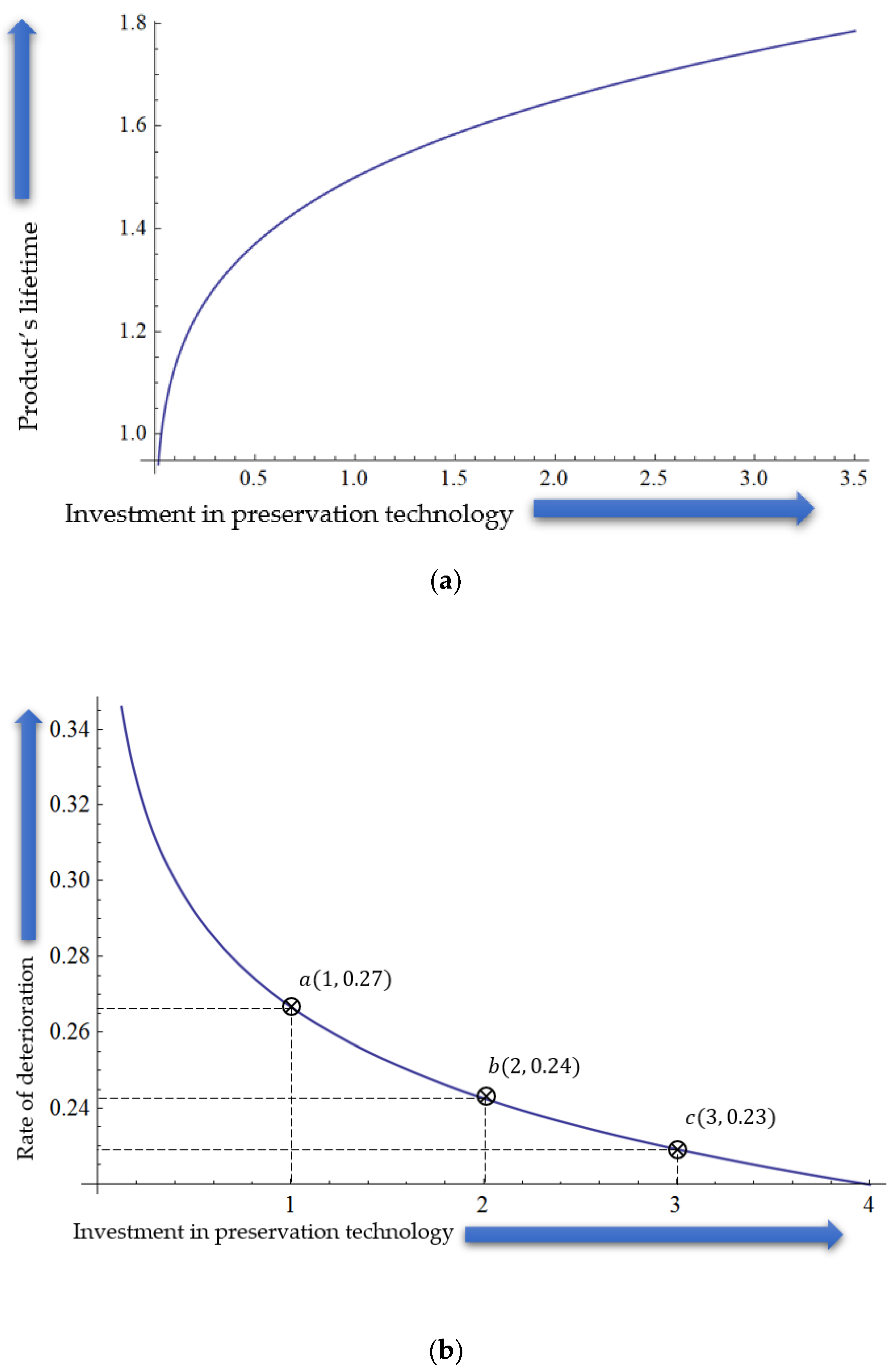
• How does the preservation effect quantitatively the lifetime/deterioration/freshness of a fresh food product?
• What is the effect of SSMD policy on lot size and replenishment cycle?
• How do the preservation and SSMD policies affect total supply chain profit?

Besides, unlike the assumptions of Ben–Daya et al. [11] and Cárdenas–Barrón [12], the ordering cost and inventory holding cost at each retailer cannot be the same due to several factors related to the inventory management system. Therefore, this research considers unequal ordering costs, inventory holding costs, and replenishment quantities for all the retailers in a multi-retailer two-echelon supply chain system. Further, unlike several authors who proposed an unchanged effect of preservation with time, this research suggests that the effect of preservation decreases with time.

2. Literature Review

The literature review is classified into the following domains and the research gap is concluded after investigating these literature domains.

2.1. Single Setup Multiple Deliveries (SSMD)

In the literature, several authors discussed supply chain models considering single-setup multiple deliveries (SSMD) policies involving multiple retailers in a coordinated supply chain system. SSMD policy was introduced by Goyal [13], who considered multiple shipments/deliveries in a two-tier supply chain system with a single manufacturer and single retailer. He extended the famous model of Banerjee [14], who considered lot-for-lot model between a manufacturer and a retailer. Later, Lu [15] discussed a supply chain system involving single-vendor and multiple retailers by considering single shipment to all the retailers, and Goyal [16] extended the model of Lu [15] by adding geometrically increasing shipment size for the next deliveries. The state-of-the-art research on SSMD was summed up by Thomas and Griffin [17], who provided a comprehensive literature review for the supply chain models considering multiple retailers’ systems adopting a coordinated approach. Research continued in this important domain and Hill [18] improved the models by considering an increase in lot size by a fixed factor. Hill [19] also designed an algorithm to solve SSMD models for globally optimal solutions.

Goyal and Nebebe [20] added to the literature by considering different lot sizes for the first shipment while considering equal lot sizes for the each following shipment within an SSMD setup. A collaborative SSMD policy for deteriorating products was proposed by Yang and Wee [21] to prove that the cost was reduced significantly by adopting an integrated/collaborative policy. Later, Khouja [22] extended the collaborative SSMD policy by considering equal cycle times at all stages. Similarly, Wang and Sarker [23] introduced an assembly-type Kanban system considering SSMD policy to prove that coordination mechanisms among the supply chain players are more beneficial. Likewise, Siajadi et al. [24] suggested that a collaborative strategy between supply chain players is more profitable when considering SSMD policy. The SSMD policy was further adopted by Chan and Kingsman [25] in a coordinated two-echelon supply chain system, where the cycle time of the buyer is synchronized with that of the manufacturer. They proved that the supply chain works better when these cycle times are in a synchronized pattern. Cárdenas–Barrón [12] improved the model of Khouja [22] by considering multiple (more than three)-stage supply chains involving multiple manufacturers, multiple assemblers, and multiple retailers. Ben–Daya and Al-Nassar [26] extended the idea of Lu [15], assuming that shipments/deliveries for retailers are prepared while the production process is running, considering the cycle time of each stage as an integer multiplier of the cycle time of the adjacent downstream stage.

The research in the same field was continued by Darwish and Odah [27], who considered a two-echelon, vendor–buyer supply chain system, where the vendor manages inventories (VMI) of multiple retailers within contractual specified bounds and is liable to pay a penalty when inventory exceeds or falls short of the specified boundaries, considering equal cycle time of all the retailers and capacity constraints. Roy et al. [28] proposed an inventory model for imperfect quality, deteriorating products with equal lengths of replenishment periods of each shipment, and allowing partially backlogged shortages at the end of the planning period that were caused by capacity constraints. Ben–Daya et al. [11] considered a vertically integrated, three-echelon supply chain system with a single supplier, single manufacturer, and multiple retailers, allowing multiple shipments to the retailers within a single cycle of the manufacturer. They obtained a near-optimal solution of the model by using the derivative-free solution approach. Sajadieh et al. [29] modeled a three-echelon supply chain system involving multiple suppliers, multiple manufacturers, and multiple retailers, considering a stochastic lead time of delivery from manufacturers to the retailers.

This dimension was further explored by Yang et al. [3], who proposed a closed-loop supply chain system considering single manufacturers and multiple retailers and adopting the SSMD policy for deteriorating products, the demand of which was price-sensitive. Sana et al. [30] suggested a three-echelon supply chain model of multi-items involving multiple suppliers, multiple manufacturers, and multiple retailers, considering multiple shipments to the retailers for imperfect quality items at each tier of the supply chain that were sent back to the upstream player of the supply chain at a lower price. They proved that a collaborative system is more favorable as compared to the Stackelberg game structure. A three-echelon supply chain system was further investigated by Yang et al. [31] by considering multiple suppliers, single manufacturers, and multiple retailers, and assuming multiple deliveries to the retailers. Later, Jia et al. [32] improved the literature by considering the shortest shipment cycle within the SSMD setup to improve the performance of the system. Considering a deteriorating product, Azadi et al. [6] suggested that the shipment cycle is an important variable with the SSMD setup that helps reducing waste by curtailing deterioration. Similarly, Sarkar et al. [8] considered the SSMD policy to integrate the replenishment cycle with the setup time, production time, and transportation time. Similarly, Song et al. [33] suggested that the multi/omni-channel retailing is optimal for fresh food products. Considering the discussed theories, this study adopts an SSMD policy in a two-echelon supply chain system considering single manufacturers and multiple retailers and considering unequal lot sizes at each retailer.

2.2. Product Deterioration

Deterioration is commonly realized as the spoilage of the products when they are stored in infeasible conditions. However, a broader definition of deterioration refers to its decreased consumable quantity or decreased market value that can be due to its spoilage, evaporation, leakage, outdated model, etc. Several researchers investigated the deteriorating inventory models and provided optimal solutions. The rate of deterioration has been modeled in several ways. Among the pioneer attempts of studying deteriorating inventories is the work of Ghare and Schrader [34] and Sachan [35]. They proposed inventory models by considering constant deterioration. Later, Chang and Dye [36] introduced partial backlogging in an inventory model by considering a constant deterioration rate.

The assumption of a constant rate of deterioration was relaxed by Skouri et al. [37] by considering the time-varying deterioration. Shah et al. [38] suggested that the deterioration of the products starts after a specific time interval when these products are stored as an inventory and considered the variable rate of deterioration. Wu et al. [39] considered the variable rate of deterioration and proposed the idea of expiration time at which a product completely deteriorates. Qin et al. [40] suggested that the rate of deterioration increases with temperature as well as time. Iqbal and Sarkar [41] and Iqbal and Sarkar [42] suggested that the rate deterioration depends on the products’ lifetime which is controllable.

The idea of a maximum lifetime-dependent deterioration rate was incorporated in the research of Chen and Teng [43], Wang et al. [44], Wu et al. [39], and Shah et al. [45]. Feng et al. [46] considered that the freshness of perishable products depends on the time and maximum lifetime of the products, which is related to the rate of deterioration. Likewise, Chen et al. [47] proposed the quality-based shipment consolidation policy for deteriorating products considering preservation. The effect of transportation and deterioration on the environment was studied and carbon emissions were calculated by Daryanto et al. [48]. Iqbal et al. [49] proposed an idea of the rate of deterioration that depends on the vulnerability of a product with respect to its environment. Considering various ideas from the literature, this study proposes that the deterioration rate has a direct relationship with the vulnerability to deterioration of a specific product, and that the deterioration rate is a function of a product’s lifetime.

2.3. Preservation Policies

The most used method to avoid losses done by deterioration of food products is preservation. Preservation is of two types: preservatives and storage conditions. Preservation conditions comprise temperature, humidity, aeration, sanitation, etc., which help to reduce the rate of deterioration by diminishing the activities of the microbe causing spoilage of the products. The effect of preservation technology on the rate of deterioration has been discussed by several researchers. Hsu et al. [50] suggested that deterioration decreases linearly with preservation investment. The same idea was adopted by Dye [51], who informed that the deterioration rate decreases linearly with preservation investment. He and Huang [52] proposed that the deterioration rate is an exponential function of preservation investment, inversely. Yang et al. [53] followed the idea that preservation investment reduces the deterioration rate linearly.

Unlike previous citations, Shah et al. [45] suggested that a reduced deterioration rate depends on preservation investment. Tsao [54] considered a novel idea of preservation efforts and proposed that deterioration decreases quadratically related to the preservation investment. Dye and Yang [55] considered a two-echelon supply chain system with SSMD policy for perishable products. They suggested that the deterioration rate decreases linearly with the preservation investment. Giri et al. [56] and Mishra et al. [57] suggested that the rate of deterioration decreases linearly with investment in preservation technology. Khakzad and Gholamian [58] concluded that a greater number of inspection periods decrease the average rate of deterioration. Having a critical look on the literature, it is observed that, while proposing linear, quadratic, and exponential relations between preservation investment and reduction in deterioration rate, the authors overlooked the fact that preservation technology can minimize deterioration to a specific level. In practical scenarios, the magnitude of decrease in the rate of deterioration reduces for an additional preservation investment. An additional preservation investment beyond an optimal point merely increases the cost, while the reduction in deterioration is negligible. Therefore, this research provides the policy of preservation investment in way that the magnitude of decrease in the rate of deterioration reduces with an additional preservation investment. This policy is abbreviated as the MDRDRMIP policy. Table 1 exhibits the share of this study to the literature. The term “conventional” in this table reflects that by applying preservation, the reduction in the rate of deterioration remains the same with the passage of time.

Table 1. Literature enrichment by this study.

Authors	Two-Echelon SCM	Multiple Retailers	Unequal Lot Size	SSMD	Preservation Policy
Goyal [13]	✓			✓
Lu [15]	✓	✓
Goyal [16]	✓	✓	✓	✓
Hill [18]	✓		✓	✓
Goyal and Nebebe [20]	✓		✓	✓
Woo et al. [59]	✓	✓
Yang and Wee [21]	✓	✓
Khouja [22]		✓		✓
Wang and Sarker [23]				✓
Siajadi et al. [24]	✓	✓		✓
Chan and Kingsman [25]	✓	✓		✓
Ertogral et al. [60]	✓			✓
Ben-Daya and Al-Nassar [26]		✓	✓	✓
Darwish and Odah [27]	✓	✓		✓
Hsu et al. [50]					Conventional
Ben-Daya et al. [11]		✓		✓
Dye [51]					Conventional
Sana et al. [30]		✓		✓
Yang et al. [53]					Conventional
Yang et al. [31]		✓		✓
Jia et al. [32]		✓
Dye and Yang [55]	✓			✓	Conventional
Giri et al. [56]	✓				Conventional
Azadi et al. [6]	✓	✓		✓
Sarkar et al. [8]	✓	✓		✓
This paper	✓	✓	✓	✓	MDRDRMIP

Table 1. Literature enrichment by this study.

Authors	Two-Echelon SCM	Multiple Retailers	Unequal Lot Size	SSMD	Preservation Policy
Goyal [13]	✓			✓
Lu [15]	✓	✓
Goyal [16]	✓	✓	✓	✓
Hill [18]	✓		✓	✓
Goyal and Nebebe [20]	✓		✓	✓
Woo et al. [59]	✓	✓
Yang and Wee [21]	✓	✓
Khouja [22]		✓		✓
Wang and Sarker [23]				✓
Siajadi et al. [24]	✓	✓		✓
Chan and Kingsman [25]	✓	✓		✓
Ertogral et al. [60]	✓			✓
Ben-Daya and Al-Nassar [26]		✓	✓	✓
Darwish and Odah [27]	✓	✓		✓
Hsu et al. [50]					Conventional
Ben-Daya et al. [11]		✓		✓
Dye [51]					Conventional
Sana et al. [30]		✓		✓
Yang et al. [53]					Conventional
Yang et al. [31]		✓		✓
Jia et al. [32]		✓
Dye and Yang [55]	✓			✓	Conventional
Giri et al. [56]	✓				Conventional
Azadi et al. [6]	✓	✓		✓
Sarkar et al. [8]	✓	✓		✓
This paper	✓	✓	✓	✓	MDRDRMIP

Keeping in view the above discussion, this study defines policies for a two-echelon supply chain system involving a single manufacturer and multiple retailers, where the retailers’ demand is fulfilled in multiple shipments. The replenishment cycle at all the retailers is same, whereas the lot size at each retailer is different. The products under consideration are deteriorating in nature. Therefore, the MDRDRMIP policy is introduced to control the rate of deterioration in a realistic situation as compared to Hsu et al. [50] and Dye and Yang [55]. Finally, profit per unit time of the centralized/coordinated supply chain is maximized by obtaining optimal values of the retailers’ replenishment cycle, number of deliveries/shipments to retailers by manufacturer in its cycle, and preservation investment. This study is structured as follows: Section 3 defines the research problem and model assumptions. Section 4 provides the mathematical model and explains the solution procedure. Section 5 validates the provided mathematical model with the help of numerical experiments and demonstrates important results through graphical illustrations. Section 6 exhibits imperative managerial insights related the provided models and results. Section 7 summarizes the study by concluding from the proposed model and experiments and provides future extensions of this research.

3. Problem Definition, Notation and Assumptions

The considered research problem is comprehensively defined in this section with useful assumptions. The notation to explain the mathematical models is also exhibited in this section.

3.1. Problem Definition

This study investigates a supply chain comprising of a single manufacturer and $n$ number of retailers considering deteriorating products. The manufacturer produces and delivers products to retailers in multiple deliveries. The transportation cost is considered within the setup cost of the manufacturer. Other costs at the manufacturer level include the cost of material, production, and inventory stock. In a real-world situation, retailers of a particular product are located at different regions geographically and demographically. They receive the products from the manufacturer as per the scheduled replenishment period shared by all the retailers. The demand at each retailer is different due to several factors related to the region, population, advertisement, etc. Therefore, each retailer receives different lot sizes from manufacturer depending on their demands.

The products under consideration are deteriorating in nature and they start deteriorating when delivered to retailers. In order to minimize the effects of deterioration, several preservation techniques are used in form of cold storage, humidity, sanitation, etc. Preservation reduces the rate of deterioration, yet some products deteriorate during the cycle. Therefore, retailers demand from the manufacturer the amount of the product which fulfills customers’ demand and compensates the deteriorated quantity during the retailers’ cycle. Thus, the manufacturer’s demand is the sum of the demand of $n$ number of retailers and the anticipated deteriorated quantity at all the retailers. The manufacturer purchases the raw material and produces exactly the same number of items as are demanded by all the retailers, thus creating no shortages. The manufacturer plans its production in a way that the rate of production depends on the rate of demand. As the rate of demand remains constant, therefore the rate of production also remains constant during the cycle. The manufacturer supplies the finished products to $n$ number of retailers in $m$ number of deliveries. Therefore, the manufacturer’s production time is $m$ times the joint cycle time $T$ of the retailers. The ordering cost and inventory holding cost at each retailer is different due to the difference in their location, salary structures, management system, etc. Other costs at the retailers include the purchasing cost and cost of preservation investment. The system is considered as a centralized supply chain, and therefore, the purchasing cost of retailer is the same as the manufacturer’s selling price. The selling price of each retailer is different due to different cost structures at each retailer. Figure 1 illustrates the configuration of the supply chain system under consideration.

3.2. Assumptions

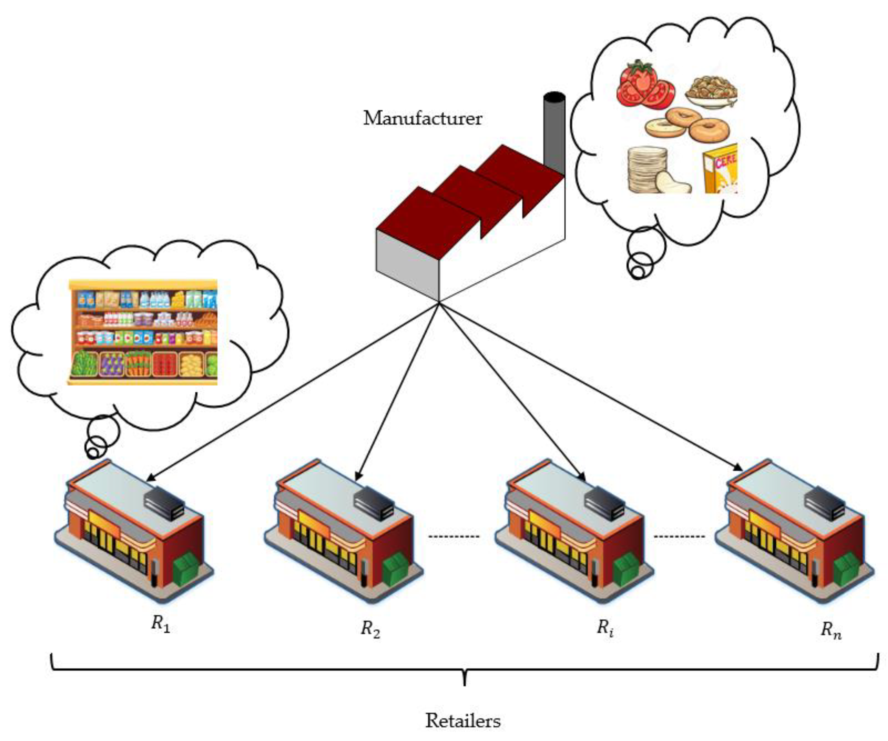
• A single manufacturer supplies fresh products to the multi-retailers to constitute a supply chain system.
• The manufacturer supplies the produced items to retailers in multiple deliveries, which is known as a single setup multi-delivery (SSMD) policy. Therefore, the cycle time of the manufacturer is the integer multiple of the retailers’ cycle time. This integer is the number of deliveries/shipments to the retailers per cycle of the manufacturer.
• Shipments/deliveries for retailers are prepared from a production batch while the production is continued [26].
• The cycle time of all the retailers is equal, i.e., the inventory is replenished at all the retailers at the same point of time [11].
• The customer demand at all the retailers is known, constant, and different.
• As the demand at each retailer is different, therefore, this model assumes an unequal lot size for each retailer.
• The ordering cost and cost of inventory carrying are different for each retailer.
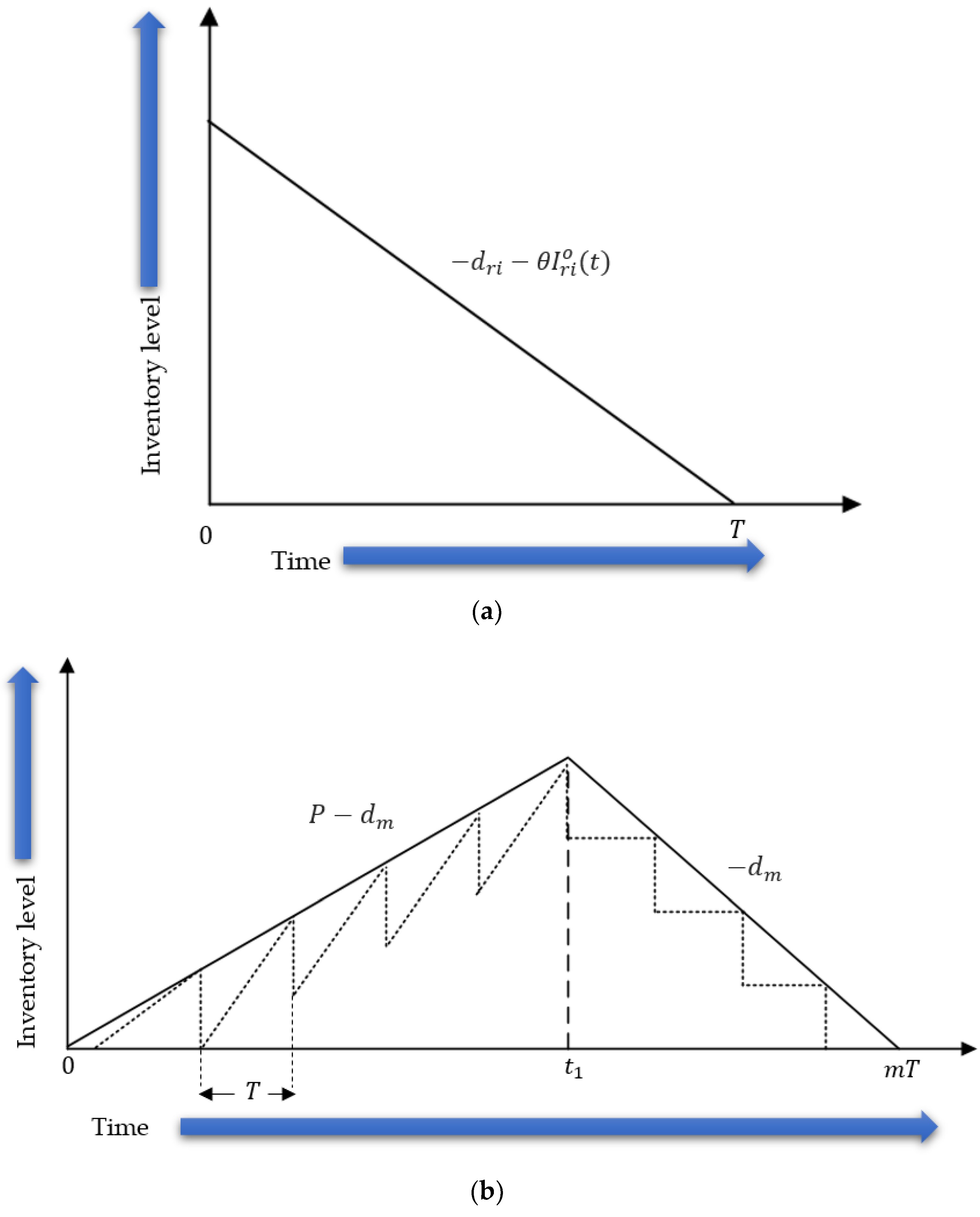
• The products under consideration are deteriorating in nature, and deteriorate at a constant rate. Practically, the products start deteriorating after being replenished at the retailer. This study includes this fact by considering no deterioration at the manufacturer.
• The rate of deterioration is curtailed using preservation technology. The magnitude of decrease in deterioration decreases with the additional preservation investment, as is explained in Section 4 and demonstrated by Equation (1) and Figure 2b.
• The rate of production depends on the demand rate [40], i.e., assuming where the production rate and the demand rate at the manufacturer are.
• The inventory holding cost at the manufacturer is less than the inventory holding cost at the retailers, i.e.
• There are no shortages, i.e., all the customers are satisfied to fulfill their demand.
• The supply chain is vertically integrated, such that the optimal value of profit is obtained as a centralized system.

4. Model Formulation and Solution

This is a natural phenomenon that the products with longer lifetimes deteriorate at slower rates. For example, the rate of deterioration of harvested grains is less as compared to the rate of the deterioration of fruits and vegetables. Therefore, this study assumes that the lifetime of a product governs its rate of deterioration. In a comparison with different types of products, the longer the lifetime of a product, the shorter its rate of deterioration will be.

Hence:

$$\theta =\frac{\alpha }{L}, \alpha \le L,$$

where $\alpha$ is the degree of vulnerability of a product to deterioration, which depends on the type of product and the ambient conditions where the product is stored. The greater the value of $\alpha$, the more likely it is vulnerable to deterioration. For some products, the value of $\alpha$ is close to zero, which means those products do not deteriorate. For example, the value of $\alpha$ approaches zero for vinegar and chocolate syrup. Therefore, they do not deteriorate quickly in normal circumstances. In contrast, the value of $\alpha$ is high for ice cream without cold storage.

Preservation increases the lifetime of the products. The quality of preservation technology is increased by investing more in this technology. However, practically, this increase in investment increases the lifetime and decreases the deterioration rate to a specific level. By investing in preservation technology beyond that level, the increase in lifetime and decrease in deterioration is practically negligible. Therefore, the preservation investment is modeled in such a way that increases the lifetime, while the magnitude of increase decreases with greater preservation investment. This fact is exhibited mathematically in the below equation.

$$\widehat{L}=\left(1+x{p}^{\gamma }\right)L; \gamma <1$$

The same fact is illustrated in Figure 2a. We considered a product assuming these parameters $\alpha =0.4, x=2, \gamma =0.2, L=0.5$, and plotted a graph for the product’s lifetime $\widehat{L}$ against different values of preservation investment p.

The value of $x$ is the degree of effectiveness of preservation cost on the lifetime of the products. The value of $x$ depends on the right choice of preservation conditions for a specific product.

The intensity of the deterioration changes with a product’s lifetime which is a function of preservation. The decreased deterioration rate is exhibited below.

$$\widehat{\theta }=\frac{\alpha }{\left(1+x{p}^{\gamma }\right)L}$$

(1)

The value of $\gamma$ is proposed to be less than one to represent the effect of preservation on lifetime and deterioration in a real-world situation. In contrast to many researchers, who proposed the effect of preservation investment on the deterioration in a conventional way, this study proposes that the magnitude of the decrease in deterioration keeps decreasing with additional preservation investment, and after a specific amount of investment, the decrease in deterioration will be negligible, no matter how much preservation cost is invested. This is illustrated in the Figure 2b. We considered the same product assuming the same parameters as we assumed for lifetime graph, i.e., $\alpha =0.4, x=2, \gamma =0.2, L=0.5$, and plot a graph for rate of deterioration $\widehat{\theta }$ against different values of preservation investment p.

Figure 2b shows that, for the first unit of preservation investment, the rate of decrease in deterioration is $\frac{0.8-0.27}{1-0}=0.53$, for the second unit of preservation investment the rate of decrease in deterioration is $\frac{0.27-0.24}{2-1}=0.03$, and for the third unit of preservation investment the decrease in deterioration is $\frac{0.24-0.23}{3-2}=0.01$. Therefore, the suggested formula for the rate of deterioration with effects of preservation investment is closer to the real-world situations, as the magnitude of the decrease in deterioration decreases with additional preservation investment.

4.1. Retailers’ Model

The proposed system considers $n$ number of retailers, who receive the finished products from a common manufacturer. The rate of demand at retailer $i$ is $d_{ri}$. As the products under consideration are deteriorating in nature, which deteriorate at a constant rate $\widehat{\theta }$, therefore, a fraction of the retailer’s inventory deteriorates during the retailers’ inventory cycle. The inventory of the products at a retailer depletes due to the cumulative effect of demand and deterioration. The behavior of the inventory level for retailer $i$ for one cycle is illustrated in Figure 3a. The stock is fully exhausted at the end of planning horizon at time $T$ and next delivery is received.

The governing differential equation for the inventory at retailer $i$ is as given below, which shows that the rate of change of inventory from $0$ to $T$ is the negative rate of demand and deterioration, as the items are taken out of inventory.

$$\frac{d{I}_{ri}^o\left(t\right)}{dt}=-d_{ri}-\widehat{\theta }{I}_{ri}^o, 0\le t\le T$$

The above expression is the slope of the function of on-hand inventory at retailer i.

The value of the function $I_{ri}^o\left(t\right)$, at any time $t$, is calculated from the given slope by using the inventory condition $I_{ri}^o\left(t\right)=0$ at $t=T$, as:

$$I_{ri}^o\left(t\right)=\frac{d_{ri}}{\widehat{\theta }}\left(e^{\widehat{\theta }\left(T-t\right)}-1\right), 0\le t\le T$$

The common operations at a retailer, which incur some cost, comprise ordering and purchasing the products from the manufacturer, and carrying out the inventory of those products. A special operation for the deteriorating products under consideration is maintaining the preservation conditions. Several costs, which are considered at the retailers’ level, are explained, and calculated below.

4.1.1. Ordering Cost

There are several activities, which are performed while ordering and receiving a replenishment lot by a retailer from the manufacturer, such as the preparation of purchase orders, transportation, receiving, inspection, handling the products and placing them in storage, and auditing, etc. The costs incurred to perform these activities are cumulatively termed as the ordering costs, which is considered per order of the product. As this study considers a single cycle of retailer $i$, therefore, ordering cost per cycle at retailer $i$ is given as in the below equation.

$$\mathrm{Ordering} \mathrm{cost} \mathrm{per} \mathrm{cycle}=A_{ri}$$

4.1.2. Purchasing Cost

The retailers purchase at a fixed cost per unit, which satisfies the customer demand during the complete cycle. The cost of acquisition of one unit of the product by the $i–th$ retailer is the purchasing cost per unit $P{C}_{ri}$, which is used to compute the purchasing cost per cycle. The stock of the product at a retailer does not deplete only due to the customer demand, but also due to the effects of deterioration. Therefore, a retailer orders/purchases the amount of the product that fulfills the customer demand during the complete cycle by recompensing the effects of deterioration. Thus, the ordering/purchasing quantity per cycle of retailer $i$ is the sum of customer demand per cycle and the number of items that would deteriorate in a cycle. The demand per cycle of retailer i is calculated below.

$$D_{ri}={\displaystyle \underset{0}{\overset{T}{\int }}{d}_{ri}dt}=d_{ri}T$$

Similarly, the number of items that deteriorate at retailer $i$ during one cycle are computed as below.

$$N_{di}=\widehat{\theta }{\displaystyle \underset{0}{\overset{T}{\int }}{I}_{ri}^o\left(t\right)dt}=\frac{d_{ri}}{\widehat{\theta }}\left(e^{\widehat{\theta }T}-\widehat{\theta }T-1\right)$$

The retailer $i$ will purchase an amount from the manufacturer that will fulfill the customer’s demand and will also compensate for the losses due to deterioration, such that there will be no shortages. Therefore, the purchasing quantity of the retailer $i$ is as given below.

$$P{Q}_{ri}=D_{ri}+N_{di}$$

(2)

Thus, the purchasing cost of the product per cycle for retailer $i$ is calculated and expressed in the following equation.

$$\mathrm{Purchasing} \mathrm{cost} \mathrm{per} \mathrm{cycle}=P{C}_{ri}P{Q}_{ri}$$

4.1.3. Inventory Holding Cost

The retailers carry stock of the products to fulfill the demand of their customers during the planning horizon. Storing the products as inventory incurs some costs, such as rent of the storage place, temperature balance, lighting, record keeping, taxes, etc., the cumulation of which is termed as the inventory holding cost. For the retailer $i$, $h_{ri}$ is the cost of holding one unit of the product per unit time.

The stock of inventory that is carried by the retailer $i$ during one cycle $\left[0,T\right]$, on which the inventory holding cost is considered, is calculated, and expressed in the below equation.

$$I_{ri}=\underset{0}{\overset{T}{\int }}{I}_{ri}^o\left(t\right)dt=\frac{d_{ri}}{{\widehat{\theta }}^2}\left(e^{\widehat{\theta }T}-\widehat{\theta }T-1\right)$$

Using the above expression, the cost of the inventory carrying per cycle of retailer $i$ is provided as following.

$$\mathrm{Inventory} \mathrm{holding} \mathrm{cost} \mathrm{per} \mathrm{cycle}=h_{ri}{I}_{ri}$$

4.1.4. Preservation Cost

At a retailer, the rate of deterioration is curtailed by applying special inventory conditions that are called the preservation conditions. The requirement of preservation conditions depends on the type of the product. The most used preservation conditions include cold storage, air velocity, relative humidity, atmospheric composition, and sanitation. The cost of preservation $p$ per unit per unit time is the cost expended to maintain the optimum level of such conditions, which reduce the deterioration rate by increasing lifetime of the products. The cost of preservation per cycle at retailer $i$ is calculated in the equation as below.

$$\mathrm{Cost} \mathrm{of} \mathrm{preservation} \mathrm{per} \mathrm{cycle}=p{I}_{ri}$$

4.1.5. Total Cost per Unit Time

The total cost at retailer $i$ is the sum of its ordering cost, purchasing cost, inventory holding cost, and preservation cost, which is given per unit time in the below equation.

$$\mathrm{Total} \mathrm{cost} \left(T{C}_{ri}\right)=\frac{1}{T}\left(A_{ri}+P{C}_{ri}P{Q}_{ri}+h_{ri}{I}_{ri}+p{I}_{ri}\right)$$

4.1.6. Sales Revenue per Unit Time

A retailer sells its product at a fixed selling price per unit $S{P}_{ri}$. The selling price at each retailer is considered as different due to their different setup, cost structure, and location, which causes varied costs for each retailer. The sales revenue of the retailer $i$ per unit time is expressed in the below equation.

$$S{R}_{ri}=S{P}_{ri}{d}_{ri}$$

4.1.7. Retailers’ Profit per Unit Time

A retailer earns profit by selling its products during the planning horizon. The profit of the retailer $i$ is given below.

$$T{P}_{ri}=S{R}_{ri}-T{C}_{ri}$$

The total profit per unit time of $n$ retailers is calculated as below.

$$T{P}_r={\displaystyle \sum _{i=1}^n\left(S{R}_{ri}-T{C}_{ri}\right)}$$

(3)

4.2. Manufacturer’s Model

The manufacturer plans its activities to produce the products after the retailers order their purchase quantity. It produces exactly that amount of the product, which is demanded by all the retailers. Thus, the demand that the manufacturer faces for one cycle of retailers is the sum of demands of all the retailers. Therefore, the manufacturer’s demand per retailers’ cycle is given below.

$$\mathrm{Manufacturer}’\mathrm{s} \mathrm{demand} \mathrm{per} \mathrm{retailers}’ \mathrm{cycle}={\displaystyle \sum _{i=1}^{n}P{Q}_{ri}}={\displaystyle \sum _{i=1}^n\left(D_{ri}+N_{di}\right)}$$

This model assumes that there are $m$ number of deliveries/shipments to the retailers per the manufacturer’s cycle, and therefore the manufacturer’s demand per cycle is $m$ times the retailers’ purchase quantity per cycle that is provided as follows.

$$D_m=m{\displaystyle \sum _{i=1}^n\left(D_{ri}+N_{di}\right)}$$

Similarly, the manufacturer’s cycle time is $m$ times the cycle time of a retailer. Thus, $mT$ is the cycle time of the manufacturer. By using the demand per manufacturer’s cycle and its cycle time, the rate of demand per unit time at the manufacturer is calculated and exhibited as given below.

$$d_m=\frac{D_m}{mT}=\frac{{\displaystyle \sum _{i=1}^n\left(D_{ri}+N_{di}\right)}}{T}$$

The manufacturer produces the products as per demand and the production rate is proportional to the demand rate, which is given below.

$$P=k{d}_m=\frac{k{\displaystyle \sum _{i=1}^n\left(D_{ri}+N_{di}\right)}}{T}$$

There are no shortages, and the production rate is always higher than the demand rate, i.e., $k>1$. The manufacturer plans its schedule in a way such that production is run from $0$ to $t_1$ and retailers’ orders are fulfilled during the complete manufacturing cycle from $0$ to $mT$ in multiple shipments/deliveries $m$. In order to simplify the calculations, this study considers a continuous flow system as is modeled by Yang et al. [3]. From $0$ to $t_1$ the rate of inventory replenishment is $P-d_m$, while from $t_1$ to $mT$, the rate of inventory depletion is $-d_m$. The inventory level rises while the production cycle is continuing, and it begins to deplete at time $t_1$ when production is completed. The inventory stock is completely depleted at the end of the planning horizon at time $mT$, as shown in Figure 3b.

The differential equations governing the inventory level at the manufacturer are expressed below. Equation (4) shows the combined effect of the rate of production and demand during the interval $\left(0,t_1\right)$. The cumulative effect of production and demand on the rate of change in inventory level is positive because the production rate is higher as compared to the rate of demand. Therefore, the inventory stock is replenished during production time. The inventory stock starts depleting when the production time is over. Equation (5) depicts the effect of the demand on the rate of change in the inventory level during the interval (t₁, mT).

$$\frac{d{I}_m^a\left(t\right)}{dt}=P-d_m=\left(k-1\right)d_m, 0\le t\le t_1$$

(4)

$$\frac{d{I}_m^b\left(t\right)}{dt}=-d_m, t_1\le t\le mT$$

(5)

Equations (4) and (5) calculate the slope of the functions of the on-hand inventory at the manufacturer during the intervals $\left(0,t_1\right)$ and $\left(t_1,mT\right)$, respectively. The value of the functions $I_m^a\left(t\right)$ and $I_m^b\left(t\right)$ is calculated by using the below inventory conditions.

$$\begin{array}{l}{I}_m^a\left(t\right)=0 \mathrm{at} t=0\\ I_m^b\left(t\right)=0 \mathrm{at} t=mT\end{array}$$

$$I_m^a\left(t\right)=\left(k-1\right)d_{m}t, 0\le t\le t_1$$

$$I_m^b\left(t\right)=d_m\left(mT-t\right), t_1\le t\le mT$$

From Figure 4, it can be observed that, for an instant, the level of inventory for both the intervals is the same when $t=t_1$. Therefore:

$$\begin{array}{l}\left(k-1\right)d_m{t}_1=d_m\left(mT-t_1\right)\\ \Rightarrow \hspace{1em}\hspace{1em}\hspace{1em}{t}_1=\frac{mT}{k}\end{array}$$

Thus, $t_1$ is a dependent variable, the value of which is decided by the values of the retailers’ cycle time $T$, number of deliveries/shipments $m$ to retailers, and the constant for the rate of production k.

The usual operations, which are carried out at the manufacturer and which incur some cost include the purchasing of raw material, production setup, manufacturing/production process, and inventory of the finished products. Several costs which are considered by manufacturer are explained and calculated below.

4.2.1. Setup Cost

The activities, such as the preparation of production machines, supply of raw materials, and arrangement of storing finished products, are related to the production setup activities. The cost incurred to perform these activities is termed as the production setup cost. The production setup cost per cycle of the manufacturer is exhibited as follows.

$$\mathrm{Setup} \mathrm{cost} \mathrm{per} \mathrm{manufacturer}’\mathrm{s} \mathrm{cycle}=C_{set}$$

4.2.2. Material Purchasing Cost

In the manufacturing industry, usually the cost of materials is the highest among other costs. The selection of qualitative raw material is important to produce a product of the required quality. The requirement of materials depends on the type of product. For some products only one type of raw material is used, while for other products more than one type of raw material is used. The cost incurred by all types of materials that are used to produce one unit of the product is designated as the material cost per unit $C_{mt}$. As the production system is assumed to be perfect, therefore, the material is purchased as per production quantity. The production quantity produced per manufacturer’s cycle is expressed in Equation (6). The total material cost per manufacturer’s cycle is expressed below.

$$\mathrm{Material} \mathrm{purchasing} \mathrm{cost} \mathrm{per} \mathrm{manufacturer}’\mathrm{s} \mathrm{cycle}=C_{mt}{N}_p$$

where $N_p$ is the number of items produced per manufacturer’s cycle and is expressed below.

$$N_p={\displaystyle \underset{0}{\overset{t_1}{\int }}Pdt=m{\displaystyle \sum _{i=1}^n\left(D_{ri}+N_{di}\right)}}$$

(6)

4.2.3. Production Cost

The production process is the value addition phase within a supply chain, which converts the raw material into finished products through available resources. Several operations are involved in the production process, which acquires some costs, including labor cost, cost of maintenance, utility costs, etc., the cumulation of which is named the production cost. The production cost is considered per unit of the produced items, as $C_p$. The production cost per manufacturer’s cycle is computed as given below.

$$\mathrm{Production} \mathrm{cost} \mathrm{per} \mathrm{manufacturer}’\mathrm{s} \mathrm{cycle}=C_p{N}_p,$$

where $N_p$ is the number of items produced per cycle, as provided in Equation (6).

4.2.4. Inventory Holding Cost

The produced items at the manufacturer are stored as the inventory, which fulfills the demand of the retailers. As a greater number of items are produced as compared to those demanded during the production cycle, the inventory level thus increases during production time and gradually decreases when production is stopped, until it completely depletes at the end of the manufacturer’s cycle. The manufacturer’s held inventory per cycle $\left(I_m\right)$, which incurs inventory holding cost, is given below.

$$I_m={\displaystyle \underset{0}{\overset{t_1}{\int }}{I}_m^a\left(t\right)}dt+{\displaystyle \underset{t_1}{\overset{mT}{\int }}{I}_m^b\left(t\right)}dt=\frac{d_m}{2}\left(\frac{k-1}{k}{\left(mT\right)}^2\right)$$

The total inventory holding cost per manufacturer’s cycle is provided below.

$$\mathrm{Inventory} \mathrm{holding} \mathrm{cost} \mathrm{per} \mathrm{manufacturer}’\mathrm{s} \mathrm{cycle}=h_m{I}_m$$

4.2.5. Total Cost per Unit Time

The total cost at the manufacturer is the aggregate of setup cost, material cost, production cost, and inventory holding cost, as is provided in the following equation.

$$\mathrm{Manufacturer}’\mathrm{s} \mathrm{total} \mathrm{cost} \mathrm{per} \mathrm{unit} \mathrm{time} \left(T{C}_m\right)=\frac{1}{mT}\left(C_{set}+C_{mt}{N}_p+C_p{N}_p+h_m{I}_m\right)$$

4.2.6. Sales Revenue per Unit Time

The manufacturer’s sale per unit time is $d_m$ units which are sold at a price $S{P}_m$ per unit. The manufacturer’s revenue per unit time is calculated as follows.

$$S{R}_m=S{P}_m{d}_m$$

As the manufacturer sells its product to the retailers, the selling price of manufacture is the same as the purchasing cost of the retailers. Therefore,

$$S{P}_m=P{C}_{ri}.$$

4.2.7. Manufacturer’s Profit per Unit Time

The total profit per unit time of manufacturer $T{P}_m$ is expressed below which is calculated by using the value of the revenue and cost.

$$T{P}_m=S{R}_m-T{C}_m$$

(7)

4.2.8. Total Profit per Unit Time of the Supply Chain

The supply chain’s total profit per unit time $TP$ in a centralized system is computed by adding the profit per unit time of all the retailers $T{P}_r$ and that of the manufacturer $T{P}_m$. Adding Equations (3) and (7), and simplifying the results, the total profit per unit of time is obtained as follows.

$$TP\left(m,p,T\right)=T{P}_r+T{P}_m={\displaystyle \sum _{i=1}^n\left\{S{R}_{ri}-\frac{1}{T}\left(A_{ri}+h_{ri}{I}_{ri}+p{I}_{ri}\right)\right\}}-\frac{1}{mT}\left(C_{set}+C_{mt}{N}_p+C_p{N}_p+h_m{I}_m\right)$$

$$\begin{array}{l}={\displaystyle \sum _{i=1}^n\left[S{P}_{ri}{d}_{ri}-\frac{1}{T}\left\{A_{ri}+\left(h_{ri}+p\right)d_{ri}{\left(\frac{\left(1+x{p}^{\gamma }\right)L}{\alpha }\right)}^2\left(e^{\frac{\alpha T}{\left(1+x{p}^{\gamma }\right)L}}-\frac{\alpha T}{\left(1+x{p}^{\gamma }\right)L}-1\right)\right\}\right]}\\ -\frac{1}{mT}\left[\begin{array}{l}{C}_{set}+\left(C_{mt}+C_p\right)m{\displaystyle \sum _{i=1}^n\left\{d_{ri}T+d_{ri}\frac{\left(1+x{p}^{\gamma }\right)L}{\alpha }\left(e^{\frac{\alpha T}{\left(1+x{p}^{\gamma }\right)L}}-\frac{\alpha T}{\left(1+x{p}^{\gamma }\right)L}-1\right)\right\}}\\ +h_m\frac{1}{2T}\left(\frac{k-1}{k}{\left(mT\right)}^2\right){\displaystyle \sum _{i=1}^n\left\{d_{ri}T+\frac{d_{ri}\left(1+x{p}^{\gamma }\right)L}{\alpha }\left(e^{\frac{\alpha T}{\left(1+x{p}^{\gamma }\right)L}}-\frac{\alpha T}{\left(1+x{p}^{\gamma }\right)L}-1\right)\right\}}\end{array}\right]\end{array}$$

(8)

The objective of this study is to maximize the total profit per unit time $TP$ by finding the optimal values of the decision variables. The value of the decision variable $T$ (retailer’s cycle time) and $p$ (cost of preservation per unit per unit time) belongs to the set of positive real numbers and the value of $m$ (number of replenishments/deliveries to the retailers per manufacturer’s cycle) belonging to the set of positive integers. The objective is defined mathematically as demonstrated below.

$$\mathrm{Maximize} TP\left(m,p,T\right)$$

subject to:

$$m,p,T\ge 0,$$

$m$ is an integer.

5. Solution Methodology

As is defined for the objective of this study, the values of $T$ and $p$ are positive real numbers, while the value of $m$ is a positive integer. The optimal values of $T$ and $p$ are determined by using an analytical method, which is explained below. In order to find the optimal value of $m$, an algorithm is provided, which obtains its optimal integer value by calculating the optimal real values of $T$ and $p$. The proposed solution methodology is expressed as follows.

The optimal value of the retailer’s cycle time is calculated by differentiating the profit function $TP$ with respect to the retailers’ cycle time $T$, as expressed below.

$$\begin{array}{l}\frac{\partial TP}{\partial T}=0\\ \frac{1}{2km{T}^{*2}}\left[\begin{array}{l}mT\left\{h_{m}m{T}^{*}-k\left(2C_{mt}+h_{m}m{T}^{*}+2C_p\right)\right\}{\displaystyle \sum _{i=1}^n\left\{d_{ri}+{\displaystyle \sum _{i=1}^n\left(e^{\frac{\alpha T^{*}}{\left(1+x{p}^{\gamma }\right)L}}-1\right)d_{ri}}\right\}}+2k{C}_{set}\\ +2km{T}^{*2}{\displaystyle \sum _{i=1}^n\left\{\begin{array}{l}\frac{1}{T^{*2}}\left(A_{ri}+\left(h_{ri}+p\right){\displaystyle \sum _{i=1}^n\left(\frac{1}{{\alpha }^2}{\left(1+x{p}^{\gamma }\right)}^2{L}^2\left(e^{\frac{\alpha T^{*}}{\left(1+x{p}^{\gamma }\right)L}}-\frac{\alpha T^{*}}{\left(1+x{p}^{\gamma }\right)L}-1\right)d_{ri}\right)}\right)\\ -\frac{1}{T^{*}}\left(\left(h_{ri}+p\right){\displaystyle \sum _{i=1}^n\left(\frac{1}{\alpha }\left(e^{\frac{\alpha T^{*}}{\left(1+x{p}^{\gamma }\right)L}}-1\right)\left(1+x{p}^{\gamma }\right)L{d}_{ri}\right)}\right)\end{array}\right\}}\\ +2km\left(C_{mt}+C_p\right){\displaystyle \sum _{i=1}^n\left\{T{d}_{ri}+{\displaystyle \sum _{i=1}^n\left(\frac{1}{\alpha }\left(1+x{p}^{\gamma }\right)L\left(e^{\frac{\alpha T^{*}}{\left(1+x{p}^{\gamma }\right)L}}-\frac{\alpha T^{*}}{\left(1+x{p}^{\gamma }\right)L}-1\right)d_{ri}\right)}\right\}}\end{array}\right]=0\end{array}$$

(9)

$T^{*}$ is the optimal value of cycle time of a retailer if it satisfies the above equation.

The optimal value of preservation investment is calculated by differentiating the profit function $TP$ with respect to the preservation investment p, as expressed below.

$$\begin{array}{l}\frac{\partial TP}{\partial p}=0\\ {\displaystyle \sum _{i=1}^n\left[\begin{array}{l}-\frac{1}{T}\left\{\begin{array}{l}{\displaystyle \sum _{i=1}^n\left(\frac{1}{{\alpha }^2}{\left(1+x{p}^{\gamma }\right)}^2{L}^2\left(e^{\frac{\alpha T}{\left(1+x{p}^{*\gamma }\right)L}}-\frac{\alpha T^{*}}{\left(1+x{p}^{*\gamma }\right)L}-1\right)d_{ri}\right)}\\ +\left(h_{ri}+p\right){\displaystyle \sum _{i=1}^n\left(\frac{\gamma d_{ri}}{{\alpha }^2}\left(xL{p}^{*\gamma -1}\left(2\left(e^{\frac{\alpha T}{\left(1+x{p}^{*\gamma }\right)L}}-1\right)\left(1+x{p}^{*\gamma }\right)L-\alpha T\left(e^{\frac{\alpha T}{\left(1+x{p}^{*\gamma }\right)L}}+1\right)\right)\right)\right)}\end{array}\right\}\\ -\frac{k\left(2C_{mt}+h_{m}mT+2C_p\right)-h_{m}mT}{2kT}{\displaystyle \sum _{i=1}^n\left\{\frac{x\gamma d_{ri}}{\alpha p^{*}\left(x+p^{*-\gamma }\right)}\left(\begin{array}{l}\left(1+x{p}^{*\gamma }\right)L\left(e^{\frac{\alpha T}{\left(1+x{p}^{*\gamma }\right)L}}-1\right)\\ -\alpha T{e}^{\frac{\alpha T}{\left(1+x{p}^{*\gamma }\right)L}}\end{array}\right)\right\}}\end{array}\right]}=0\end{array}$$

(10)

$p^{*}$ is the optimal value of preservation investment at the retailers’ level if it satisfies the above expression.

Equations (9) and (10) show that the values of $T$ and $p$ depend on each other. Therefore, a closed-form solution cannot be obtained. The values of these variables are determined by using an algorithm. Following the procedure defined in the algorithm, profit per unit time is maximized by finding the optimal values of $T$, $p$, and m.

5.1. Solution Algorithm

• Step 1 Start with $m=1$ and input appropriate values of other parameters.
• Step 2 For the first iterative value of $T$, start with $p=0$ and perform the following steps.

  (i)

  Compute the value of $T$ that satisfies Equation (9).

  (ii)

  Using the value of $T$, calculated in step (i), compute the value of $p$ that satisfies Equation (10).

  (iii)

  Using the value of $p$, calculated in Step (ii), repeat Step (i) and Step (ii) for $n$ times, until no further change occurs in the value of $T_i$ and $p_i$, where $i$ denotes the $i–\mathrm{th}$ iteration.

• Step 3 For the $i–\mathrm{th}$ iteration, using the pair of variables $\left(T_i,p_i,m\right)$, compute $TP\left(T_i,p_i,m\right)$ from Equation (8).
• Step 4 Set $TP\left(T_m^{*},p_m^{*},m\right)={\max }_{i=1}^{n}TP\left(T_i,p_i,m\right)$, then $\left(T_m^{*},p_m^{*},m\right)$ is the optimal solution for given value of m.
• Step 5 Set $m=m+1$, repeat Step 2 to Step 4 to attain $TP\left(T_m^{*},p_m^{*},m\right)$.
• Step 6 If $TP\left(T_m^{*},p_m^{*},m\right)\ge TP\left(T_{m-1}^{*},p_{m-1}^{*},m-1\right)$, go to Step 5, otherwise go to Step 7.
• Step 7 Set $\left(T_m^{*},p_m^{*},m\right)=\left(T_{m-1}^{*},p_{m-1}^{*},m-1\right)$, then $\left(T_m^{*},p_m^{*},m\right)$ is a set of optimal solutions.

5.2. Numerical Experiments

In order to demonstrate the practical implication of the suggested model, some numerical experiments were carried out. Three different examples were provided considering seven retailers and a single manufacturer. Unlike Example 2, Example 1 does not consider preservation investment. The results from both examples were compared. Example 3 is a special case of Example 2, where the single setup single delivery (SSSD) policy was adopted, and the results were compared. The NMaximize tool of Mathematica 9 was used for searching for the global optimal solution for the decision variables. The optimization process is explained by Iqbal and Kang [61].

5.2.1. Input Parameters

The parameters related to this study are exhibited in

Table 2. Values of input parameters for Examples 1, 2, and 3.

$A_{ri}=\$\left(30, 25, 28, 30, 27, 28, 29\right)/\mathrm{order}$
$S{P}_{ri}=\$\left(200, 180, 160, 190, 170, 175, 185\right)/\mathrm{unit}$
$d_{ri}=\left(100, 110, 105, 95, 115, 102, 108\right)\mathrm{units}/\mathrm{month}$
$h_{ri}=\$\left(0.4, 0.6, 0.5, 0.45, 0.55, 0.52, 0.48\right)/\mathrm{unit}/\mathrm{month}$
$C_{mt}=\$10/\mathrm{unit}$	$C_p=\$5/\mathrm{unit}$	$h_m=\$0.3/\mathrm{unit}/\mathrm{month}$	$L=0.5 \mathrm{months}$
$x=2$	$\gamma =0.2$	$k=4$

.

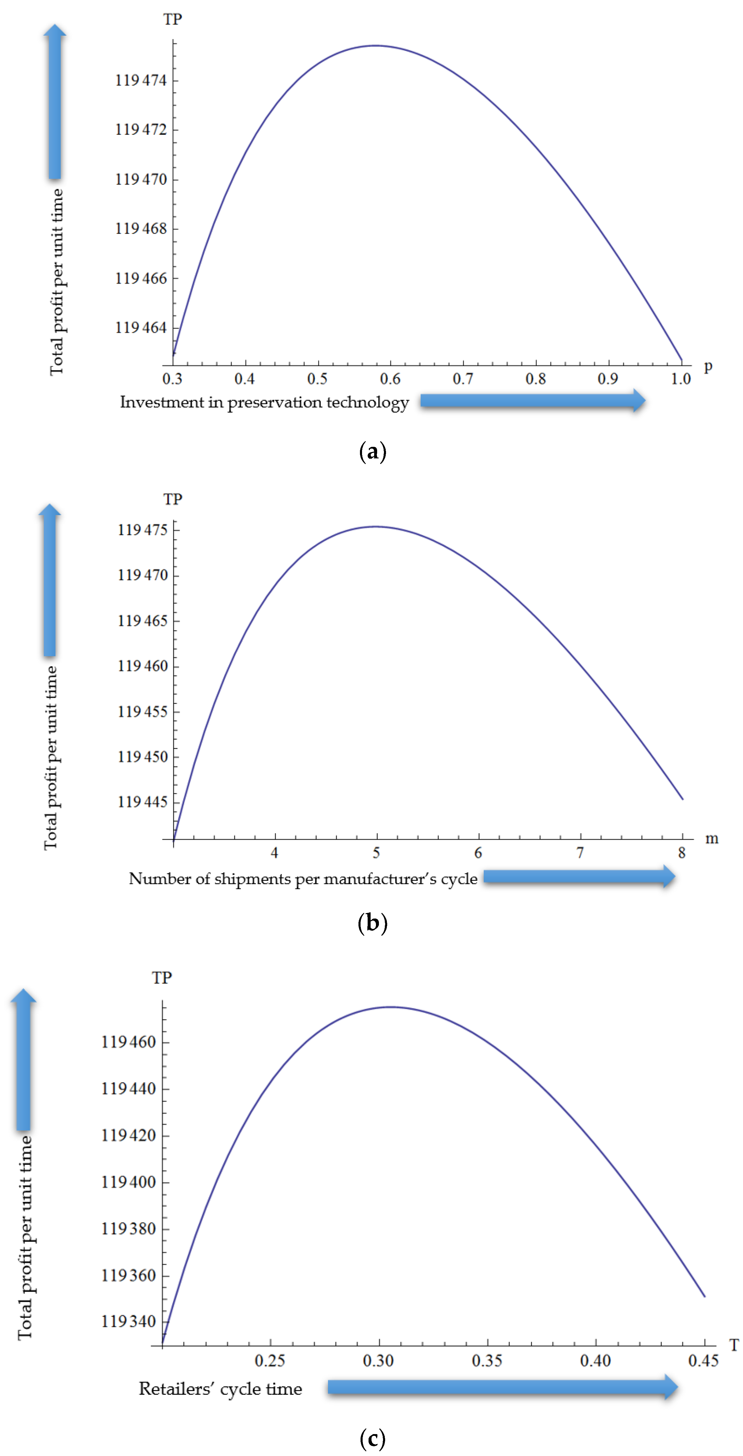
5.2.2. Results and Discussion

This section provides the optimum solution for the numerical experiments and various insights inferred from those results.

Example 1.

Single manufacturer, seven retailers, without application of preservation technology.

For this example, we considered a setup of a single manufacturer and seven retailers. The optimum values of the number of shipments/deliveries and the retailer’s cycle were computed without considering any preservation investment. By using the optimal results, the value of the total profit per unit time was calculated. The optimum results are exhibited in

Table 3. (a) Optimal solution for Example 1. (b) Optimal replenishment quantities per delivery at each retailer for Example 1. (c) Optimal solution for Example 2. (d) Optimal replenishment quantities per delivery at each retailer for Example 2.

(a)
$\begin{array}{l}T{P}^{*}\\ \$118,783/\mathrm{month}\end{array}$		$\begin{array}{l}{T}^{*}\\ 0.19 \mathrm{month}\end{array}$		$\begin{array}{l}{m}^{*}\\ 8/\mathrm{manufacturer}’\mathrm{s} \mathrm{cycle}\end{array}$
(b)
$\begin{array}{l}P{Q}_{r1}^{*}\\ 22 \mathrm{units}\end{array}$	$\begin{array}{l}P{Q}_{r2}^{*}\\ 24 \mathrm{units}\end{array}$	$\begin{array}{l}P{Q}_{r3}^{*}\\ 23 \mathrm{units}\end{array}$	$\begin{array}{l}P{Q}_{r4}^{*}\\ 20 \mathrm{units}\end{array}$	$\begin{array}{l}P{Q}_{r5}^{*}\\ 25 \mathrm{units}\end{array}$	$\begin{array}{l}P{Q}_{r6}^{*}\\ 22 \mathrm{units}\end{array}$	$\begin{array}{l}P{Q}_{r7}^{*}\\ 23 \mathrm{units}\end{array}$
(c)
$\begin{array}{l}T{P}^{*}\\ \$119,475/\mathrm{month}\end{array}$		$\begin{array}{l}{T}^{*}\\ 0.31 \mathrm{month}\end{array}$	$\begin{array}{l}{m}^{*}\\ 5/\mathrm{manufacturer}’\mathrm{s} \mathrm{cycle}\end{array}$		$\begin{array}{l}{p}^{*}\\ \$0.58/\mathrm{unit}/\mathrm{month}\end{array}$
(d)
$\begin{array}{l}P{Q}_{r1}^{*}\\ 32 \mathrm{units}\end{array}$	$\begin{array}{l}P{Q}_{r2}^{*}\\ 35 \mathrm{units}\end{array}$	$\begin{array}{l}P{Q}_{r3}^{*}\\ 34 \mathrm{units}\end{array}$	$\begin{array}{l}P{Q}_{r4}^{*}\\ 31 \mathrm{units}\end{array}$	$\begin{array}{l}P{Q}_{r5}^{*}\\ 37 \mathrm{units}\end{array}$	$\begin{array}{l}P{Q}_{r6}^{*}\\ 33 \mathrm{units}\end{array}$	$\begin{array}{l}P{Q}_{r7}^{*}\\ 35 \mathrm{units}\end{array}$

a.

From the optimal value of the retailers’ cycle time, the optimal replenishment quantity per delivery $P{Q}_{ri}$ for each retailer was calculated by using Equation (2), and the results are exhibited in Table 3b.

Table 3 shows that, in a centralized system of the proposed supply chain without the application of preservation technology, the optimal value of cycle time for a retailer is 0.19 months, which is approximately 6 days. The value of the number of deliveries/shipments to the retailers per cycle of the manufacturer is 8. From these values, the manufacturer’s cycle time is calculated as $mT=1.52 \mathrm{months}$, which is approximately 46 days. By using the values of parameters and decision variables, the maximum value of the profit is obtained, which is $118,783/month.

Example 2.

Single manufacturer, seven retailers, with application of preservation technology.

For this example, we considered a setup of a single manufacturer and seven retailers. The optimum values of the number of shipments/deliveries, retailer’s cycle time, and preservation investment were computed by considering preservation technology. By using these optimal results, the value of total profit per unit time was calculated. The optimum results are exhibited in Table 3c.

From the optimal value of cycle time, the optimal replenishment quantity per delivery $P{Q}_{ri}$ for each retailer was calculated by using Equation (2), and the results are provided in Table 3d.

Table 3d exhibits the optimal solution for Example 2. As compared to Example 1, this experiment considered the application of preservation technology. The results show that the optimal value of preservation investment was $0.58/unit/month. By applying the preservation conditions, the lifetime of the product increased from 0.5 months (15 days) to 1.4 months (42 days). As the lifetime of the product increased, retailers received larger replenishment quantities and acquired the benefit of selling the product for a longer span of time without facing serious deterioration. Therefore, the optimal value of retailers’ cycle time increased to 0.31 months, which is approximately 9 days. Likewise, due to the increased cycle time by preservation technology, the number of shipments to retailers per manufacturer’s cycle was reduced to 5 instead of 8. The manufacturer was benefited by saving the cost of transportation with the reduced number of shipments/deliveries to the retailers. The cycle time of the manufacturer is calculated as $mT=1.52 \mathrm{months}$, which is approximately 46 days. The cycle time of the manufacturer is not affected because preservation technology is applied only at the retailers’ level. The profit per unit time of the supply chain increased to $119,475/month, which was improved by approximately 0.6 percent. The optimality of these examples is depicted in Figure 4a–f.

The effect of variation in the value of total profit per unit time by varying the value of preservation investment is illustrated in Figure 4a. The profit increased with the increase in preservation investment until its optimal value, i.e., $0.58 per unit per unit time. Increasing the preservation investment beyond the optimal point means the value of profit decreases. This illustration verifies the assumption that additional preservation investment beyond a specific level does not significantly affect the rate of deterioration, and it decreases the profit by adding more to the preservation cost.

The number of shipments/deliveries to the retailers per cycle of the manufacturer indirectly affects the value of profit per unit time. This effect is exhibited in Figure 4b. For the specific numerical experiment (Example 2) the optimal number of deliveries per manufacturer’s cycle is 5. The number of deliveries more or less than 5 decreases the value of profit. As the products are deteriorating, a smaller number of deliveries to retailers per manufacturer cycle increases the retailers’ cycle time, which causes a greater number of products to deteriorate per cycle and hence decreases the profit. The number of deliveries more than the optimal value causes more transportation and handling cost, which decreases the value of profit.

The effect of variation in retailers’ cycle time on the value of profit per unit time is illustrated in Figure 4c. The inventory cycle time at the retailers’ level is an important phenomenon for deteriorating products as a greater number of items deteriorates with time. Figure 4c shows that the optimal value of retailers’ planning horizon is 0.31 months which corresponds to the maximum of the graph showing a maximum profit of $119,475 per month.

Figure 4d illustrates the joint effect of variation in the retailers’ cycle time and the number of deliveries to the retailers per manufacturer’s cycle on profit. The peak in the figure shows the maximum profit that corresponds to the optimal values of cycle time (0.31 months) and number of deliveries (5). Similarly, the dual effect of the variation in the values of preservation investment and number of shipments/deliveries to the retailers per manufacture’s cycle on the value of total supply chain profit per unit time is expounded in Figure 4e. The zenith of the graph relates to the maximum profit, i.e., $119,475 per month, which corresponds to the optimal value of preservation investment, i.e., $0.58 per unit per unit time and retailers’ cycle time, i.e., 0.31 months.

Figure 4f illustrates the combine effect of variation in the values of preservation investment and retailers’ planning horizon on profit. The peak of the graph corresponds to the maximum value of the profit, i.e., $119,475 per month, which relates to the optimal values of preservation investment, i.e., $0.58 per unit per unit time and that of retailers’ cycle time, i.e., 0.31 months.

Comparative Analysis of the Results from Examples 1 and 2

As observed from both the numerical experiments, the optimal values of the results change when preservation technology is applied. To provide more insights into these variations, a comparative analysis was performed for some critical results from both the examples. The results of the comparative analysis are exhibited below in

Table 4. (a) Comparative analysis of important results with and without preservation technology. (b) Optimal replenishment quantities per delivery at each retailer.

(a)
Parameters		Without Preservation		With Preservation		Percent Variation
Lifetime (month/s)		0.5		1.4		180
Cycle time (month/s)		0.19		0.31		63
Number of shipments		8		5		−37.5
Profit/month ($/month)		118,783		119,475		0.58
(b)
$\begin{array}{l}P{Q}_{r1}^{*}\\ 195 \mathrm{units}\end{array}$	$\begin{array}{l}P{Q}_{r2}^{*}\\ 214 \mathrm{units}\end{array}$	$\begin{array}{l}P{Q}_{r3}^{*}\\ 204 \mathrm{units}\end{array}$	$\begin{array}{l}P{Q}_{r4}^{*}\\ 185 \mathrm{units}\end{array}$	$\begin{array}{l}P{Q}_{r5}^{*}\\ 224 \mathrm{units}\end{array}$	$\begin{array}{l}P{Q}_{r6}^{*}\\ 199 \mathrm{units}\end{array}$	$\begin{array}{l}P{Q}_{r7}^{*}\\ 210 \mathrm{units}\end{array}$

a.

The comparative analysis of the optimal results with and without preservation shows that the application of preservation technology increases the lifetime of the product, retailers’ cycle time, and total profit per unit time of the proposed supply chain, while the number of shipments/deliveries to the retailers per manufacturer’s cycle are reduced. These variations are illustrated in Figure 5a. An improved lifetime ensures that the food products are delivered to the consumers as fresh. Similarly, an increased replenishment cycle at the retailer provides them more time to sell the products without facing serious deterioration which makes them earn more profit. The results show that without applying preservation technology, the profit and cycle time are decreased, while the number of deliveries/shipments are increased. The decrease in optimal value of cycle time is a significant insight for supply chains of deteriorating products. As the products are deteriorating, therefore, without preservation, the rate of deterioration increases, and products deteriorate quickly. Thus, at the retailers’ level, shorter spans of inventory replenishment are more optimal as compared to longer spans. Due to the same reasons, the number of deliveries/shipments from the manufacturer to the retailers are increased in order to avoid losses due to deterioration. In the case of a fewer number of shipments, products stay as inventory for a longer time and a greater number of products deteriorate at the retailer. Therefore, it is more advantageous to reduce the delivery size and increase the number of deliveries, so that a greater number of items could be sold before their expiration.

The profit of the system increases with the application of preservation technology. Moreover, the transportation cost can be saved with the reduced number of shipments when preservation technology is applied, which will add a greater amount to the profit. From an economic point of view, this analysis suggests that the retailers should adopt preservation technology for the supply chains of deteriorating products that will not only increase the profit but also allow the retailers to sell their products for a longer time without facing significant deterioration.

Example 3.

A special case of Example 2 by considering single shipment to retailers per manufacturer’s cycle, keeping the cycle time of retailers as per manufacturer’s cycle time.

In this case, Example 2 is modified to consider the single setup single delivery (SSSD) policy. Therefore, the value of $m$ is taken as 1 and the value of the retailers’ cycle time is considered equal to that of the manufacturer, i.e., the value of $T$ is taken as 1.52 months. The solution is obtained for the optimal preservation investment and the maximum profit per month is computed. The optimal investment in preservation $p^{*}$ is $0.66 per unit per month, and the maximum value of profit $T{P}^{*}$ is $117,020 per month. The lot size for each retailer is computed and exhibited in Table 4b.

There is a noticeable difference in the optimal values of preservation investment, lot sizes, and profit per unit time for this case when compared to the results from Example 2. The value of the profit per unit time decreased by 2.04% and that of the optimal preservation investment increased by 12.65%. This is a remarkable variation, which is caused by the results of increased deterioration. Adopting the SSSD policy, the inventory replenishment schedule is delayed, and larger-sized lots of the product remain with retailers for longer periods of time. Due to the decaying nature, a greater number of items deteriorate. Such situations call for more preservation investment as is evident from the results. Likewise, due to more deterioration and increased preservation investment, the profit per unit time decreases. These variations are illustrated in Figure 5b. The comparative analysis of the results from both the examples proves that the SSMD policy is a better choice for deteriorating products in a multiple retailer centralized supply chain system, where it increases the profit as well as continuing to deliver the food products fresher to the consumers by increasing the lifetime and reducing deterioration.

5.2.3. Sensitivity Analysis

To estimate the effects of variation in the value of the key cost parameters on the profit value and decision variables, a sensitivity analysis was performed on Example 2. The results of the sensitivity analysis are exhibited in

Table 5. Sensitivity analysis of key cost parameters for Example 2.

Percentage Variation in Parameters		Percentage Variation in Optimal Values of Decision Variables and Profit
		$\mathit{m}$	$\mathit{p}$	$\mathit{T}$	$\mathit{T}\mathit{P}$
$C_{mt}$	−50	−20	−31.21	14.52	3.23
	−25	0	−15.69	5.48	1.61
	25	0	14.83	−7.42	−1.60
	50	20	29.83	−11.94	−3.20
$C_p$	−50	0	−15.69	5.48	1.61
	−25	0	−7.93	1.61	0.80
	25	0	7.24	−4.52	−0.80
	50	0	14.83	−7.42	−1.60
$A_{r1}$	−50	0	−0.52	−4.68	0.04
	−25	0	−0.34	−3.55	0.02
	25	0	−0.34	10.32	−0.02
	50	0	−0.17	1.94	−0.04
$h_{r1}$	−50	0	−0.34	−1.61	0.00
	−25	0	−0.34	−1.29	0.00
	25	0	−0.34	−1.61	0.00
	50	0	−0.34	−1.94	0.00
$h_m$	−50	40	−0.69	−1.29	0.06
	−25	20	−0.52	−1.61	0.03
	25	−20	−0.17	−1.61	−0.03
	50	−40	−0.17	−1.61	−0.05
$C_{set}$	−50	−20	−0.69	−1.61	0.06
	−25	−20	−0.52	−1.61	0.03
	25	20	−0.17	−1.61	−0.03
	50	20	−0.17	−1.61	−0.05

.

The results of the sensitivity analysis are discussed below.

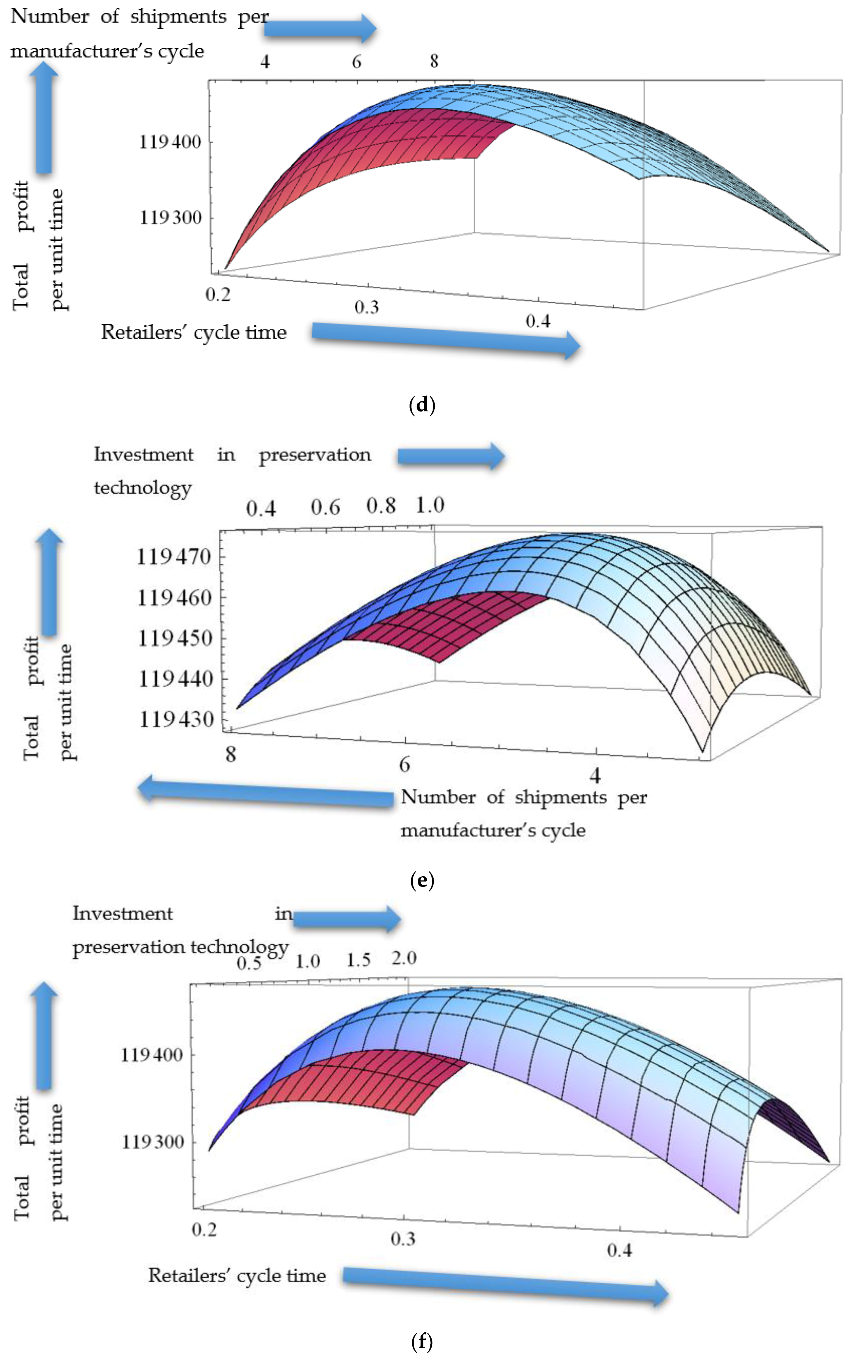
• The magnitude of variation in the value of profit is different from the variation in different cost parameters. The effect of variation in the value of each cost parameter on the value of profit is illustrated in Figure 5c.
• The cost of production and the cost of materials affect the profit the most, while the variation in the value of inventory holding cost of retailer 1 has no effect on the value of the profit. Other cost parameters including manufacturer’s setup cost and inventory holding cost, and retailer’s ordering cost have an insignificant effect on the value of profit.
• Variations in production and material cost have a significant and inverse effect on the value of the retailers’ cycle time. The cycle time varies directly with variations in the retailer’s ordering cost. Retailers’ and manufacturers’ inventory holding costs and setup costs of manufacture have no significant effect on the value of the cycle time.
• The investment in the preservation is affected directly by the variation in the cost parameters. This effect is significant for cost of material and production cost, while other cost parameters do not have a considerable effect on the value of preservation investment.
• Variations in production cost, retailer’s ordering, and inventory holding cost have no effect on the value of the number of deliveries/shipments to the retailers per cycle of the manufacturer. Variations in the cost of material affect directly, while that in the manufacturer’s inventory holding cost and setup cost affect the number of shipments/deliveries inversely.

6. Managerial Insights

This model is applicable for the industries comprising single production and multiple retailers’ setup, the produce of which is deteriorating products. Managers of such setups strive to reduce the costs and keep the freshness of the products at various stages of the supply chain. This model can help those managers to achieve their objectives by providing an optimum level of preservation and multiple shipment policies, thus benefiting all the players of the supply chains, and satisfying their customers with the best quality.

6.1. Insight 1—Transportation/Delivery Reduction

The rate of deterioration improves when preservation is used at retailers. Investing an optimum amount in preservation technology not only improves the profit but also increases the lot size per shipment/delivery. In such situations, managers should consider those delivery trucks, which can deliver larger shipments to the retailers. Moreover, as the cycle time of all the retailers is fixed to be equal, the transportation activities should be accomplished in a way such that the same delivery trucks deliver the consignments to all the retailers in one loop, thus minimizing the route distance, such that the cost of transportation be minimum. The reduced number of deliveries also helps to avoid environmental pollution which affects the life of human beings positively. Moreover, the location of the retailing points is considerable while transporting the fresh food products, as suggested by Liu et al. [62].

6.2. Insight 2—Demand Improvement

This research assumed different demands at each retailer due to the behavior of customers within a specific region and location of the retailer. Each retailer can increase the demand at their stores by doing local advertisements and consumer analysis. Therefore, retail managers should carry out such advertisement practices within their area, so that the sales be increased, and profit is improved. Besides, the selling price is also a critical factor that affects the demand for a product. Managers can use such innovative tools in collaboration with the consumers to increase their sales. This not only increases sales but also contributes to environmental sustainability. Such innovative and sustainable solutions can be achieved by engaging buyers in green product development.

6.3. Insight 3—Profit Maximization

The prime objective of the companies is to earn more profit by utilizing their resources efficiently. Therefore, the managers of supply chains attempt to reduce several costs to maximize the total profit. It is inferred from the numerical results that the production and material costs affect the profit significantly. Thus, reducing these costs can improve the profit significantly. On the other side, a decrease in any of these costs affects the other costs. For example, a decrease in material cost reduces the quality of raw material, which increases the production cost by producing more waste items. Similarly, a reduced production cost produces more defective items, which ultimately calls for consuming a higher amount of raw material to complete the production order. Therefore, managers should improve these costs by improving the supplier selection process as well as improving the production system [63].

6.4. Insight 4—Preservation during Transportation

As products under consideration are deteriorating in nature, therefore, it may be necessary to provide preservation technology during transportation in some cases, e.g., for products such as ice cream, etc. Thus, the managers should consider such costs within the cost of transportation. As is demonstrated by the results, shorter cycles of inventory replenishments are more optimal for such deteriorating products. This will help to keep the food products fresh for the consumers.

6.5. Insight 5—Environmental Protection

An important insight of this study is environmental sustainability. The products that deteriorated without effective preservation policies have adverse effects on the environment. As a large an amount of waste as 33% of the total food produced in the world is alarming, significantly disturbing the environmental balance and ultimately affecting the life of human beings. The ultimate target of zero pollution can only be achieved by eliminating food waste by using effective preservation policies and improving eating habits.

7. Conclusions

This study proposed a supply chain model for deteriorating products, where a single manufacturer delivers finished products to multiple retailers in multiple shipments by considering SSMD policy and unequal lot size. The rate of deterioration is minimized at retailers with the help of preservation technology. The preservation investment decreased the rate of deterioration, but the magnitude of the decrease in deterioration decreased with additional preservation investment. The proposed study addressed the effect of preservation technology on a product’s lifetime, rate of deterioration, retailers’ cycle time, number of deliveries to the retailers per manufacturer’s cycle, and profit of the system. It was proved that the optimum level of preservation technology significantly improved the profit and lifetime of the product. Besides, due to the reduced rate of deterioration by preservation, the optimum value of the lot size and that of the retailers’ replenishment cycle increased, while the number of replenishment/deliveries decreased, which not only reduced the cost of transportation, but also provided retailers with more time to sell their products without facing serious deterioration. This research examined the effect of the number of deliveries/replenishments on preservation investment and the profit of the system. The results of the experiments proved that the optimum number of replenishments/deliveries required less preservation investment, while generating more profit, as compared to a single delivery system (SSSD policy). It can be comprehensively concluded that the SSMD policy takes advantage over the SSSD policy and preservation investment is profitable for fresh food products within such a setup.

Limitations and Future Research Directions

This study has been conducted comprehensively to study the effects of preservation, shipment cycle, and number of shipments within the SSMD setup considering unequal lot size. However, there are some limitations, which can be addressed as future research avenues.

• This research considered variable ordering cost, inventory holding cost, and selling price due to several demographical, geographical, and setup structure reasons, which can be modeled to extend this research.
• As the demand at each retailer is assumed to be different due to several reasons, those reasons can be considered and modeled to improve the customer demand, e.g., by considering local advertisement-dependent demand for each retailer, as considered by Palanivel and Uthayakumar [64].
• This research assumed a constant size of each replenishment for a single retailer, which can be considered as different for each replenishment, as proposed by Goyal [16].
• The proposed model considered that uniform preservation investment though the lot size is different at each retailer. This model can be extended by relating the amount of preservation investment to the lot size.

References

1. Gustavsson, J.; Cederberg, C.; Sonesson, U.; Van Otterdijk, R.; Meybeck, A. Global Food Losses and Food Waste; FAO: Rome, Italy, 2011. [Google Scholar]
2. Hill, R.; Omar, M. Another look at the single-vendor single-buyer integrated production-inventory problem. Int. J. Prod. Res. 2006, 44, 791–800. [Google Scholar] [CrossRef]
3. Yang, P.; Chung, S.; Wee, H.; Zahara, E.; Peng, C. Collaboration for a closed-loop deteriorating inventory supply chain with multi-retailer and price-sensitive demand. Int. J. Prod. Econ. 2013, 143, 557–566. [Google Scholar] [CrossRef]
4. Tantiwattanakul, P.; Dumrongsiri, A. Supply chain coordination using wholesale prices with multiple products, multiple periods, and multiple retailers: Bi-level optimization approach. Comput. Ind. Eng. 2019, 131, 391–407. [Google Scholar] [CrossRef]
5. Chan, C.K.; Fang, F.; Langevin, A. Single-vendor multi-buyer supply chain coordination with stochastic demand. Int. J. Prod. Econ. 2018, 206, 110–133. [Google Scholar] [CrossRef]
6. Azadi, Z.; Eksioglu, S.D.; Eksioglu, B.; Palak, G. Stochastic optimization models for joint pricing and inventory replenishment of perishable products. Comput. Ind. Eng. 2019, 127, 625–642. [Google Scholar] [CrossRef]
7. Sufiyan, M.; Haleem, A.; Khan, S.; Khan, M.I. Evaluating food supply chain performance using hybrid fuzzy MCDM technique. Sustain. Prod. Consum. 2019, 20, 40–57. [Google Scholar] [CrossRef]
8. Sarkar, S.; Tiwari, S.; Giri, B. Impact of uncertain demand and lead-time reduction on two-echelon supply chain. Ann. Oper. Res. 2021, 1–29. [Google Scholar] [CrossRef]
9. Ananno, A.A.; Masud, M.H.; Chowdhury, S.A.; Dabnichki, P.; Ahmed, N.; Arefin, A.M.E. Sustainable food waste management model for Bangladesh. Sustain. Prod. Consum. 2021, 27, 35–51. [Google Scholar] [CrossRef]
10. Jeswani, H.K.; Figueroa-Torres, G.; Azapagic, A. The extent of food waste generation in the UK and its environmental impacts. Sustain. Prod. Consum. 2021, 26, 532–547. [Google Scholar] [CrossRef]
11. Ben-Daya, M.; As’ad, R.; Seliaman, M. An integrated production inventory model with raw material replenishment considerations in a three layer supply chain. Int. J. Prod. Econ. 2013, 143, 53–61. [Google Scholar] [CrossRef]
12. Cárdenas-Barrón, L.E. Optimizing inventory decisions in a multi-stage multi-customer supply chain: A note. Transp. Res. Part E Logist. Transp. Rev. 2007, 43, 647–654. [Google Scholar] [CrossRef]
13. Goyal, S.K. “A joint economic-lot-size model for purchaser and vendor”: A comment. Decis. Sci. 1988, 19, 236–241. [Google Scholar] [CrossRef]
14. Banerjee, A. A joint economic-lot-size model for purchaser and vendor. Decis. Sci. 1986, 17, 292–311. [Google Scholar] [CrossRef]
15. Lu, L. A one-vendor multi-buyer integrated inventory model. Eur. J. Oper. Res. 1995, 81, 312–323. [Google Scholar] [CrossRef]
16. Goyal, S.K. A one-vendor multi-buyer integrated inventory model: A comment. Eur. J. Oper. Res. 1995, 82, 209–210. [Google Scholar] [CrossRef]
17. Thomas, D.J.; Griffin, P.M. Coordinated supply chain management. Eur. J. Oper. Res. 1996, 94, 1–15. [Google Scholar] [CrossRef]
18. Hill, R.M. The single-vendor single-buyer integrated production-inventory model with a generalised policy. Eur. J. Oper. Res. 1997, 97, 493–499. [Google Scholar] [CrossRef]
19. Hill, R.M. The optimal production and shipment policy for the single-vendor singlebuyer integrated production-inventory problem. Int. J. Prod. Res. 1999, 37, 2463–2475. [Google Scholar] [CrossRef]
20. Goyal, S.K.; Nebebe, F. Determination of economic production–shipment policy for a single-vendor–single-buyer system. Eur. J. Oper. Res. 2000, 121, 175–178. [Google Scholar] [CrossRef]
21. Yang, P.-C.; Wee, H.-M. A single-vendor and multiple-buyers production–inventory policy for a deteriorating item. Eur. J. Oper. Res. 2002, 143, 570–581. [Google Scholar] [CrossRef]
22. Khouja, M. Optimizing inventory decisions in a multi-stage multi-customer supply chain. Transp. Res. Part E Logist. Transp. Rev. 2003, 39, 193–208. [Google Scholar] [CrossRef]
23. Wang, S.; Sarker, B.R. An assembly-type supply chain system controlled by kanbans under a just-in-time delivery policy. Eur. J. Oper. Res. 2005, 162, 153–172. [Google Scholar] [CrossRef]
24. Siajadi, H.; Ibrahim, R.N.; Lochert, P.B. A single-vendor multiple-buyer inventory model with a multiple-shipment policy. Int. J. Adv. Manuf. Technol. 2006, 27, 1030–1037. [Google Scholar] [CrossRef]
25. Chan, C.K.; Kingsman, B.G. Coordination in a single-vendor multi-buyer supply chain by synchronizing delivery and production cycles. Transp. Res. Part E Logist. Transp. Rev. 2007, 43, 90–111. [Google Scholar] [CrossRef]
26. Ben-Daya, M.; Al-Nassar, A. An integrated inventory production system in a three-layer supply chain. Prod. Plan. Control 2008, 19, 97–104. [Google Scholar] [CrossRef]
27. Darwish, M.A.; Odah, O. Vendor managed inventory model for single-vendor multi-retailer supply chains. Eur. J. Oper. Res. 2010, 204, 473–484. [Google Scholar] [CrossRef]
28. Roy, M.D.; Sana, S.S.; Chaudhuri, K. An optimal shipment strategy for imperfect items in a stock-out situation. Math. Comput. Model. 2011, 54, 2528–2543. [Google Scholar]
29. Sajadieh, M.S.; Fallahnezhad, M.S.; Khosravi, M. A joint optimal policy for a multiple-suppliers multiple-manufacturers multiple-retailers system. Int. J. Prod. Econ. 2013, 146, 738–744. [Google Scholar] [CrossRef]
30. Sana, S.S.; Chedid, J.A.; Navarro, K.S. A three layer supply chain model with multiple suppliers, manufacturers and retailers for multiple items. Appl. Math. Comput. 2014, 229, 139–150. [Google Scholar] [CrossRef]
31. Yang, G.-Q.; Liu, Y.-K.; Yang, K. Multi-objective biogeography-based optimization for supply chain network design under uncertainty. Comput. Ind. Eng. 2015, 85, 145–156. [Google Scholar] [CrossRef]
32. Jia, T.; Liu, Y.; Wang, N.; Lin, F. Optimal production-delivery policy for a vendor-buyers integrated system considering postponed simultaneous delivery. Comput. Ind. Eng. 2016, 99, 1–15. [Google Scholar] [CrossRef]
33. Song, Y.; Fan, T.; Tang, Y.; Xu, C. Omni-channel strategies for fresh produce with extra losses in-store. Transp. Res. Part E Logist. Transp. Rev. 2021, 148, 102243. [Google Scholar] [CrossRef]
34. Ghare, P.; Schrader, G. A model for exponentially decaying inventory. J. Ind. Eng. 1963, 14, 238–243. [Google Scholar]
35. Sachan, R. On (T, S i) policy inventory model for deteriorating items with time proportional demand. J. Oper. Res. Soc. 1984, 35, 1013–1019. [Google Scholar]
36. Chang, H.-J.; Dye, C.-Y. An EOQ model for deteriorating items with time varying demand and partial backlogging. J. Oper. Res. Soc. 1999, 50, 1176–1182. [Google Scholar] [CrossRef]
37. Skouri, K.; Konstantaras, I.; Papachristos, S.; Ganas, I. Inventory models with ramp type demand rate, partial backlogging and Weibull deterioration rate. Eur. J. Oper. Res. 2009, 192, 79–92. [Google Scholar] [CrossRef]
38. Shah, N.H.; Soni, H.N.; Patel, K.A. Optimizing inventory and marketing policy for non-instantaneous deteriorating items with generalized type deterioration and holding cost rates. Omega 2013, 41, 421–430. [Google Scholar] [CrossRef]
39. Wu, J.; Ouyang, L.-Y.; Cárdenas-Barrón, L.E.; Goyal, S.K. Optimal credit period and lot size for deteriorating items with expiration dates under two-level trade credit financing. Eur. J. Oper. Res. 2014, 237, 898–908. [Google Scholar] [CrossRef]
40. Qin, Y.; Wang, J.; Wei, C. Joint pricing and inventory control for fresh produce and foods with quality and physical quantity deteriorating simultaneously. Int. J. Prod. Econ. 2014, 152, 42–48. [Google Scholar] [CrossRef]
41. Iqbal, M.W.; Sarkar, B. Recycling of lifetime dependent deteriorated products through different supply chains. RAIRO-Oper. Res. 2019, 53, 129–156. [Google Scholar] [CrossRef]
42. Iqbal, M.W.; Sarkar, B. Application of preservation technology for lifetime dependent products in an integrated production system. J. Ind. Manag. Optim. 2020, 16, 141. [Google Scholar] [CrossRef] [Green Version]
43. Chen, S.-C.; Teng, J.-T. Retailer’s optimal ordering policy for deteriorating items with maximum lifetime under supplier’s trade credit financing. Appl. Math. Model. 2014, 38, 4049–4061. [Google Scholar] [CrossRef]
44. Wang, W.-C.; Teng, J.-T.; Lou, K.-R. Seller’s optimal credit period and cycle time in a supply chain for deteriorating items with maximum lifetime. Eur. J. Oper. Res. 2014, 232, 315–321. [Google Scholar] [CrossRef]
45. Shah, N.H.; Chaudhari, U.; Jani, M.Y. Optimal policies for time-varying deteriorating item with preservation technology under selling price and trade credit dependent quadratic demand in a supply chain. Int. J. Appl. Comput. Math. 2016, 3, 363–379. [Google Scholar] [CrossRef]
46. Feng, L.; Chan, Y.-L.; Cárdenas-Barrón, L.E. Pricing and lot-sizing polices for perishable goods when the demand depends on selling price, displayed stocks, and expiration date. Int. J. Prod. Econ. 2017, 185, 11–20. [Google Scholar] [CrossRef]
47. Chen, J.; Dong, M.; Xu, L. A perishable product shipment consolidation model considering freshness-keeping effort. Transp. Res. Part E Logist. Transp. Rev. 2018, 115, 56–86. [Google Scholar] [CrossRef]
48. Daryanto, Y.; Wee, H.M.; Astanti, R.D. Three-echelon supply chain model considering carbon emission and item deterioration. Transp. Res. Part. E Logist. Transp. Rev. 2019, 122, 368–383. [Google Scholar] [CrossRef]
49. Iqbal, M.W.; Kang, Y.; Jeon, H.W. Zero waste strategy for green supply chain management with minimization of energy consumption. J. Clean. Prod. 2020, 245, 118827. [Google Scholar] [CrossRef]
50. Hsu, P.; Wee, H.; Teng, H. Preservation technology investment for deteriorating inventory. Int. J. Prod. Econ. 2010, 124, 388–394. [Google Scholar] [CrossRef]
51. Dye, C.-Y. The effect of preservation technology investment on a non-instantaneous deteriorating inventory model. Omega 2013, 41, 872–880. [Google Scholar] [CrossRef]
52. He, Y.; Huang, H. Optimizing inventory and pricing policy for seasonal deteriorating products with preservation technology investment. J. Ind. Eng. 2013, 2013, 793568. [Google Scholar] [CrossRef]
53. Yang, C.-T.; Dye, C.-Y.; Ding, J.-F. Optimal dynamic trade credit and preservation technology allocation for a deteriorating inventory model. Comput. Ind. Eng. 2015, 87, 356–369. [Google Scholar] [CrossRef]
54. Tsao, Y.-C. Designing a supply chain network for deteriorating inventory under preservation effort and trade credits. Int. J. Prod. Res. 2016, 54, 3837–3851. [Google Scholar] [CrossRef]
55. Dye, C.-Y.; Yang, C.-T. Optimal dynamic pricing and preservation technology investment for deteriorating products with reference price effects. Omega 2016, 62, 52–67. [Google Scholar] [CrossRef]
56. Giri, B.; Pal, H.; Maiti, T. A vendor-buyer supply chain model for time-dependent deteriorating item with preservation technology investment. Int. J. Math. Oper. Res. 2017, 10, 431–449. [Google Scholar] [CrossRef]
57. Mishra, U.; Wu, J.-Z.; Tsao, Y.-C.; Tseng, M.-L. Sustainable inventory system with controllable non-instantaneous deterioration and environmental emission rates. J. Clean. Prod. 2020, 244, 118807. [Google Scholar] [CrossRef]
58. Khakzad, A.; Gholamian, M.R. The effect of inspection on deterioration rate: An inventory model for deteriorating items with advanced payment. J. Clean. Prod. 2020, 254, 120117. [Google Scholar] [CrossRef]
59. Woo, Y.Y.; Hsu, S.-L.; Wu, S. An integrated inventory model for a single vendor and multiple buyers with ordering cost reduction. Int. J. Prod. Econ. 2001, 73, 203–215. [Google Scholar] [CrossRef]
60. Ertogral, K.; Darwish, M.; Ben-Daya, M. Production and shipment lot sizing in a vendor–buyer supply chain with transportation cost. Eur. J. Oper. Res. 2007, 176, 1592–1606. [Google Scholar] [CrossRef]
61. Iqbal, M.W.; Kang, Y. Waste-to-energy supply chain management with energy feasibility condition. J. Clean. Prod. 2021, 291, 125231. [Google Scholar] [CrossRef]
62. Liu, A.; Zhu, Q.; Xu, L.; Lu, Q.; Fan, Y. Sustainable supply chain management for perishable products in emerging markets: An integrated location-inventory-routing model. Transp. Res. Part E Logist. Transp. Rev. 2021, 150, 102319. [Google Scholar] [CrossRef]
63. Bragg, S.M. Production Cost Reduction. In Cost Reduction Analysis: Tools and Strategies; John Wiley & Sons: Hoboken, NJ, USA, 2010; pp. 91–105. [Google Scholar]
64. Palanivel, M.; Uthayakumar, R. Finite horizon EOQ model for non-instantaneous deteriorating items with price and advertisement dependent demand and partial backlogging under inflation. Int. J. Syst. Sci. 2015, 46, 1762–1773. [Google Scholar] [CrossRef]
Figure 1. Problem structure (single manufacturer and multiple retailers).
Sustainability 14 06782 g001
Figure 2. (a) Reduced effect of additional investment in preservation technology on lifetime. (b) Reduced effect of additional investment in preservation technology on deterioration.
Sustainability 14 06782 g002
Figure 3. (a) Behavior of inventory level per cycle at i th retailer. (b) Behavior of inventory level per manufacturer’s cycle.
Sustainability 14 06782 g003
Figure 4. (a) Total profit per unit time versus investment in preservation technology. (b) Total profit per unit time versus number of replenishments per manufacturer’s cycle. (c) Total profit per unit time versus retailers’ cycle time. (d) Total profit per unit time versus retailers’ cycle time and number of shipments/deliveries to retailers per manufacturer’s cycle. (e) Total profit per unit time versus investment in preservation technology and number of shipments/deliveries to retailers per manufacturer’s cycle. (f) Total profit per unit time versus investment in preservation technology and retailers’ cycle time.
Sustainability 14 06782 g004aSustainability 14 06782 g004b
Figure 5. (a) Improvement in product’s lifetime, retailers’ cycle time, number of shipments, lot size, and profit with investment in preservation technology. (b) Losses when SSSD policy is adopted instead of SSMD policy. (c) Variation in profit per unit time by varying retailer 1′s ordering cost, inventory holding cost, manufacturer’s setup cost, production cost, inventory holding cost, and material cost.
Sustainability 14 06782 g005