Article

Association between Atrial Fibrillation Incidence and Temperatures, Wind Scale and Air Quality: An Exploratory Study for Shanghai and Kunming

1
Business School, University of Shanghai for Science and Technology, 516 Jungong Road, Shanghai 200093, China
2
Shanghai Key Laboratory of Interventional Medical Devices and Equipment, 1601 Zhangdong Road, Shanghai 201203, China
*
Author to whom correspondence should be addressed.
Co-first author, these authors contributed equally to this work.
Sustainability 2021, 13(9), 5247; https://doi.org/10.3390/su13095247
Submission received: 3 April 2021 / Revised: 2 May 2021 / Accepted: 5 May 2021 / Published: 7 May 2021
(This article belongs to the Collection Air Pollution Control and Sustainable Development)

Abstract

:
As a common cardiovascular disease, atrial fibrillation has the characteristics of high morbidity, high disability, and high fatality rates, seriously endangering human health and sustainability. Some research has confirmed that environmental factors are related to the risk of illness and death from cardiovascular diseases (including atrial fibrillation), while there is still little comparison on the situation of the two cities in China. This research uses medical data in Shanghai and Kunming establishing, through two-step research, logistic models to compare the impacts on atrial fibrillation incidence to figure out the association between environmental factors (including air pollution, weather, temperature, and wind scales) and atrial fibrillation. Finally, this research shows that environmental impacts on atrial fibrillation prevalence have generality, regionality, and lagging characteristics. The result is significant for atrial fibrillation patients and provides a reliable medical theory basis for nursing measures. Besides, this research provides a prospective method of offering early warning for potential atrial fibrillation patients, helping to maintain human beings’ sustainable development.

1. Introduction

Atrial fibrillation (AF) is a disease that seriously endangers human health, recognized as a common complication of cardiovascular diseases. AF refers to the loss of routine and regular diastolic and contraction activities of the heart muscle, replaced by fast and uncoordinated weak peristalsis, causing the atrium to lose normal and effective contraction. Hence, blood tends to stagnate in the atrium and form a thrombus. The prevalence of AF in adults is about 3.0%, increasing with age and cardiovascular complications. In 2010, there were 33.5 million patients with AF worldwide. In the European Union and the United States, about one quarter of middle-aged people may suffer from AF [1]. In contrast, studies declare that AF’s prevalence in China has increased by 20 times in the past ten years [2]. The total AF prevalence rate of people over 35 years old is 0.7%, and that of people over 80 is 7.5%, with the overall patient population reaching 4.87 million; however, 34.0% of them do not realize their AF history [3,4].
What is more, AF has seriously affected the sustainable development of human life. All-cause mortality caused by AF has increased by 1.5 times in men and 2 times in women [1]. Thromboembolic complications are the leading cause of death and disability in AF, and stroke is the most common manifestation, where strokes caused by AF account for 20.0% of all strokes [5,6,7]. Compared with non-AF-related strokes, AF-related strokes have severe symptoms, high disability, high mortality, and high recurrence. Its fatality rate is twice that of non-AF-related stroke [8].
As an essential part of the natural environment, climate profoundly impacts the global natural ecosystem and socio-economic system and even restricts all humankind’s sustainable development. At present, many studies have confirmed that the lag-pattern impact of air pollutants may lead to the number of outpatients increasing, especially those who come to the hospital due to cardiovascular diseases, and an increase in the death rate of patients [9,10]. Besides, many governments have highlighted the importance of protecting the environment through sustainable development, wherein the air pollution index is vital [11,12]. With the increasing consciousness of air pollution’s impact on human health [13,14], many scholars have focused on researching the association between air pollutant concentration and cardiovascular disease (CVD) prevalence. Nevertheless, as a sub-category of CVD, the association between environmental factors and AF are less concentrated. Therefore, this paper concentrates on the impact of environmental factors, researching the association between environmental factors and AF incidence to protect human health and provide early warnings.

2. Literature Review and Research Gap

Deeply researching and comprehending the impact of air pollution on the prevalence of AF is of significance. As AF is a sub-category of CVD, many scholars concentrate on researching the relationship between air pollution and CVD. Epidemiological studies have confirmed that air pollution impacts the cardiovascular system, and changes in air pollution concentrations are significantly related to the mortality and morbidity of CVD [15,16,17,18]. The previous research points out that every 10 µg/m3 increase in the concentration of PM10 in the air would increase the death rate from cardiovascular diseases by 2.4% [19], where PM10 denotes particulate matter (PM) with aerodynamic diameters ≤ 10 μm, with the unit of concentration being µg/m3. Similarly, a study evaluated the effects of long-term exposure to air pollution on Seoul residents’ cardiovascular system, which carried out a 7-year follow-up of 136,094 participants in Seoul, asserting that the risk of cardiovascular events increased linearly with the increase in the average concentration of PM2.5 [20], where FPM2.5 denotes PM with aerodynamic diameters ≤ 2.5 μm, recognized as a significant part of the total suspended particulate (TSP) as PM10 above, with the unit of concentration being µg/m3. Besides, a prospective cohort study of 189,793 men over the age of 40 in 45 regions of China figured out that for every 10 μg/m3 increase in PM2.5, cardiovascular disease mortality increased by 9% [21]. Similarly, in 2010, the American Heart Association (AHA) published the scientific statement Air Pollution and Cardiovascular Diseases, stating that fine particulate matter exposure can lead to an increase in the incidence and mortality of CVD; therefore, fine particulate matter exposure is considered to be a form of controllable risk factor for the disease [21]. To sum up, it is of significance to develop the impact of air pollution on the prevalence of AF.
As a common complication of CVD, the prevalence of AF is considerably affected by air pollution, proven by many scholars. Studies have shown that in the general population of Asia, long-term exposure to PM2.5 is associated with an increased incidence of new-onset AF, and the situation for obese male subjects over 60 years of age with a history of hypertension or myocardial infarction is more serious [22]. It could be explained as ambient air pollution being positively correlated with elevated blood pressure and hypertension [23]. Furthermore, the Chinese Cardiovascular Health and Disease Report of 2019 points out, a series of studies based on daily data of air pollution and causes of death from 2013 to 2015 in 272 cities in China found that PM2.5, O3, SO2, and NO2 increased by 10 μg/m³, and for every 1 mg/m3 increase in CO, the risk of cardiovascular death increased by 0.3%, 0.3%, 0.7%, 0.9%, and 1.1%, respectively [24,25,26,27,28].
Different research figured out a similar result: air pollution’s impact has a lag-effect pattern. For example, Kim et al. point out that the number of lag days for PM2.5’s effect on CVD depends on its chemical composition, and different lag times may vary with the patient’s health status and disease [29]. Moreover, the correlation between PM2.5 and CVD mortality mainly occurred in the first 6 days, and the relationship between them lag from 0.5 to 3 days, and mortality was the largest [30].
Adding weather and wind scales into consideration, previous researchers have more specific conclusions. Y Ma et al. focused on the relationship between different air pollutants and the incidence of CVD on sandy and dusty days, and announced that PM10 and SO2 lag 1 day, and NO2 lags 2 days [31]. Research by Su Chang et al. asserts that the association between air pollutants and CVD incidence is more substantial in spring and winter, and the wind indirectly affects the incidence of CVD; meanwhile, the study also observed that the reduction in air pollution levels led to a reduction in the incidence of CVD [32]. Similarly, Ghanizadeh G et al. collected 1021 articles and pointed out that climate change parameters such as temperature, humidity, and air pollution significantly affect cardiorespiratory health [33]. What is more, it has been proven that meteorological fluctuations are most related to heart failure in the first 3 days of hospitalization, and that temperature and heart failure have a two-way relationship [34].
To sum up, although many studies have linked the increase of single or multiple air pollutants with adverse cardiovascular outcomes, the correlation between aggravated air pollution and AF has not been well investigated in China.
Therefore, this study explores the correlation between the concentrations and changes of different air pollutants (PM, O3, NO2, SO2, CO, et cetera) and AF by performing Holter monitoring on patients to provide a reliable medical theoretical basis to reduce the prevalence of AF, which is helpful for the assessment of the cause of AF in patients and the nursing measures for some high-risk groups. Those air pollutants are selected based on the WHO Air Quality Guidelines, which figured out that the four most common air pollutants are particulate matter (PM), ozone (O3), nitrogen dioxide (NO2), and sulfur dioxide (SO2).

3. Materials and Methods

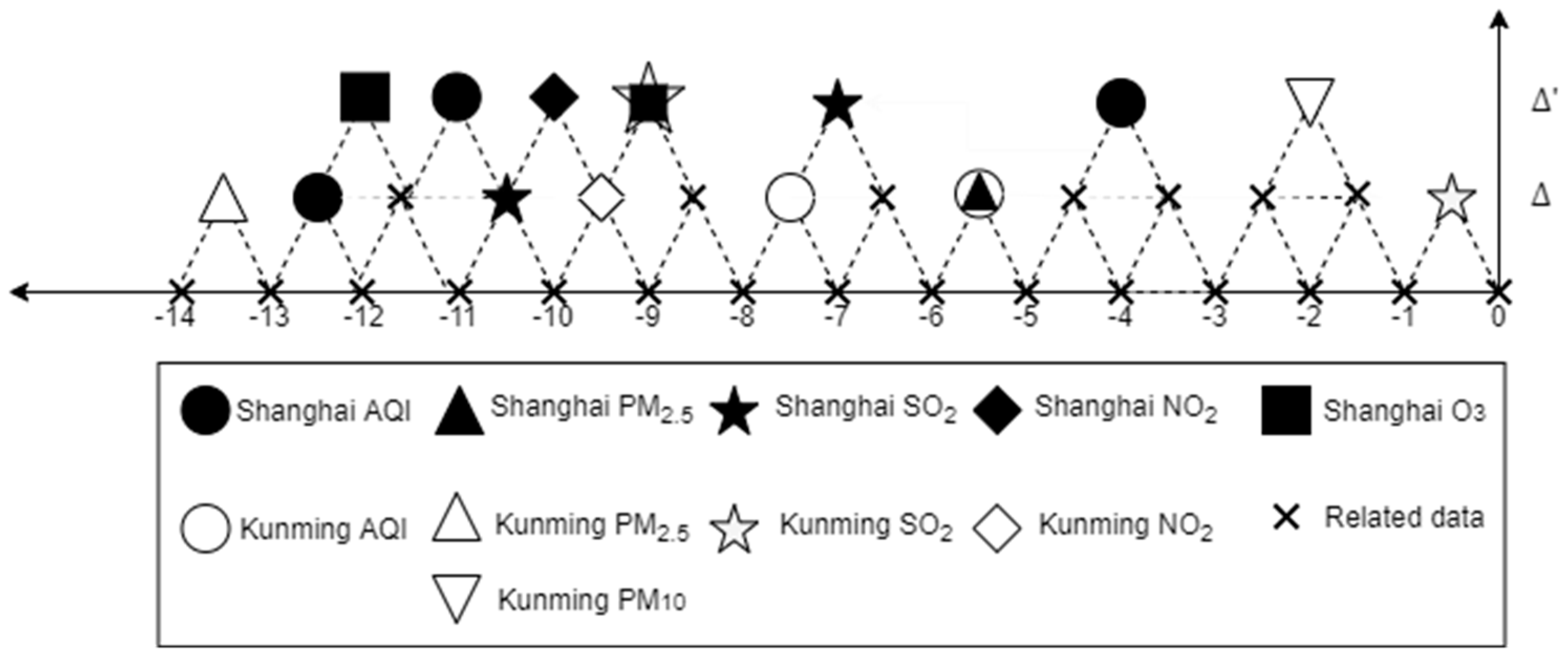
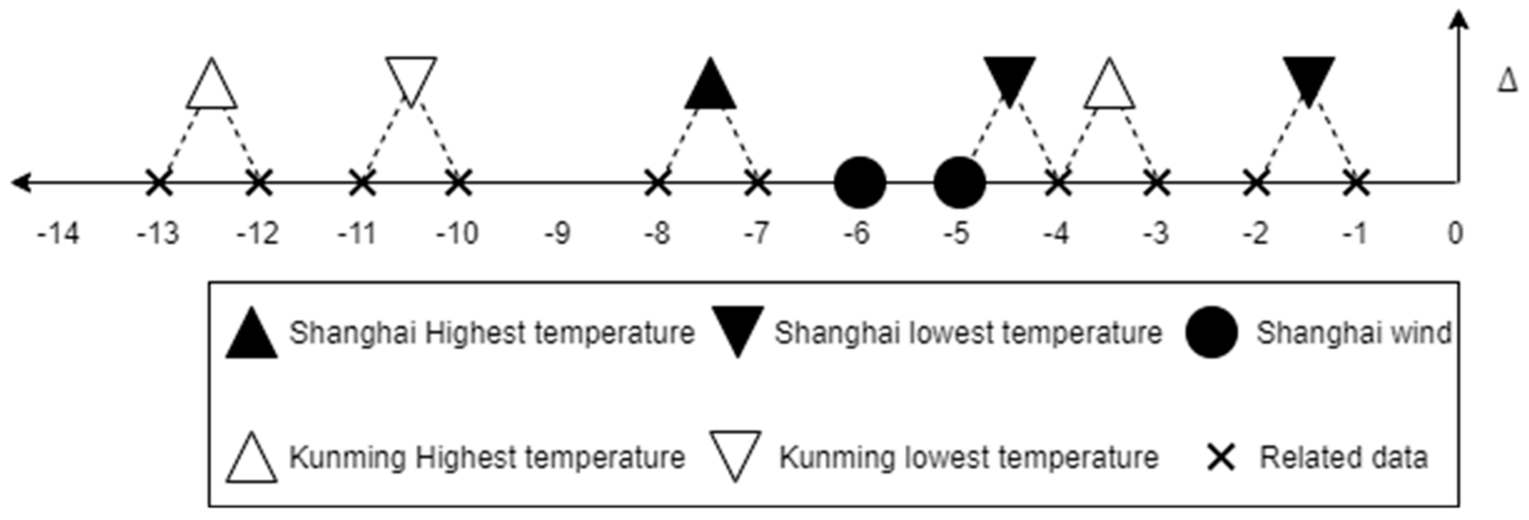
3.1. Data Collection and Resources

Shanghai MicroPort Medical (Group) Co., Ltd. (Shanghai, China) provided the research data containing the participants’ test location, test time (date), and their health statuses (whether at a high risk of AF). All the data were collected through the investigation, and there was no private data of the participants. What is more, the duration of the investigations in Shanghai and Kunming were 1 year and 6 months, respectively. In addition, the related environmental factors were provided, including the current day and the previous 14 days’ weather, temperature (with the unit of degrees Celsius), wind force scales, air quality indexes (AQI), and air pollution concentrations (PM2.5, PM10, NO2, SO2, O3, CO), where the first five kinds of pollutants used the unit of µg/m3, except for CO, with the unit of mg/m3. Therefore, there are 11 independent variables for each day, 15 days involved, and the AF status is the dependent variable.
In this research, two databases of Kunming and Shanghai were used to analyze the impact of the air pollution issue and the effect of other environmental factors. There were 3518 records collected, and after removing the incomplete records, 3160 records were kept (732 for Shanghai and 2428 for Kunming, respectively). Meanwhile, the high-risk AF (ICD-10 code I48) rate for Shanghai and Kunming participants were 9.3% and 2.8%, respectively. This research divided the data into two parts based on the AF status, as modeling parts (80%) and checking parts (20%), according to the locations.

3.2. Research Logic and Data Curation

This paper establishes a two-step analysis process, and the variables are categorized into five types. The first step is to convert the parameters into binary variables and analyze whether they are significantly related to AF or not. The second step is to use the primary data to establish a logistic regression model to interrupt the effect quantitatively.
In the first step, every related factors’ differences were calculated to demonstrate the changes between the following days, shown in Equation 1 below.
Δ ( X ) j , t i , B = { 1 when ( X ) j , t i ( X ) j , t + 1 i > 0 0 when ( X ) j , t i ( X ) j , t + 1 i 0
where Δ ( X ) j , t i , B is a binary variable recording the increase or decrease of the variable X between the day t and a day before for participant i , for which 1 means an increase and 0 means a decrease or equal. ( X ) j , t i denotes the value of the factor X on the day t for the tester i in city j . For instance, ( AQI ) 5 i represents the AQI index for the participant i on the day (5 days before the test day). Hence, if the Δ ( X ) j , t i , B is positive, it means that the environment is getting worse from day t + 1 to day t.
In this research, all Δ ( X ) j , t i , B are classified into the first-order difference category. What is more, to denote AF’s situation, this paper use 1 to represent the patient being at a high risk of AF (over 50% chance of AF), and 0 for low risk (less than 50%). Furthermore, this research calculates the second-order differences, categorized into the second-order-difference type, to illustrate the fluctuating rate, shown in Equation (2) below.
Δ ( X ) j , t i , B = { 1 when Δ ( X ) j , t 1 i Δ ( X ) j , t i > 0 0 when Δ ( X ) j , t 1 i Δ ( X ) j , t i 0
where Δ ( X ) j , t i , B denotes whether the fluctuating speed of the difference of variable X between the day t − 1 and t and the difference between the day t and t + 1 for the participant i in city j . Based on the definition of the second-order-difference variables, if the value is zero, it means that the change is stable, keeping an unchanging tendency. However, if it is positive, it could represent one of the following three situations: (1) the value’s decreasing rate is getting lower. (2) The value’s increasing speed is getting faster. (3) ( X ) j , t i is the smallest compared with ( X ) j , t 1 i and ( X ) j , t + 1 i . To sum up, if the second-order-difference variable is positive, it describes a more complicated environmental degradation.
Therefore, there are 384 variables in this two-step research, divided into five categories (AF, primary pollution indexes, temperature, weather, and wind scale, first-order difference, and second-order difference, respectively). This research uses SPSS software (International Business Machines Corporation. Armonk, NY, USA. Version 25) to analyze the association between environmental factors and the incidence of AF and establish binary logistic models to elaborate on the relationship.
In the first step, all differences of variables (first-order difference and second-order difference) were converted into binary variables for modeling, 1 denoting the increase and 0 for the decrease.

3.3. Binary Logistic Regression

This research established two models through binary logistic regression, one for Shanghai and one for Kunming (called model 1 and model 2). Many scholars have used this method to determine the association between the risk factors and CVD [31,32,33], while this research concentrates on the changing of environmental factors. With the binary logistic regression, this research established the models as:
p j i = e ( c + D j i + U j , 0 i + U j , 1 i + U j , 2 i ) 1 + e ( c + D j , 0 i + U j , 0 i + U j , 1 i + U j , 2 i )
U j , 0 i = t β X , t j , 0 × ( X ) j , t i
U j , 1 i = t β X , t j , 1 × Δ ( X ) j , t i
U j , 2 i = t β X , t j , 2 × Δ ( X ) j , t i
D j i = { 0       if ( X ) j , t i = 0 d , l β d , t l       if ( X ) j , t i = 1
where p j i denotes the probability that participant i has a high risk of AF, and U j , 0 i , U j , 1 i , and U j , 2 i represents the utility of the sum of the primary factors (except for weather and wind scale), and the utilities of the sum of the first-order category factors and the second-order category factors, respectively. D j i is the sum of the dummy variables, representing the different situations of the weather and wind scales. β X , t j , 2 is the coefficients of the factor X in location j (Shanghai or Kunming, or the composition of the two cities) of the difference calculating order n (0 or 1 or 2) of the time t . Using the binary variables and the primary value of the factors, the p j i value could be calculated.
With 95% confidence interval (95% CI), this research first selected the statistically significant variables by checking their Wald statistic. What is more, this research reconsidered the correlations between every two variables to optimize the models.
With the binary logistic model results, the effect of the factors could be estimated by the coefficients’ value. Besides, the odds ratio (OR) values were calculated to demonstrate the factors’ impact, which equaled the exponential of β X , t j , n . If the OR value was larger than 1, it represented the specific factor’s increase, positively related to the increase of the AF risk.

3.4. Model Tests

In this part, the models were tested by three methods, including chi-square tests, receiver operating characteristic curve (ROC curve) plotting, and applying to the new data sample to check the accuracy.
This research firstly analyzed the models’ goodness of fit via omnibus tests and the Hosmer and Lemeshow test. They both use the chi-square value to check whether the model is further optimized to reject the null hypothesis. By comparing the chi-square values and the related p-values, it is persuasive to reject the null hypothesis evidently. Moreover, as many scholars have used the ROC-AUC approach in this field [34,35,36,37], this research used this method to examine this model’s accuracy.
In conclusion, this research firstly checked the significance of all the variables and then used four methods to determine the models’ statistical significance to determine the association between environmental factors and AF.

4. Results

This research establishes two models through the analysis methods above, and they could show three vital results about the environmental factors to AF, from the epidemical, geographical, and lag-affect pattern aspects.

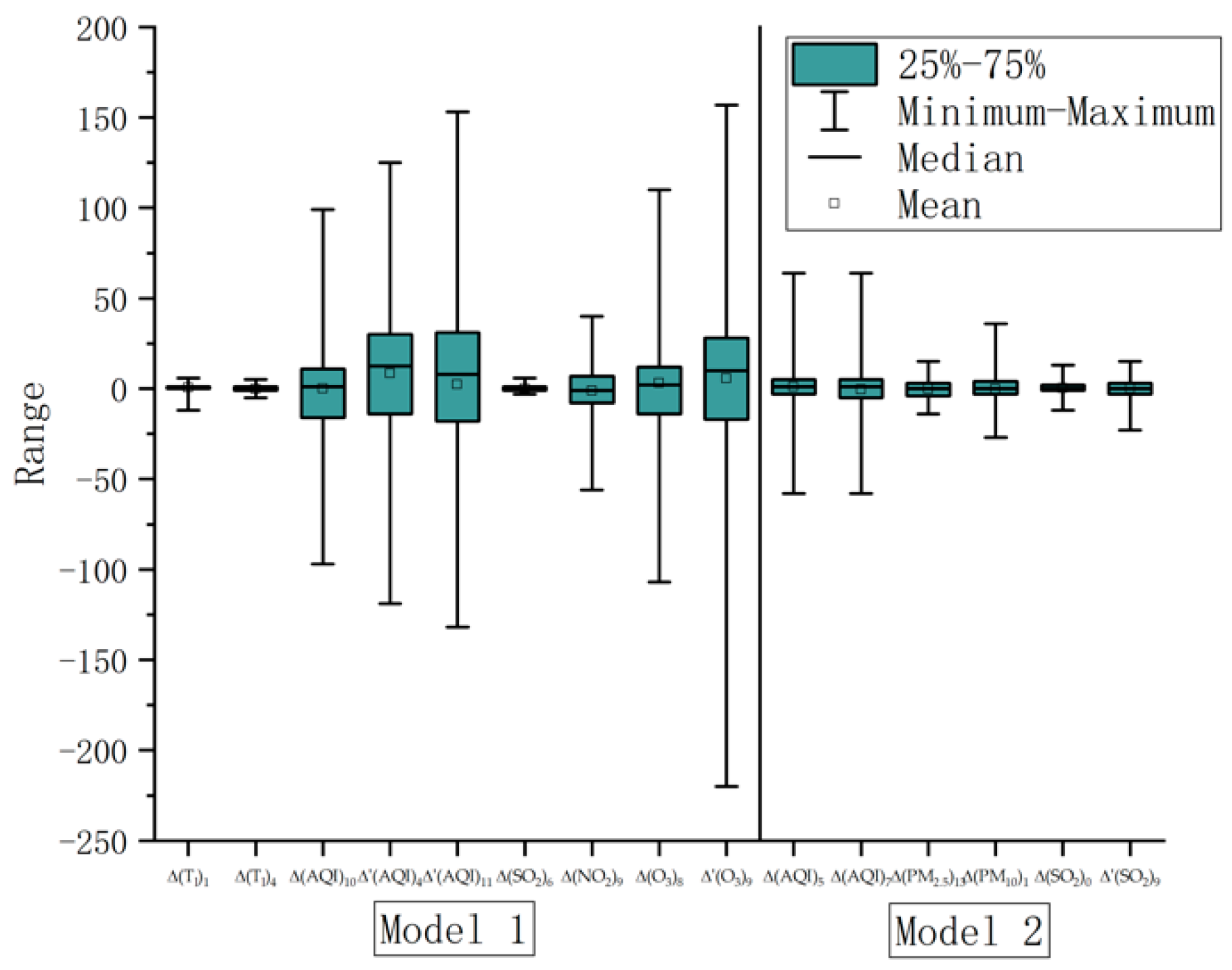
4.1. Qualitative Models’ Results

Analyzing the data using SPSS, this research figured out the factors that significantly affect the AF status qualitatively as the first step to establishing the models. The result is shown in Figure 1 and Figure 2 (the qualitative model is in the Appendix A in Table A1).
As mentioned above, the Δ and Δ′ in the two figures above denote the first and second-time differences. This step is used to figure out the significant factors and the related variables.

4.2. Quantitative Models Results

Using SPSS 25, the following two models in Table 1 below exhibit the quantitative relationship between the specific environmental factors and AF.
In the tables above, the OR value is the impact of per 1 unit increase of the particular variable on AF’s incidence when other conditions are all kept unchanged, which equals to the exp(β). The following Figure 3 and Figure 4 plot the OR values with their lower and upper bounds, where the Y-axis shows the variables and the X-axis shows the corresponding OR values range with 95% CI and the expected OR value.
For example, the Δ(SO2)6 in Table 1 model 1 is 1.508 (95% CI: 1.168, 1.947), larger than 1, showing that, with all other variables kept the same, for every 1 unit increase of the SO2 index from the seventh day before the test date to the sixth day, the risk would increase by 1.508 times. In contrast, for the (Th)3 (OR value as 0.813) in model 2, if the highest temperature occurred on the third day before the record increasing 1 degree, the patients in Kunming would have a lower probability of getting AF on the testing day, and the probability would decrease by about 20%. Therefore, the models’ results could illustrate the relationship between environmental conditions changing and AF risk changing. What is more, with the descriptive statistics, the absolute value of the variables and related variables could be illustrated, showing the results more detailed and evidently.
As air pollution could last for days, and the air quality tendency is ordinarily stable in a particular city, the correlation between variables in this research is appropriately released. Hence, some variables may still be kept for the accuracy of the models. Moreover, by analyzing the data of air quality, wind scale, and temperature to assist in analyzing the association, this research used Figure 5 and Figure 6 to illustrate the value of those selected variables. In the two figures, the boxes to the left of the vertical lines are for model 1, and others for model 2, and they describe the upper and lower bound of the value of the factors with their 25% to 75% range. The spots and the horizontal lines inside the boxes denote the mean and median values, respectively.
As most coefficients in the two models were from −1 to 1, with a larger value of the variable, this specific factor would cause a more significant impact. For instance, the (O3)8 in model 1 is statistically significant, and the mean and median value of this variable were close to 100, larger than other factors’; therefore, the impact of the concentration of O3 (lag of 8 days) could be evidently shown. Besides, judging by this graph, some insignificant variables could be explained, for example, Δ(PM10)1 in model 2 (p-value is 0.602). In Figure 6, it is clear that the variable’s value was close to 0, and half of them distributed close to 0. Therefore, the impact given by PM10’s concentration changing was limited. Hence, compared with other factors, it could be statistically insignificant. In conclusion, these two figures above can explain the models’ results by analyzing the distribution and value of the variables.
What is more, many variables were insignificant in the models because they could explain the first step’s results. For example, the second-difference AQI value of four days before the test day in Shanghai (denoted as Δ′ (AQI)4) was insignificant, with 95% CI (p-value as 0.089), which is kept to show the impact of the AQI changing from the fifth day to the third day before the test day, which was found significant in the first step. Other insignificant variables played the same role. Besides, all insignificant variables’ OR interval skipped 1, so it is hard to identify them to judge their impact confidently. Nevertheless, those variables are vital to support the conclusion achieved in the first step.
According to the tests of the models, the results of the goodness of fit test results are shown in Table 2. With the omnibus test’s chi-square values and the significance values of all passing the test, it is evident that we can judge that the models are eloquent. As the p-values for the omnibus tests are all less than 0.5, this represents that the null hypothesis test could be rejected. Besides, the Hosmer and Lemeshow test results show that the information of the data has been fully extracted (all p-values are larger than 0.05), which means the models have good fitness. Therefore, from the results of these two tests of the models, all models have been proven to be relatively accurate.
The ROC-AUC test results are shown in Table 3 below. As the AUC represents the degree or measure of separability of the model, it was chosen to be an approach to analyze the models’ accuracy. Therefore, taking the AUC value for Shanghai’s model as an example, which is 0.824 (95% CI: 0.771, 0.877), it represents excellent discrimination. Besides, the AUC value for model 2 is 0.756, denoting that the model is acceptable and has excellent abilities to separate AF’s risk level.
Furthermore, by calculating the accuracy by checking the sample data, the accuracy was 88.8% and 97.3% for the two models mentioned above. As this research focused on the association between environmental factors and AF prevalence, the accuracy could prove the models’ validity.
In conclusion, all models have shown great accuracy, separability, and information extraction through these three tests’ results. Hence, these models were selected to analyze the association between AF and environmental factors.

4.3. Epidemicical Results

The epidemical result is that three of the most common air pollutants mentioned by the WHO were positively correlated with the prevalence of AF, as PM, NO2, and SO2. Moreover, as the AQI is a synthetic factor in measuring the pollution level, the OR values of the AQI could demonstrate the impact of air pollution comprehensively.
Judging by the models, it is clear that with PM and SO2 concentration increasing, it poses a higher risk for people getting AF, proven by the OR value of the concentration increase of PM2.5 13 days prior to the test day in Kunming (95% CI: 1.062, 1.208) and SO2 6 days prior in Shanghai (95% CI: 1.168, 1.947), respectively. Moreover, model 1 highlights that the concentration of O3 had a negative impact, which was proven by the OR value for the O3 concentration per 1 unit increase in fluctuation around the ninth day before the record date (95% CI: 1.000, 1.034). What is more, the AQI’s increase 5 days (95% CI: 1.019, 1.066) and 7 days (95% CI: 1.003, 1.056) previously in model 2 prove that the comprehensive air pollution increase will cause the patients to get into a more dangerous environment.
Concentrating on the fluctuation of air pollutant concentrations (defined by the second-order difference category), all coefficients were positive, except for one, the AQI fluctuation 11 days before the test day in model 1. However, by analyzing the primary data, it shows that the AQI index from the 12 days prior to the 10 days before the test day followed the increasing trend, while the increasing speed slowed down. Therefore, this research concludes that if the air pollution situation shows the tendency of going down initially and then immediately going up, there will be a higher risk of AF.
This paper uses the following Figure 7 and Figure 8 to illustrate the impact of the pollutants and temperature changes.
The X-axis value is the odds change value, representing the changing of AF’s incidence when the specific variable increases by 1 unit. From the two figures shown above, it is clear that different cities are sensitive to different parameters. What is more, SO2 is more significant than the other variables, not only because the odds change is larger than for the others (close to 0.5), but also because both models contain this pollutant. Besides, as shown in Figure 7 and Figure 8, it is clear that with the pollution getting severe, regardless of the absolute index or the polluting speeding up, people will have a higher risk of AF. For instance, the probability of AF for patients in Kunming will have 4% increase if there is 1 unit increase of the AQI, since from the sixth day to the fifth before the test day. The SO2 increase 1 day previously played a protective role, because, in Kunming, the SO2 concentration was relatively stable (mean and standard error for the increase is 0.21 and 0.057); if the concentration increases significantly, the impact could be significant.
Finally, both models’ constant coefficients were negative, as a protecting factor from AF. There are few high-risk patients in the database (67 in Kunming and 68 in Shanghai) compared to low-risk people through the statistical analysis. Therefore, the constants here demonstrate that only a few people are at high risk in the initial stage.
To sum up, from the results related to the pollutants’ concentrations, it is clear that air pollution may cause the prevalence of AF growth. Similarly, the second-order difference demonstrates that the fluctuating rate of the air pollutants’ concentrations changing can significantly affect AF prevalence.

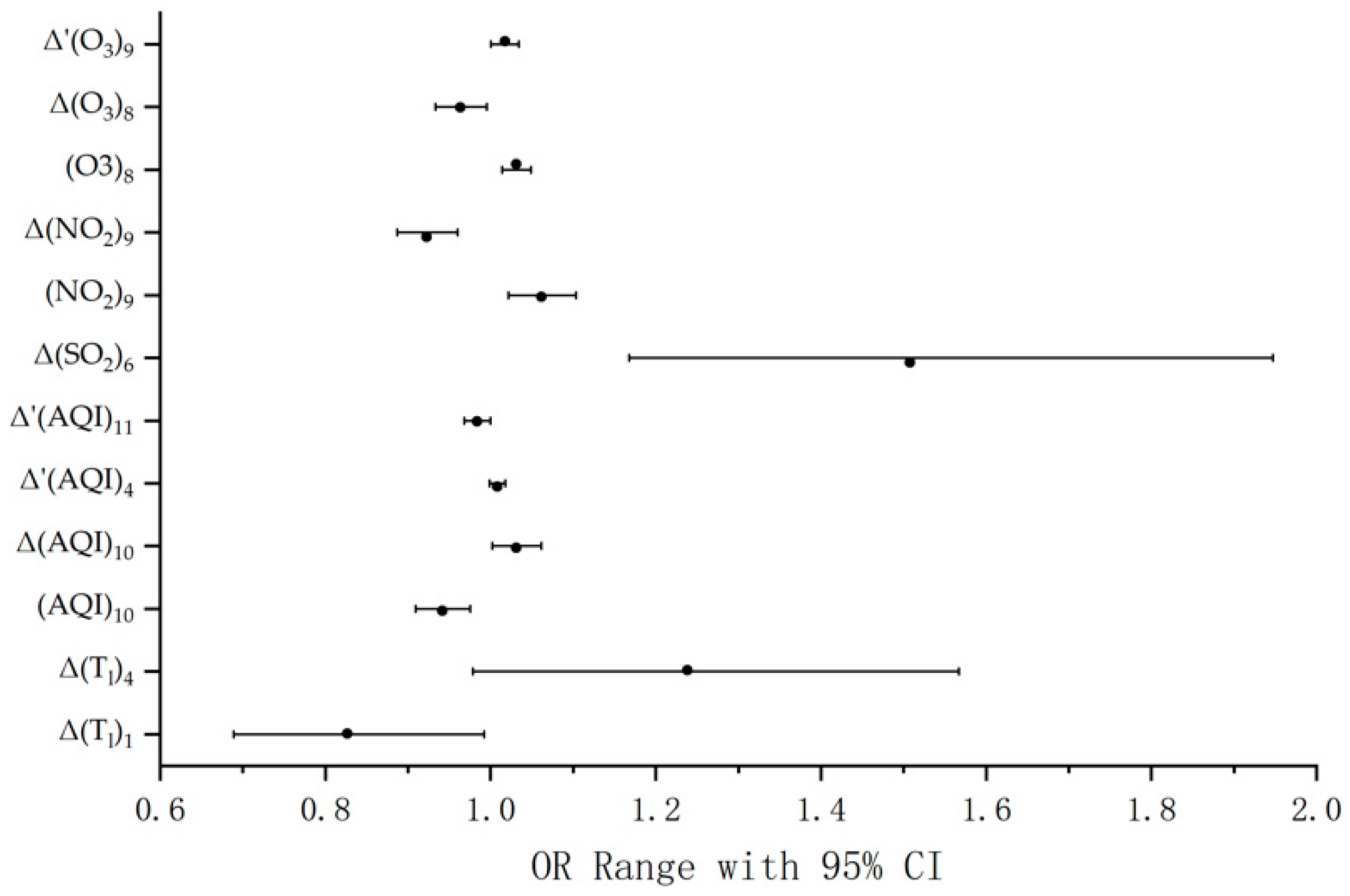
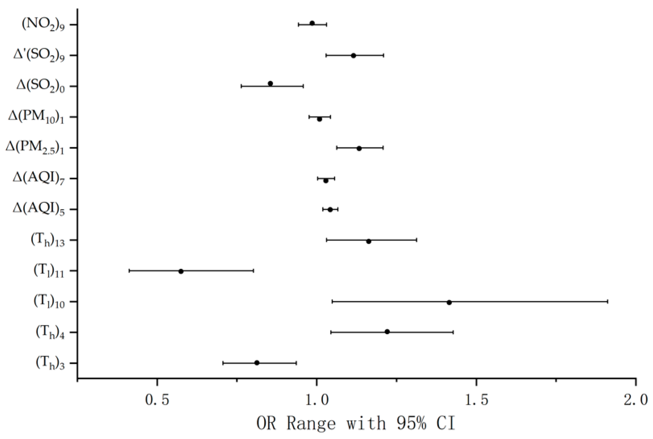
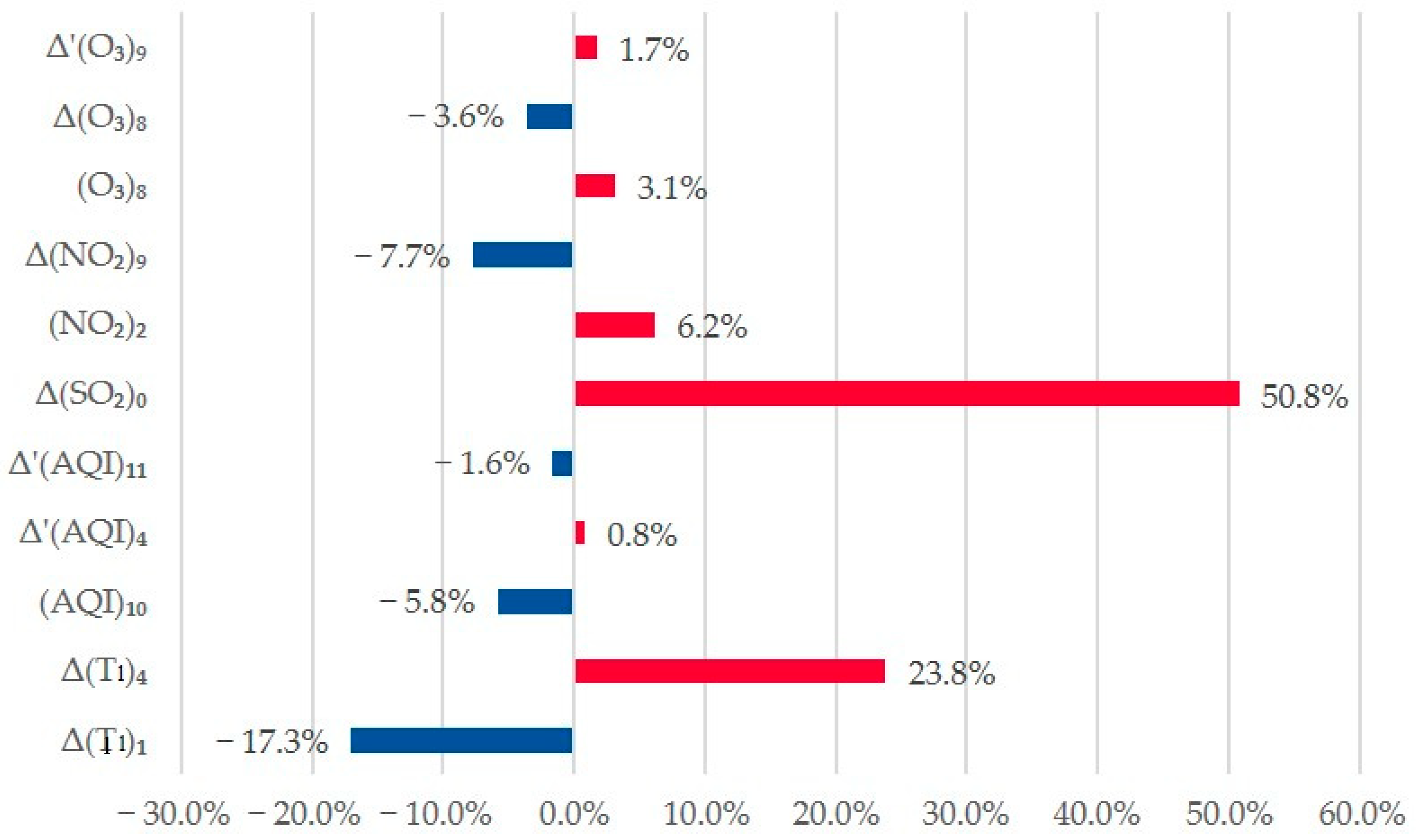
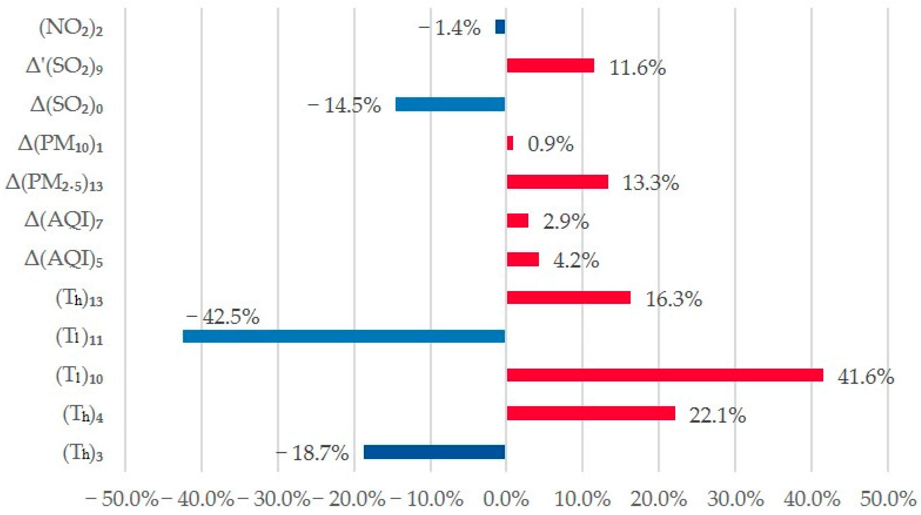
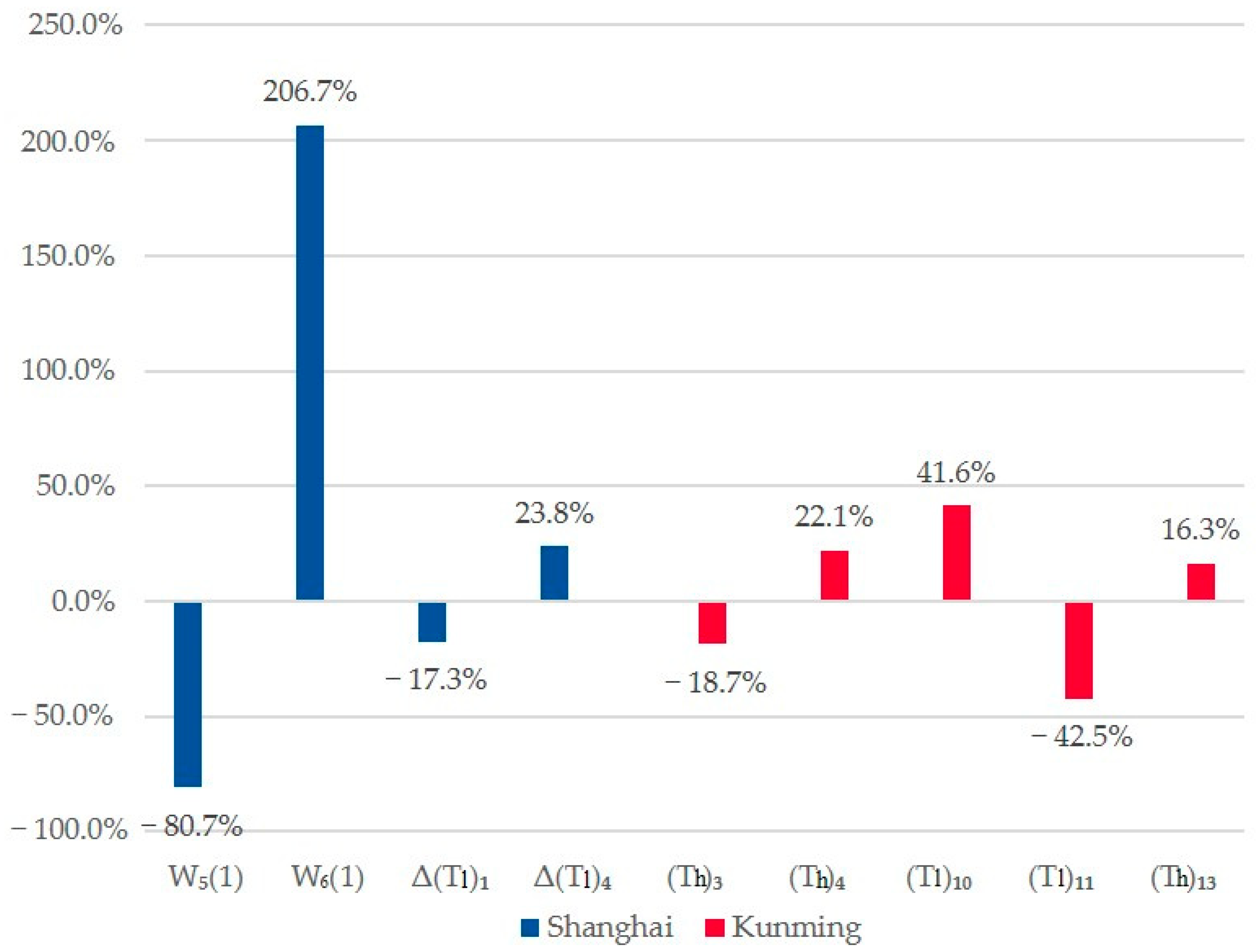
4.4. Geographical Results

The geographical effect is clear from the models, mainly represented by the model variables involved. According to model 1 and model 2, it is clear that they contain different variables. The following Figure 9 illustrates the comparisons of the odds change of the temperature and wind on AF.
Nevertheless, different cities are sensitive to different days. From Figure 9, the AF incidence in Shanghai was not sensitive to the temperature, while it was closely related to the weather. In contrast, the situation in Kunming was the opposite. The OR values of the lowest temperature that occurred in Kunming (10 and 11 days lag for Kunming) were 1.416 (95% CI: 1.048, 1.911) and 0.575 (95% CI: 0.412, 0.802), showing that the different days’ temperature had a different impact. Although the temperature was usually kept at a relatively stable level, the impacts may have offset each other, and may have caused a considerable effect when the temperatures were changing a lot during those days.
Concentrating on the wind scales’ impacts, it had a relatively complex influence. If the wind scale was above level 4 on the sixth day before the test, people had a higher probability of getting AF (95% CI: 1.330, 7.076) in Shanghai, while the wind on the five days lag decreased the chance (95% CI: 0.054, 0.689).
In conclusion, the models describe the difference caused by the location of the patients. The impact of geography is entire, while the negative impact of air pollution is the same.

4.5. Pollution’s Lag-Pattern Impact

In this research, most of the variables were not directly related to the test date, with a lag of 3 to 12 days. Therefore, it is reasonable to conclude that the risk of AF is associated with the environment and air pollutions. Comparing the models, nearly all the significant variables had at least three days lag, representing that the impact of the pollution could not immediately cause AF.

5. Discussion

5.1. The Influence of Air Pollution Factors on AF

There has been some research concentrating on the medical mechanism of the impact given by environmental factors on CVD. For example, Bhatnagar [38] in 2004 asserted that, as important components of PM2.5, metals in the environment deposit in the heart and blood vessels, and their toxicity increases the risk of CVD. Besides, some gaseous pollutants can mediate or modify PM, which may cause ischemic heart diseases. Similarly, it has been proven that O3 is highly related to pulmonary inflammation and edema, but it is still unclear whether it is associated with CVD [39]. Besides, other research figured out that environmental factors (especially air pollution) can cause CVD, such as endothelial dysfunction and the role of oxidative stress [40], which proves this paper’s results. What is more, PM can cause atherosclerosis via promoting vascular dysfunction and alternating the vasoactive mediators’ responsiveness [41]. These results explain the medical mechanism of CVD related to environmental factors, and they highlight the significant impact of environmental factors, which shows the importance of this paper’s research.
After adjusting for other gaseous pollutants, the significance of PM2.5, PM10, SO2, NO2, and O3 in research results is highlighted, suggesting that they are currently the main pollutants in Shanghai and Kunming. There is a positive correlation between the risk of AF for people in Shanghai and Kunming and the increase in PM concentration [42]. Other studies have evaluated the impact of six major environmental pollutants on the risk of AF in patients with cardiac implantable electronic devices (CIED). With a 10 μg/m3 increase in PM2.5 and PM10 concentrations, the risk of AF increased by 3.8% and 2.7%, respectively; however, the correlation with other gaseous pollutants (SO2, NO2, CO, O3) was not statistically significant [43,44], which is similar to this research’s results. Furthermore, this research emphasizes the impact of air pollution fluctuations in Shanghai and Kunming, filling the blanks of previous research.
On the other hand, statistics show that the increase in the number of visits for arrhythmia in the emergency room was significantly related to PM2.5 on warm days (>23 °C) and cold days (<23 °C), and high levels of PM2.5 would increase the risk of emergency visits due to arrhythmia [45]. In this research, the average highest temperature in Shanghai on the seventh and eighth day before was 23.3 °C, and 22.8 °C (standard error as 0.334 °C and 0.312 °C), respectively, and the lowest temperature in Kunming was close to 23 °C as well, which meets the conclusion. A large number of studies have explained this impact from the perspective of pathology, as certain substances can cause oxidative stress, cardiovascular inflammation, endothelial dysfunction, high C-reactive protein level, myocardial ischemia, and right atrial pressure [46,47,48,49,50], all of which are related to atrial remodeling and AF pathophysiology [51,52,53,54].
Therefore, it is persuasive to confirm that air pollution has the risk of increasing the probability of arrhythmia or other acute cardiac events. Hence, patients at high risk of AF should be educated to monitor the local air quality index and follow the recommendations to reduce exposure and reduce outdoor activities. What is more, this research helps prevent AF’s high-risk situation and can give an early warning to the number of outpatients increasing through the lag-affect analysis of air pollution and wind. Therefore, this research can further strengthen the theoretical basis of urban air pollution control, establish air pollution control measures, and optimize community and hospital diagnoses and treatment configuration.

5.2. AF Risk Factors Are Variable in Different Cities

According to this research, for the results of model 1 and model 2, air pollution particles’ impact on AF incidence was similar, while the impact of temperature factors showed opposite laws. Besides, the risk of AF in Shanghai was more sensitive to the effects wind scale, while that in Kunming was not.
Many studies have shown that the effects of seasons and temperature on the incidence and mortality of cardiovascular diseases are different in different cities [55,56]. The results of an epidemiological study containing 16 cities in China showed that PM10 was significantly associated with deaths from cardiopulmonary system diseases, and the association is still statistically significant after adjusting for other gaseous pollutants; additionally, the relationship between PM10 and death risk in different cities differed due to the different levels of pollutants in each city [57]. It explains the reason why the impact of PM10’s concentration increase has different lag periods.
The seasons’ effect on the risk of AF is another consideration. K Spengos et al. analyzed the symptom onset pattern of more than 300 patients with acute cardiogenic stroke in Greece for the first time due to AF, figuring out that the patients’ symptoms were cyclically distributed, with the peak season in winter and the incidence in summer declining [58]. Similarly, J Ahn et al.’s study of the seasonal changes in AF incidence in Seoul also showed that the frequency of AF in summer was significantly lower than in other seasons [59]. Moreover, a national statistical study in Germany showed that when the outdoor temperature was between 0 and 10 °C, the hospital admission rate for arrhythmia, including AF, reached its peak [60]; however, some studies have shown that in some temperate countries, cardiovascular diseases in winter are lower than in summer [61]. Although most participants took the test in autumn in this research, it is hard to show the seasonal impact, and the different impacts of changing temperature, weather, and wind scale on AF risk have been pointed out.
In summary, different cities have different effects on the incidence of AF due to the intensity, mode of action, duration of the effect of cold and heat, and maybe the local residents’ physical fitness. Therefore, different locations may have their own specific models to estimate the risk of AF, which might be another way to describe whether a city is livable or not.

5.3. The Impact’s Lag-Affect Pattern

The lag-effect of environmental factors’ impact on AF is shown by the variables’ OR values, most of which show a three to twelve days lag. For example, the increase of the previous six day’s SO2’s concentration is statistically significant in Shanghai. Although the four kinds of air pollutants (PM2.5, PM10, SO2, and O3) could significantly affect AF incidence, they all show lag-affect influence.
Many studies have also confirmed that the lag of air pollutants may affect the occurrence of CVD and the mortality rate. The correlation between PM2.5 and CVD mortality mainly occurred in the first 6 days, with the fourth day being the most significant [62]. Additionally, LC Martins and other scholars have asserted that air pollutants’ delayed effects (CO, PM10, O3, NO2, and SO2) have different effects on different genders. Besides heart failure inducing diseases, the delayed effects have more noticeable effects on women for other cardiovascular diseases [63]. Similarly, M Dastoorpoor et al. announced that for people over age 60 and under 18, after a delay of 3 days and 13 days, there was also a significant relationship between the increase in the interquartile range (IQR) of particles below 10 μm and cardiovascular death. For those under 18 years old (lag 11) and over 60 years old (lag 9), there was a significant relationship between the increase in IQR of NO2 and CO and cardiovascular death, respectively [64]. Kim et al. pointed out that the number of lag days for the impact of PM2.5 on CVD depended on its chemical composition, and the different lag times may vary with the patient’s health status and disease [65].
This research selected the medical records in Shanghai and Kunming for statistical research, and the conclusion showed the similarity with the previous study. Notably, the pollutants’ delayed impact on AF in the two cities was different, which may be due to the study cities’ different characteristics, such as indoor air quality, local climate type, residents’ sensitivity to pollutants (such as economic level, population age, and smoking rate), pollutant concentration levels, and differences in pollutant composition.

5.4. Research Significance, Limitations and Prospects

This research attempted to figure out the association between environmental factors and AF, which is of significance to the government, medical research, and patients. As it emphasizes the hysteresis of air pollutions and weather changes’ impact, the government and hospitals can use these conclusions to improve and optimize weather reports and forecasting. Meanwhile, this research uses the data of two cities in China, comparing and demonstrating the different impacts caused by the different locations. Therefore, other researchers can follow this direction to determine the overall regularity, boosting AF and CVD comprehension. Furthermore, patients with a history of AF could be alerted by this research to pay more attention to air pollution and take self-protection more seriously. On the other hand, medical workers may also remind the patients to remember the air pollution conditions in order to protect them in the following days.
However, there were still some limitations to this research. This research used the average value of each monitoring site in each city as the population exposure level of pollutants. However, each monitoring site’s pollutant measurement methods may differ, so the environmental monitoring results and the individual level of pollutant exposure might not be accurate enough. Hence, this study cannot calculate the precise individual exposure in each city, affecting the analysis results. Meanwhile, as the participants’ gender and age level were often misrecorded in the records, this research does not contain those two vital factors to optimize the model. What is more, as most of the data were collected in the summer and autumn, some contingents might exist in this paper’s results. Therefore, more data are being collected by a more extended duration investigation and tracking surveys, which can help to improve the results. In the subsequent research, more detailed data will be used to optimize the models and provide more conclusions.

6. Conclusions

Increasing environmental pollution will increase the incidence of atrial fibrillation, and the concentration of the increase of the two major air pollutants (PM10 and SO2) will raise the risk significantly. Meanwhile, the environmental impact of each region is regional and lagging. Besides, the acceleration of air pollution will also increase the probability of atrial fibrillation. Therefore, continuously monitoring the environmental indexes are of importance for warning and protecting potential patients. What is more, different cities may have their unique model to evaluate and estimate the significant factors to improve the local environmental departments’ working process, as integrating the previous environmental indexes into the daily weather reports has a strong impact on the sustainability of AF.

Author Contributions

Conceptualization, S.L. and Y.Z.; resources, S.L., Q.Z., and W.Y.; investigation, S.L.; data curation, Y.Z.; formal analysis, S.L. and Y.Z.; methodology, Y.Z.; software, Y.Z. and Q.Z.; project administration, S.L.; writing—original draft, Z.C. and M.D.; writing—review and editing, Y.Z., Z.C., M.D, and W.Y.; validation, Q.Z. and W.Y. All authors have read and agreed to the published version of the manuscript.

Funding

This work is financially supported by Shanghai Key Laboratory of Interventional Medical Devices and Equipment (NO. 19DZ2230500), the National and Regional Research Projects of Ministry of Education of the People’s Republic of China in 2020 (2020-N53), the Decision Consulting Cultivation Project of University of Shanghai for Science and Technology (2020-JCPY-01), and the Connotation Construction Project for University Think Tank of Shanghai Municipal Education Commission (20ZKNH068).

Institutional Review Board Statement

Not applicable.

Informed Consent Statement

Not applicable.

Data Availability Statement

The data presented in this study are all from the statistical data officially released by China and have been explained in the text and references.

Acknowledgments

This research is technically supported by Yang Cuiwei, professor of the Department of Electronic Engineering, Fudan University.

Conflicts of Interest

We have no conflict of interest to declare. All the authors have seen and approved the manuscript being submitted.

Appendix A

Table A1. The qualitative model results.
DescriptionVariablesShanghaiKunming
β 1Std. 2Sig. 3OROR 4 95% CIβStd.Sig.OROR 4 95% CI
Lower BoundUpper BoundLower BoundUpper Bound
WindW5(1)−2.9000.7600.0000.0550.0120.244
W6(1)2.4980.5520.00012.1624.11935.917
TemperatureΔ(Tl)1−1.2130.4390.0060.2970.1260.703
Δ(Tl)41.9990.4550.0007.3783.02218.013
(Th)71.6620.4540.0005.2672.16212.833
Δ(Th)3 −0.9060.3700.0140.4040.1960.835
Δ(Tl)101.0950.3360.0012.9881.5455.777
Δ(Th)12−1.9830.5410.0000.1380.0480.397
AQIΔ(AQI)5 0.7630.3090.0142.1441.1703.928
Δ(AQI)7−1.1050.3460.0010.3310.1680.652
Δ(AQI)12−1.8570.4530.0000.1560.0640.379
Δ′(AQI)41.9350.4450.0006.9252.89316.578
Δ′(AQI)11−1.8340.4770.0000.1600.0630.407
TSPΔ(PM2.5)50.9260.4220.0282.5251.1055.770
Δ(PM2.5)13 0.8270.3160.0092.2851.2304.246
Δ′(PM10)20.7700.3450.0262.1601.0984.248
SO2Δ(SO2)0 −1.1560.3720.0020.3150.1520.652
Δ(SO2)101.3050.4240.0023.6861.6068.457
Δ′(SO2)71.9600.4160.0007.1023.14216.056
Δ′(SO2)9 0.7630.3450.0272.1451.0914.218
NO2Δ(NO2)9 −1.2640.3490.0000.2830.1430.560
Δ′(NO2)10−1.4190.4300.0010.2420.1040.562
O3Δ′(O3)90.9130.4250.0322.4911.0835.726
Δ′(O3)12−1.3630.4370.0020.2560.1090.603
Constantc−4.2220.8540.0000.015 −3.7730.5790.0000.023
1 The β in this table represents the coefficients of the variables. 2 The Std. in this table represents the coefficients’ standard deviation value. 3 The sig. in this table denotes the p-value of the variables. 4 The OR in this table denotes the odds ratio value.

References

  1. Camm, A.J.; Kirchhof, P.; Lip, G.Y.H.; Schotten, U.; Savelieva, I.; Ernst, S.; Van Gelder, I.C.; Al Attar, N.; Hindricks, G.; Prendergast, B.; et al. Guidelines for the management of atrial fibrillation: The Task Force for the Management of Atrial Fibrillation of the European Society of Cardiology (ESC). Eur. Heart J. 2010, 31, 2369–2429. [Google Scholar]
  2. Guo, Y.; Tian, Y.; Wang, H.; Si, Q.; Wang, Y.; Lip, G.Y.H. Prevalence, incidence, and lifetime risk of atrial fibrillation in China: New insights into the global burden of atrial fibrillation. Chest 2015, 147, 109–119. [Google Scholar] [CrossRef]
  3. Wang, Z.; Chen, Z.; Wang, X.; Zhang, L.; Li, S.; Tian, Y.; Shao, L.; Hu, H.; Gao, R. The Disease Burden of Atrial Fibrillation in China from a National Cross-sectional Survey. Am. J. Cardiol. 2018, 122, 793–798. [Google Scholar] [CrossRef] [PubMed]
  4. Zhou, Z.; Hu, D. An epidemiological study on the prevalence of atrial fibrillation in the Chinese population of mainland China. J. Epidemiol. 2008, 18, 209–216. [Google Scholar] [CrossRef] [PubMed] [Green Version]
  5. Friberg, L.; Rosenqvist, M.; Lip, G.Y.H. Evaluation of risk stratification schemes for ischaemic stroke and bleeding in 182 678 patients with atrial fibrillation: The Swedish Atrial Fibrillation cohort study. Eur. Heart J. 2012, 33, 1500–1510. [Google Scholar] [CrossRef]
  6. Gao, H.; Yang, W.; Wang, J.; Zheng, X. Analysis of the Effectiveness of Air Pollution Control Policies based on Historical Evaluation and Deep Learning Forecast: A Case Study of Chengdu-Chongqing Region in China. Sustainability 2021, 13, 206. [Google Scholar] [CrossRef]
  7. Liu, H.; Liu, J.; Yang, W.; Chen, J.; Zhu, M. Analysis and Prediction of Land Use in Beijing-Tianjin-Hebei Region: A Study Based on the Improved Convolutional Neural Network Model. Sustainability 2020, 12, 3002. [Google Scholar] [CrossRef] [Green Version]
  8. Andrew, N.E.; Thrift, A.G.; Cadilhac, D.A. The prevalence, impact and economic implications of atrial fibrillation in stroke: What progress has been made? Neuroepidemiology 2013, 40, 227–239. [Google Scholar] [CrossRef]
  9. Kim, H.; Kim, Y.; Hong, Y.-C. The lag-effect pattern in the relationship of particulate air pollution to daily mortality in Seoul, Korea. Int. J. Biometeorol. 2003, 48, 25–30. [Google Scholar] [CrossRef] [PubMed]
  10. Khajavi, A.; Khalili, D.; Azizi, F.; Hadaegh, F. Impact of temperature and air pollution on cardiovascular disease and death in Iran: A 15-year follow-up of Tehran Lipid and Glucose Study. Sci. Total Environ. 2019, 661, 243–250. [Google Scholar] [CrossRef]
  11. Shen, X.; Yang, W.; Sun, S. Analysis of the Impact of China’s Hierarchical Medical System and Online Appointment Diagnosis System on the Sustainable Development of Public Health: A Case Study of Shanghai. Sustainability 2019, 11, 6564. [Google Scholar] [CrossRef] [Green Version]
  12. Li, Y.; Yang, W.; Shen, X.; Yuan, G.; Wang, J. Water environment management and performance evaluation in central China: A research based on comprehensive evaluation system. Water 2019, 11, 2472. [Google Scholar] [CrossRef] [Green Version]
  13. Yang, W.; Yuan, G.; Han, J. Is China’s air pollution control policy effective? Evidence from Yangtze River Delta cities. J. Clean. Prod. 2019, 220, 110–133. [Google Scholar] [CrossRef]
  14. Jiang, B.; Li, Y.; Yang, W. Evaluation and Treatment Analysis of Air Quality Including Particulate Pollutants: A Case Study of Shandong Province, China. Int. J. Environ. Res. Public Health 2020, 17, 9476. [Google Scholar] [CrossRef] [PubMed]
  15. Wordley, J.; Walters, S.; Ayres, J.G. Short term variations in hospital admissions and mortality and particulate air pollution. Occup. Environ. Med. 1997, 54, 108–116. [Google Scholar] [CrossRef] [PubMed] [Green Version]
  16. Sun, Q.; Hong, X.; Wold, L.E. Cardiovascular Effects of Ambient Particulate Air Pollution Exposure. Circulation 2010, 121, 2755–2765. [Google Scholar] [CrossRef] [PubMed]
  17. Balakrishnan, K.; Dey, S.; Gupta, T.; Dhaliwal, R.S.; Brauer, M.; Cohen, A.J.; Stanaway, J.D.; Beig, G.; Joshi, T.K.; Aggarwal, A.N.; et al. The impact of air pollution on deaths, disease burden, and life expectancy across the states of India: The Global Burden of Disease Study 2017. Lancet Planet. Health 2019, 3, e26–e39. [Google Scholar] [CrossRef] [Green Version]
  18. Newell, K.; Kartsonaki, C.; Lam, K.B.H.; Kurmi, O.P. Cardiorespiratory health effects of particulate ambient air pollution exposure in low-income and middle-income countries: A systematic review and meta-analysis. Lancet Planet. Health 2017, 1, e360–e367. [Google Scholar] [CrossRef] [Green Version]
  19. Neophytou, A.M.; Yiallouros, P.; Coull, B.A.; Kleanthous, S.; Pavlou, P.; Pashiardis, S.; Dockery, D.W.; Koutrakis, P.; Laden, F. Particulate matter concentrations during desert dust outbreaks and daily mortality in Nicosia, Cyprus. J. Expo. Sci. Environ. Epidemiol. 2013, 23, 275–280. [Google Scholar] [CrossRef]
  20. Kim, H.; Kim, J.; Kim, S.; Kang, S.; Kim, H.; Kim, H.; Heo, J.; Yi, S.; Kim, K.; Youn, T.; et al. Cardiovascular Effects of Long-Term Exposure to Air Pollution: A Population-Based Study With 900 845 Person-Years of Follow-up. J. Am. Heart Assoc. 2017, 6, e007170. [Google Scholar] [CrossRef] [PubMed] [Green Version]
  21. Brook, R.D.; Rajagopalan, S.; Pope, C.A., 3rd; Brook, J.R.; Bhatnagar, A.; Diez-Roux, A.V.; Holguin, F.; Hong, Y.; Luepker, R.V.; Mittleman, M.A.; et al. Particulate matter air pollution and cardiovascular disease: An update to the scientific statement from the American Heart Association. Circulation 2010, 121, 2331–2378. [Google Scholar] [CrossRef] [PubMed] [Green Version]
  22. Kim, I.; Yang, P.; Lee, J.; Yu, H.T.; Kim, T.; Uhm, J.; Pak, H.; Lee, M.; Joung, B. Long-term exposure of fine particulate matter air pollution and incident atrial fibrillation in the general population: A nationwide cohort study. Int. J. Cardiol. 2019, 283, 178–183. [Google Scholar] [CrossRef] [PubMed]
  23. Yang, B.; Qian, Z.; Howard, S.W.; Vaughn, M.G.; Fan, S.; Liu, K.; Dong, G. Global association between ambient air pollution and blood pressure: A systematic review and meta-analysis. Environ. Pollut. 2018, 235, 576–588. [Google Scholar] [CrossRef]
  24. Chen, R.; Yin, P.; Meng, X.; Liu, C.; Wang, L.; Xu, X.; Ross, J.A.; Tse, L.A.; Zhao, Z.; Kan, H.; et al. Fine Particulate Air Pollution and Daily Mortality. A Nationwide Analysis in 272 Chinese Cities. Am. J. Respir. Crit. Care Med. 2017, 196, 73–81. [Google Scholar] [CrossRef] [PubMed]
  25. Wang, L.; Liu, C.; Meng, X.; Niu, Y.; Lin, Z.; Liu, Y.; Liu, J.; Qi, J.; You, J.; Tse, L.A.; et al. Associations between short-term exposure to ambient sulfur dioxide and increased cause-specific mortality in 272 Chinese cities. Environ. Int. 2018, 117, 33–39. [Google Scholar] [CrossRef] [PubMed]
  26. Liu, C.; Yin, P.; Chen, R.; Meng, X.; Wang, L.; Niu, Y.; Lin, Z.; Liu, Y.; Liu, J.; Qi, J.; et al. Ambient carbon monoxide and cardiovascular mortality: A nationwide time-series analysis in 272 cities in China. Lancet Planet. Health 2018, 2, e12–e18. [Google Scholar] [CrossRef] [Green Version]
  27. Chen, R.; Yin, P.; Meng, X.; Wang, L.; Liu, C.; Niu, Y.; Lin, Z.; Liu, Y.; Liu, J.; Qi, J.; et al. Associations Between Ambient Nitrogen Dioxide and Daily Cause-specific Mortality: Evidence from 272 Chinese Cities. Epidemiology 2018, 29, 482–489. [Google Scholar] [CrossRef] [PubMed]
  28. Yin, P.; Chen, R.; Wang, L.; Meng, X.; Liu, C.; Niu, Y.; Lin, Z.; Liu, Y.; Liu, J.; Qi, J.; et al. Ambient Ozone Pollution and Daily Mortality: A Nationwide Study in 272 Chinese Cities. Environ. Health Perspect. 2017, 125, 117006. [Google Scholar] [CrossRef] [PubMed] [Green Version]
  29. Kim, S.Y.; Peel, J.L.; Hannigan, M.P.; Dutton, S.J.; Sheppard, L.; Clark, M.L.; Vedal, S. The temporal lag structure of short-term associations of fine particulate matter chemical constituents and cardiovascular and respiratory hospitalisations. Environ. Health Perspect. 2012, 120, 1094–1099. [Google Scholar] [CrossRef] [Green Version]
  30. Staniswalis, J.G.; Yang, H.; Li, W.; Kelly, K.E. Using a continuous time lag to determine the associations between ambient PM2.5 hourly levels and daily mortality. J. Air Waste Manag. Assoc. 2009, 59, 1173–1185. [Google Scholar] [CrossRef] [Green Version]
  31. Ma, Y.; Zhang, H.; Zhao, Y.; Zhou, J.; Yang, S.; Zheng, X.; Wang, S. Short-term effects of air pollution on daily hospital admissions for cardiovascular diseases in western China. Environ. Sci. Pollut. Res. 2017, 24, 14071–14079. [Google Scholar] [CrossRef]
  32. Su, C.; Breitner, S.; Schneider, A.; Liu, L.; Franck, U.; Peters, A.; Pan, X. Short-term effects of fine particulate air pollution on cardiovascular hospital emergency room visits: A time-series study in Beijing, China. Int. Arch. Occup. Environ. Health 2016, 89, 641–657. [Google Scholar] [CrossRef] [PubMed]
  33. Ghanizadeh, G.; Heidari, M.; Seifi, B.; Jafari, H.; Pakjouei, S. The effect of climate change on cardiopulmonary disease—A systematic review. J. Clin. Diagn. Res 2017, 11, IE01–IE04. [Google Scholar] [CrossRef]
  34. Das, D.; Bakal, J.A.; Westerhout, C.M.; Hernandez, A.F.; O’Connor, C.M.; Atar, D.; McMurray, J.J.V.; Armstrong, P.W.; Ezekowitz, J.A. The association between meteorological events and acute heart failure: New insights from ASCEND-HF. Int. J. Cardiol. 2014, 177, 819–824. [Google Scholar] [CrossRef]
  35. Guzder, R.N.; Gatling, W.; Mullee, M.A.; Byrne, C.D. Impact of metabolic syndrome criteria on cardiovascular disease risk in people with newly diagnosed type 2 diabetes. Diabetologia 2006, 49, 49–55. [Google Scholar] [CrossRef] [PubMed]
  36. Amiri, M.; Majid, H.A.; Hairi, F.; Thangiah, N.; Bulgiba, A.; Su, T.T. Prevalence and determinants of cardiovascular disease risk factors among the residents of urban community housing projects in Malaysia. BMC Public Health 2014, 14 (Suppl. 3), S3. [Google Scholar] [CrossRef] [PubMed] [Green Version]
  37. Yang, Y.; Yang, W.; Chen, H.; Li, Y. China’s energy whistleblowing and energy supervision policy: An evolutionary game perspective. Energy 2020, 213, 118774. [Google Scholar] [CrossRef]
  38. Bhatnagar, A. Cardiovascular pathophysiology of environmental pollutants. Am J Physiol. Heart Circ. Physiol. 2004, 286, H479. [Google Scholar] [CrossRef] [PubMed]
  39. Tertre, A.L.; Medina, S.; Samoli, E.; Forsberg, B.; Katsouyanni, K. Short-term effects of particulate air pollution on cardiovascular diseases in eight european cities. J. Epidemiol. Community Health 2002, 56, 773–779. [Google Scholar] [CrossRef]
  40. Münzel, T.; Steven, S.; Frenis, K.; Hahad, O.; Daiber, A. Environmental factors such as noise and air pollution and vascular disease. Antioxid. Redox Signal. 2020, 33, 581–601. [Google Scholar] [CrossRef]
  41. Chin, M.T. Basic mechanisms for adverse cardiovascular events associated with air pollution. Heart 2015, 101, 253–256. [Google Scholar] [CrossRef] [PubMed]
  42. Yang, W.; Yang, Y. Research on Air Pollution Control in China: From the Perspective of Quadrilateral Evolutionary Games. Sustainability 2020, 12, 1756. [Google Scholar] [CrossRef] [Green Version]
  43. Khorasani, Z.M.; Bagheri, R.K.; Yaghoubi, M.A.; Chobkar, S.; Aghaee, M.A.; Abbaszadegan, M.R.; Sahebkar, A. The association between serum irisin levels and cardiovascular disease in diabetic patients. Diabetes Metab. Syndr. 2019, 13, 786–790. [Google Scholar] [CrossRef] [PubMed]
  44. Yang, W.X.; Li, L.G. Efficiency evaluation of industrial waste gas control in China: A study based on data envelopment analysis (DEA) model. J. Clean. Prod. 2018, 179, 1–11. [Google Scholar] [CrossRef]
  45. Ware, L.J.; Rennie, K.L.; Kruger, H.S.; Kruger, I.M.; Greeff, M.; Fourie, C.M.T.; Huisman, H.W.; Scheepers, J.D.W.; Uys, A.S.; Kruger, R.; et al. Evaluation of waist-to-height ratio to predict 5 year cardiometabolic risk in sub-Saharan African adults. Nutr. Metab. Cardiovasc. Dis. 2014, 24, 900–907. [Google Scholar] [CrossRef] [Green Version]
  46. Shi, Z.; Tuomilehto, J.; Kronfeld Schor, N.; Alberti, G.K.; Stern, N.; El Osta, A.; Bilu, C.; Einat, H.; Zimmet, P. The circadian syndrome predicts cardiovascular disease better than metabolic syndrome in Chinese adults. J. Intern. Med. 2020, 12, 13204. [Google Scholar] [CrossRef]
  47. Barton, T.J.; Low, D.A.; Bakker, E.A.; Janssen, T.; de Groot, S.; van der Woude, L.; Thijssen, D.H.J. Traditional Cardiovascular Risk Factors Strongly Underestimate the 5-Year Occurrence of Cardiovascular Morbidity and Mortality in Spinal Cord Injured Individuals. Arch. Phys. Med. Rehabil. 2021, 102, 27–34. [Google Scholar] [CrossRef]
  48. Liu, X.; Kong, D.; Liu, Y.; Fu, J.; Gao, P.; Chen, T.; Fang, Q.; Cheng, K.; Fan, Z. Effects of the short-term exposure to ambient air pollution on atrial fibrillation. Pacing Clin. Electrophysiol. 2018, 41, 1441–1446. [Google Scholar] [CrossRef]
  49. Chiu, H.; Tsai, S.; Weng, H.; Yang, C. Short-term effects of fine particulate air pollution on emergency room visits for cardiac arrhythmias: A case-crossover study in Taipei. J. Toxicol. Environ. Health A 2013, 76, 614–623. [Google Scholar] [CrossRef]
  50. Rich, D.Q.; Mittleman, M.A.; Link, M.S.; Schwartz, J.; Luttmann-Gibson, H.; Catalano, P.J.; Speizer, F.E.; Gold, D.R.; Dockery, D.W. Increased Risk of Paroxysmal Atrial Fibrillation Episodes Associated with Acute Increases in Ambient Air Pollution. Environ. Health Perspect. 2006, 114, 120–123. [Google Scholar] [CrossRef] [Green Version]
  51. Delfino, R.J.; Gillen, D.L.; Tjoa, T.; Staimer, N.; Polidori, A.; Arhami, M.; Sioutas, C.; Longhurst, J. Electrocardiographic ST-segment depression and exposure to traffic-related aerosols in elderly subjects with coronary artery disease. Environ. Health Perspect. 2011, 119, 196–202. [Google Scholar] [CrossRef]
  52. Korantzopoulos, P.; Kolettis, T.M.; Galaris, D.; Goudevenos, J.A. The role of oxidative stress in the pathogenesis and perpetuation of atrial fibrillation. Int. J. Cardiol. 2007, 115, 135–143. [Google Scholar] [CrossRef]
  53. Pekkanen, J.; Peters, A.; Hoek, G.; Tiittanen, P.; Brunekreef, B.; de Hartog, J.; Heinrich, J.; Ibald-Mulli, A.; Kreyling, W.G.; Lanki, T.; et al. Particulate air pollution and risk of ST-segment depression during repeated submaximal exercise tests among subjects with coronary heart disease: The Exposure and Risk Assessment for Fine and Ultrafine Particles in Ambient Air (ULTRA) study. Circulation 2002, 106, 933–938. [Google Scholar] [CrossRef] [PubMed] [Green Version]
  54. Peters, A.; Fröhlich, M.; Döring, A.; Immervoll, T.; Wichmann, H.E.; Hutchinson, W.L.; Pepys, M.B.; Koenig, W. Particulate air pollution is associated with an acute phase response in men; results from the MONICA-Augsburg Study. Eur. Heart J. 2001, 22, 1198–1204. [Google Scholar] [CrossRef] [PubMed]
  55. Fabritz, L.; Guasch, E.; Antoniades, C.; Bardinet, I.; Benninger, G.; Betts, T.R.; Brand, E.; Breithardt, G.; Bucklar-Suchankova, G.; Camm, A.J.; et al. Expert consensus document: Defining the major health modifiers causing atrial fibrillation: A roadmap to underpin spersonalised prevention and treatment. Nat. Rev. Cardiol. 2016, 13, 230–237. [Google Scholar] [CrossRef] [PubMed] [Green Version]
  56. Hu, Y.; Chen, Y.; Lin, Y.; Chen, S. Inflammation and the pathogenesis of atrial fibrillation. Nat. Rev. Cardiol. 2015, 12, 230–243. [Google Scholar] [CrossRef] [PubMed]
  57. Gutierrez, A.; Van Wagoner, D.R. Oxidant and Inflammatory Mechanisms and Targeted Therapy in Atrial Fibrillation: An Update. J. Cardiovasc. Pharmacol. 2015, 66, 523–529. [Google Scholar] [CrossRef] [PubMed] [Green Version]
  58. Chung, M.K.; Martin, D.O.; Sprecher, D.; Wazni, O.; Kanderian, A.; Carnes, C.A.; Bauer, J.A.; Tchou, P.J.; Niebauer, M.J.; Natale, A.; et al. C-reactive protein elevation in patients with atrial arrhythmias: Inflammatory mechanisms and persistence of atrial fibrillation. Circulation 2001, 104, 2886–2891. [Google Scholar] [CrossRef] [Green Version]
  59. Huang, C.; Barnett, A.G.; Wang, X.; Tong, S. The impact of temperature on years of life lost in Brisbane, Australia. Nat. Clim. Chang. 2012, 2, 265–270. [Google Scholar] [CrossRef]
  60. Watanabe, E.; Kuno, Y.; Takasuga, H.; Tong, M.; Sobue, Y.; Uchiyama, T.; Kodama, I.; Hishida, H. Seasonal variation in paroxysmal atrial fibrillation documented by 24-h Holter electrocardiogram. Heart Rhythm 2007, 4, 27–31. [Google Scholar] [CrossRef]
  61. Chen, R.; Kan, H.; Chen, B.; Huang, W.; Bai, Z.; Song, G.; Pan, G. Association of particulate air pollution with daily mortality: The China Air Pollution and Health Effects Study. Am. J. Epidemiol. 2012, 175, 1173–1181. [Google Scholar] [CrossRef] [PubMed]
  62. Spengos, K.; Vemmos, K.; Tsivgoulis, G.; Manios, E.; Zakopoulos, N.; Mavrikakis, M.; Vassilopoulos, D. Diurnal and seasonal variation of stroke incidence in patients with cardioembolic stroke due to atrial fibrillation. Neuroepidemiology 2003, 22, 204–210. [Google Scholar] [CrossRef] [PubMed]
  63. Ahn, J.; Uhm, T.; Han, J.; Won, K.-M.; Choe, J.C.; Shin, J.Y.; Park, J.S.; Lee, H.W.; Oh, J.-H.; Choi, J.H.; et al. Meteorological Factors and Air Pollutants Contributing to Seasonal Variation of Acute Exacerbation of Atrial Fibrillation: A Population-Based Study. J. Occup. Environ. Med. 2018, 60, 1082–1086. [Google Scholar] [CrossRef] [PubMed]
  64. Shiue, I.; Perkins, D.R.; Bearman, N. Relationships of physiologically equivalent temperature and hospital admissions due to I30-I51 other forms of heart disease in Germany in 2009–2011. Environ. Sci. Pollut. Res. Int. 2016, 23, 6343–6352. [Google Scholar] [CrossRef] [PubMed] [Green Version]
  65. Martens, W.J.M. Climate change, thermal stress and mortality changes. Soc. Sci. Med. 1998, 46, 331–344. [Google Scholar] [CrossRef]
Figure 1. The impact of the air pollutants.
Sustainability 13 05247 g001
Figure 2. The impact of the weather, wind, and temperature difference.
Sustainability 13 05247 g002
Figure 3. The odds ratio value in model 1.
Sustainability 13 05247 g003
Figure 4. The odds ratio value in model 2.
Sustainability 13 05247 g004
Figure 5. The description of the primary air quality and temperature data.
Sustainability 13 05247 g005
Figure 6. The description of the differential variables.
Sustainability 13 05247 g006
Figure 7. The odds change in Shanghai.
Sustainability 13 05247 g007
Figure 8. The odds change in Kunming.
Sustainability 13 05247 g008
Figure 9. The odds change by the wind scale and temperature.
Sustainability 13 05247 g009
Table 1. The results of the quantitative models.
DescriptionVariablesShanghaiKunming
Β 1Std. 2Sig. 3OROR 4 95% CIβStd.Sig.OROR 4 95% CI
Lower BoundUpper BoundLower BoundUpper Bound
windW5(1)−1.6450.6490.0110.1930.0540.689
W6(1)1.1210.4260.0093.0671.3307.076
Temperature(Th)3 −0.2070.0720.0040.8130.7060.936
(Th)40.2000.0800.0121.2211.0441.427
(Tl)100.3470.1530.0231.4161.0481.911
(Tl)11−0.5530.1700.0010.5750.4120.802
(Th)130.1510.0620.0151.1631.0301.313
Δ(Tl)1−0.1900.0930.0410.8270.6890.992
Δ(Tl)40.2140.1200.0751.2380.9781.567
AQI(AQI)10−0.0600.0180.0010.9420.9090.975
Δ(AQI)5 0.0410.0110.0001.0421.0191.066
Δ(AQI)70.0290.0130.0301.0291.0031.056
Δ′(AQI)40.0080.0050.0891.0080.9991.018
Δ′(AQI)11−0.0160.0080.0470.9840.9681.000
TSPΔ(PM2.5)13 0.1250.0330.0001.1331.0621.208
Δ(PM10)10.0090.0170.6021.0090.9761.043
SO2Δ(SO2)0 −0.1570.0580.0070.8550.7630.958
Δ(SO2)60.4110.1300.0021.5081.1681.947
Δ′(SO2)9 0.1090.0410.0081.1161.0291.209
NO2(NO2)20.0600.0200.0021.0621.0211.104−0.0140.0230.5310.9860.9431.031
Δ(NO2)9−0.0800.0200.0000.9230.8870.960
O3(O3)80.0310.0090.0001.0311.0141.049
Δ(O3)8−0.0370.0160.0240.9640.9330.995
Δ′(O3)90.0170.0090.0441.0171.0001.034
Constantc−4.0080.8740.0000.018 −3.0981.4780.0360.045
1 The β in this table represents the coefficients of the variables. 2 The Std. in this table represents the coefficients’ standard deviation value. 3 The sig. in this table denotes the p-value of the variables. 4 The OR in this table denotes the odds ratio value.
Table 2. The results of models’ goodness of fit tests.
LocationOmnibus Tests of Model CoefficientsHosmer and Lemeshow Test
Chi-SquaredfSig.Chi-SquaredfSig.
Shanghai63.8914015.39480.052
Kunming44.4112010.03980.262
Table 3. The description of the ROC curves and AUC.
LocationAreaStd. ErrorAsymptotic Sig.Asymptotic 95% Confidence Interval
Lower BoundUpper Bound
Shanghai0.8240.02700.7710.877
Kunming0.7560.03400.6890.822
Publisher’s Note: MDPI stays neutral with regard to jurisdictional claims in published maps and institutional affiliations.

