A Comparison of Carbon Dioxide Emissions between Battery Electric Buses and Conventional Diesel Buses

Abstract

To prove the important role of battery electric buses (BEBs) in reducing carbon dioxide (CO${}_2$) emissions, we propose a framework to compare CO${}_2$ emissions between BEBs and conventional diesel buses (CDBs) based on low sampling frequency BEBs data at the city scale in Shenzhen. We applied the VT-Micro model to improve the estimation of CDBs’ CO${}_2$ emissions. A modal-activity-based method was implemented to reconstruct the second-by-second trajectories from the dataset as the input of the VT-Micro model. We updated the data of the Guangdong power generation mix to improve the estimation of BEBs’ CO${}_2$ emissions. The experiments showed that BEBs could reduce CO${}_2$ emissions by 18.0–23.9% in comparison with CDBs when the frequency of air-conditioning usage was low. In addition, BEBs tended to achieve more CO${}_2$ emission reduction benefits when the transit buses traveled at a low speed. Improving the traffic efficiency of road networks and promoting inter-provincial electricity trading are important to promote the adoption of BEBs.

1. Introduction

With the development of the automobile industry, automobile ownership has increased year by year, resulting in higher fuel consumption and CO${}_2$ emissions, as well as global warming. The U.S. Environmental Protection Agency reported that transport traffic accounted for 28% of the total fuel consumption in 2016 worldwide [1]. One-third of the world’s CO${}_2$ emissions come from road transportation [2]. Therefore, reducing automobile emissions plays a critical role in reducing greenhouse gases and improving air quality. This requirement promotes the automobile industry technology evolution and renewable energy development. In this sense, the adoption of electric vehicles (EVs) is a good alternative that contributes to reducing CO${}_2$ emissions.

Compared with internal combustion engine vehicles (ICEVs), EVs have zero exhaust emissions during the operation period [3]. They require less motor maintenance and have higher operation efficiency [4]. These advantages motivate governments and enterprises to promote the adoption of EV. Specifically, the Chinese government has launched numerous policies, including license plate privileges and EV purchase subsidies [5,6] to accelerate the electrification process of vehicles. Consequently, the amount of EVs reached 1.53 million in 2017 [7], and battery electric vehicles (BEVs) occupied over 80% of the EV market share [8]. Therefore, it is critical to analyze the impact of the promotion of electric vehicles on CO${}_2$ emissions.

There exists extensive research on compared CO${}_2$ emissions between EVs and ICEVs. These studies can be roughly classified into three categories [9]: the statistic method [10,11,12], the well-to-wheel (WTW) method [13,14], and the life cycle assessment (LCA) method [15]. However, most previous studies were based on laboratory testing [10,11,12], small sample vehicle data [13,14], or statistical data [15]. Increasing criticism has accumulated against the conclusions’ generalization of these studies, since there exist deviations between the real driving conditions of a large number of vehicles and the above situations [14].

Existing research generally implemented on-board sensors to collect second-by-second instantaneous CO${}_2$ emissions data or power consumption data [16], which is intractable in real-world applications owing to the expense. In practice, we can only obtain low sampling frequency trajectory data for public transit vehicles, and low sampling frequency Controller Area Network (CAN) data recording the time, State of Charge (SoC), voltage, and current for public transit electric vehicles [9]. Consequently, it is necessary to build a framework to compare the CO${}_2$ emissions between EVs and conventional fuel vehicles based on low sampling frequency data.

There are two types of methods to estimate the vehicle emissions of conventional fuel vehicles based on trajectory data: macroscopic emissions models and microscopic emissions models. Wang et al. [17] indicated that the macroscopic emissions models may be inferior regarding estimation accuracy because they cannot capture the dynamic characteristics of vehicles. Thus, the scholars proposed microscopic vehicle emissions models, such as CMEM [18], MOVES [19,20], PHEM [21,22], and VT-Micro models [23] to estimate the vehicle emissions accurately.

However, only a few of the above emissions models apply to transit buses. The CMEM and PHEM models suffer from bang-bang control, which means that drivers need to brake and accelerate at full speed to minimize their fuel consumption levels. The MOVES model avoids the bang-bang control problem, as well as provides robust estimates for vehicle emissions. However, it is time-consuming to update numerous input profiles when users apply this model. As for the VT-Micro model, this can achieve superior performance over the PHEM model on emissions estimation [24], as well as circumvent the bang-bang control.

Therefore, we implemented the VT-Micro model to estimate CO${}_2$ emissions in this study. This presents a new challenge for applying the microscopic emissions models, because these models commonly use the second-by-second vehicle trajectories as input. However, the sampling frequency of most vehicle trajectory data ranges from 10 to 60 s. Therefore, it is significant to reconstruct the vehicle trajectories to second-by-second profiles, so that we can use the low sampling trajectory data in microscopic vehicle emissions models.

Numerous studies [25,26,27] have been conducted to reconstruct second-by-second vehicle trajectories under low sample frequency situations. Wang et al. [25] applied a hidden Markov model to reconstruct the trajectory; however, this was time-consuming in the computing process. Wang et al. [26] applied an optimization model given temporal constraints to reconstruct the trajectory and used an approximation method to solve the problem; however, this may be inferior in accuracy. In this paper, we applied a modal activity-based method as proposed in [27], because this method is interpretable as well as time-efficient. The model is comprised of two parts: to determine the modal activity sequence and to allocate the travel time/distance to each mode.

Another issue is how to estimate the CO${}_2$ emissions of electric vehicles based on trajectory data. The use of electric vehicles provokes increased emissions from electric power generation. In comparison with conventional fuel buses, we can consider that the CO${}_2$ emissions of EVs mainly come from electricity generation. We adopted the integration method in [13,14] to calculate the power consumption of electric vehicles. Then, the challenge lies in estimating the CO${}_2$ emissions factor for electricity generation.

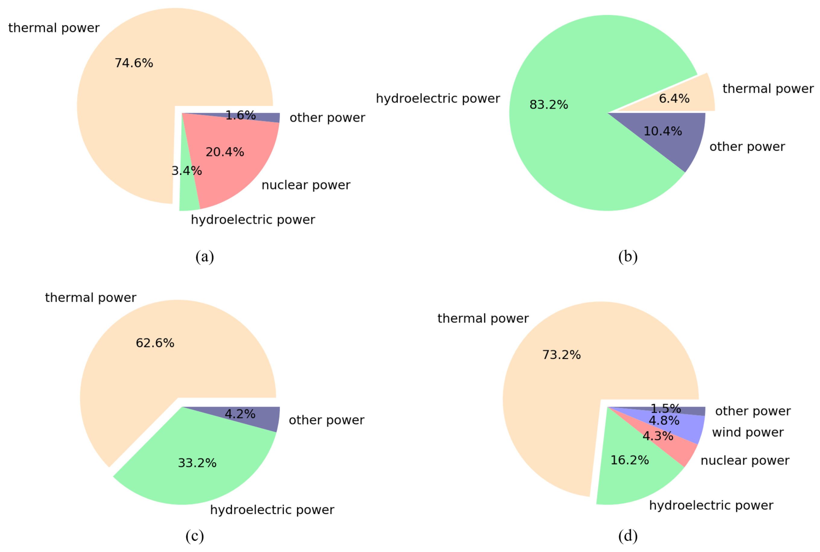
Previous research generally adopted the national power generation mix to estimate EVs CO${}_2$ emissions. A recent study [28] indicated that this will result in overestimating/underestimating the CO${}_2$ emissions by about 120% using the national power generation mix. In this paper, we updated the data of the Guangdong power generation mix from extensive reviews of research papers, yearbooks, government announcements, and so on.

To conclude, we focused on building a framework to compare the WTW CO${}_2$ emissions between battery electric buses (BEBs) and conventional diesel buses (CDBs) based on BEB sensor data in Shenzhen city. As the WTW CO${}_2$ emissions accounted for about 70–90% of the full life cycle CO${}_2$ emissions [13,14]. In addition, we obtained limited data of vehicle material for CDBs and vehicle recycling process data for both BEBS and CDBs [14].

Specifically, we reconstructed the second-by-second CDB trajectories with a modal activity-based method [27] and then estimated the CO${}_2$ emissions of CDBs with the VT-Micro model. To improve the estimation accuracy of BEB CO${}_2$ emissions, we updated the data of the Guangdong power generation mix. We compared the WTW CO${}_2$ emissions between BEBs and CDBs traveling at different speed horizons to understand the characteristics and influencing factors of CO${}_2$ emissions.

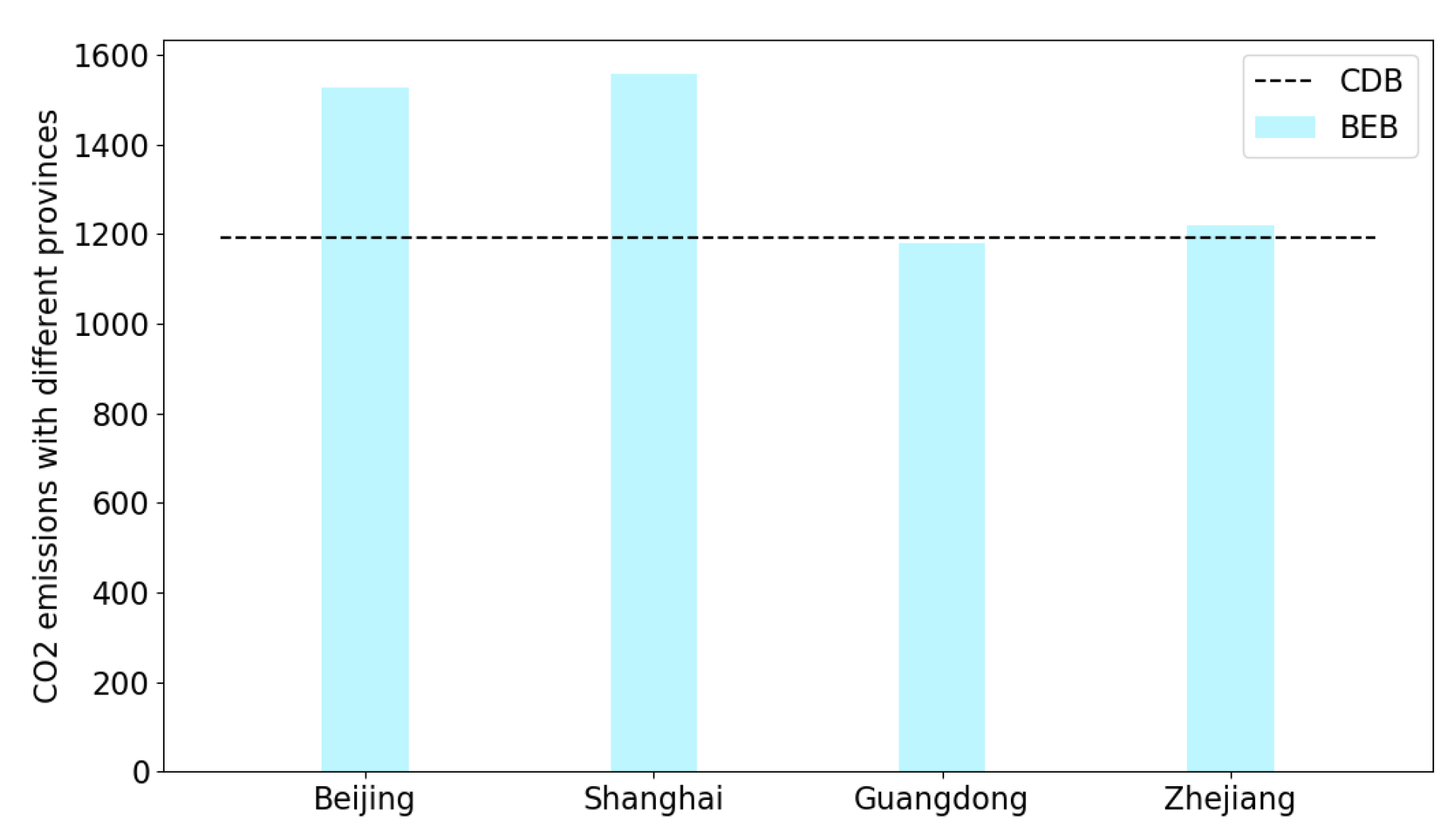
WTW CO${}_2$ emission estimation in the four provinces with the largest electric vehicle sales is presented to illustrate the importance of inter-provincial electricity transactions. We focus on the low frequency of air-conditioning usage due to the limitations of the BEB data.

The remainder of this work is organized as follows. Section 2 describes the CO${}_2$ emission estimation methods of BEBs and CDBs. In Section 3, we present the trajectory reconstruction result, and the CO${}_2$ emission comparisons between BEBs and CDBs traveling at different speed horizons. Section 4 discusses the limits of this work. Finally, we conclude the study in Section 5.

2. Methodology

2.1. Study Area and Data Description

We collected mobile sensor data from over 5000 BEBs whose sampling frequency was about 30 s. In this paper, we selected BEB data ranging from 2–8 January 2019, with more than 100 million valid records, each of which included the bus ID, log time, position information, speed, travel distance, and battery information. The battery information included the vehicle state (1: driving and 0: stall), vehicle charge state, current, voltage, SoC, and temperature.

In the data washing process, we filtered out some BEB data with abnormal traction battery data and travel mileage. For instance, it was unreasonable if the SoC of a BEB jumped over 3% in consecutive sampling intervals. Furthermore, we excluded BEBs whose travel mileage was less than 50 km/day because some running data were lost for these BEBs.

2.2. Well-to-Wheel Approach

The well-to-wheel (WTW) approach [29] has been extensively applied to evaluate the life cycle fuel consumption and environmental impact of a vehicle. The WTW approach divides the full life cycle into two processes: the fuel production process (well-to-tank, WTT) and the fuel combustion process (tank-to-well, TTW). The former process usually comprises feedstock production, transportation, fuel production, and fuel distribution. The later stage mainly represents the fuel combustion during vehicle running periods.

Referring to a previous study [9], the WTT CO${}_2$ emissions of a BEB include coal production, coal transportation, electricity production, and electricity transmission. The former two processes only contribute about 0.04% of the WTW CO${}_2$ emissions [9]. Therefore, the WTT CO${}_2$ emissions can be estimated by the greenhouse gases, regulated emissions, and energy use in the transportation (GREET) model [30] with the updated Guangdong power generation mix and electricity transmission efficiency. For the TTW process, the CO${}_2$ emissions mainly come from the charging loss of BEBs.

We determined the value of the charging loss of BEBs by referring to research papers. For CDBs, the WTT CO${}_2$ emissions come from the crude oil production and transportation, diesel production, and diesel distribution. We used the GREET model to estimate the WTT CO${}_2$ emissions. The WTT CO${}_2$ emissions contributed only 20% of the total WTW CO${}_2$ emissions; thus, we adopted the default values of the parameters in the GREET model. We applied the VT-Micro model to estimate the TTW CO${}_2$ emissions. The details of the framework for comparing CO${}_2$ emissions between BEBs and CDBs were illustrated in Figure 1.

2.3. CO${}_2$ Emission Estimation of BEBs

The use of electric vehicles provokes increased CO${}_2$ emissions from electric power generation. Due to the structures of the power grids, the CO${}_2$ emission factors vary in the different provinces in China. To estimate the WTW CO${}_2$ emissions of a BEB, it is necessary to determine the WTT CO${}_2$ emissions factor $f_{WTT}$ (kg/kWh) and electricity consumption $Q_k$.

To obtain the electricity consumption $Q_k$ during the driving process, we calculate the electricity that the BEB was charged with because the losses within the BEB system over time will not be accounted for in a precise way. During the charging process of the electric bus, the value of the state of charge (SoC) increases from a to b, and the value of the SoC decreases from b to c during the driving period. Then, we can obtain the electricity consumption of electric buses as follows:

$$Q_k=\frac{b-c}{b-a}\times {\int }_0^T{U}_k{I}_{k}dt$$

(1)

where $Q_k$ (KWh) denotes the electricity consumption, and $U_k$ (V) and $I_k$ (A) denote the charging voltage and current, respectively. The time of the charging process is T. The output voltage of the battery varies nonlinearly with the SoC value; however, the errors can be ignored for a long period.

After obtaining the electricity consumption, the CO${}_2$ emissions factor of BEB k can be calculated as:

$$e_{BEB,k}=\frac{f_{WTT}{Q}_k}{D_k}\times 100$$

(2)

where $e_{BEB,k}$ (kg/km) represents the CO${}_2$ emissions factor of BEB k, and $D_k$ (km) is the travel distance of BEB k.

For the WTT CO${}_2$ emissions factor $f_{WTT}$, we can estimate it with the well-to-wheel approach [29] by updating the data of the power structure in the GREET model [30].

2.4. CO${}_2$ Emission Estimation of CDBs

Public transport needs to arrive at the bus stops on schedule. In this sense, although BEBs and CDBs have different power systems, it can be considered that a CDB has approximate trajectories with a BEB of the same bus line. Thus, the TTW CO${}_2$ emissions of CDBs can be estimated based on the BEB trajectories.

In this paper, we estimated the WTT CO${}_2$ emissions with the default parameters in the GREET model. We applied the VT-Micro model proposed in [31] to estimate the TTW CO${}_2$ emissions of conventional buses. The required second-by-second trajectories in the VT-Micro model were estimated by the modal activity-based method [27].

The CO${}_2$ emission factor of a CDB k was estimated by Equation (3).

$$e_{CDB,k}=e_{WTT}+e_{TTW,k}=e_{WTT}+\frac{{\int }_0^T{r}_{t}dt}{1000D_k}$$

(3)

where $e_{CDB,k}$ (kg/km) denotes the CO${}_2$ emission factor of CDB k, and $e_{WTT}$ (kg/km) and $e_{TTW,k}$ (kg/km) denote the WTT and TTW CO${}_2$ emission factors, respectively. As we implemented the default values of the parameters in the GREET model, the WTT CO${}_2$ emission factors for all CDBs are the same. $r_t$ (g/s) is the instantaneous CO${}_2$ emission rate, which can be estimated by the VT-Micro model.

2.4.1. VT-Micro Model

The micro vehicle carbon dioxide emissions estimation model is characterized by Equations (4) and (5) [31]:

$$ln\left(r_t\right)=\sum _{i=0}^3\sum _{j=0}^3\left(L_{i,j}\times {\left(v_t\right)}^i\times {\left(a_t\right)}^j\right),a_t\ge 0$$

(4)

$$ln\left(r_t\right)=\sum _{i=0}^3\sum _{j=0}^3\left(M_{i,j}\times {\left(v_t\right)}^i\times {\left(a_t\right)}^j\right),a_t<0$$

(5)

where $v_t$ is the instantaneous speed of the sampling time t; $a_t$ is the instantaneous acceleration of the sampling time t; $r_t$ is the instantaneous carbon dioxide emission rate; $L_{i,j}$ and $M_{i,j}$ are the model coefficients for $r_t$ at the speed power i and acceleration power j for positive accelerations and negative accelerations, respectively.

We used the reconstructed second-by-second vehicle trajectories to estimate the variables $v_t$ and $a_t$.

2.4.2. Vehicle Trajectory Reconstruction

In this subsection, we adopt the modal-activity-based method proposed in [27] to reconstruct the vehicle trajectories. The model is comprised of two parts: the identification of the modal activity sequence and the allocation of the travel time/distance to each mode.

Modal Activity Sequence

When a public transport bus is traveling on urban roads, it experiences frequent speed reductions and stop-and-go behaviors at bus stops and traffic light intersections. The most prevalent modal activities include idling, acceleration, cruising, and deceleration.

We can extract a sequence of data pairs from a certain mobile electric bus data. The data pair includes: the start speed $v_s$, the end speed $v_e$, time interval $\Delta t$, and total travel distance $\Delta s$. A four tuple $\left[v_s,v_e,\Delta t,\Delta s\right]$ is used to denote the data pair. Given a data pair, the modal activity sequence can be identified based on the relationships among $v_s$, $v_e$ and the average speed $\overline{V}$. In this paper, we define idling, acceleration, cruising, and deceleration as $M_1$,$M_2$,$M_3$, and $M_4$, respectively. We use the vector $\mathbf{S}$ to denote the modal activity sequence. For a certain data pair $\left[v_s,v_e,\Delta t,\Delta s\right]$, the probability of different modal activity sequences is shown in

Table 1. The probabilities of different modal activity sequences.

Modal Activity Sequence	$\overline{\mathit{v}}>{\mathit{v}}_{\mathit{s}}$	$\overline{\mathit{v}}<{\mathit{v}}_{\mathit{e}}$	$\overline{\mathit{v}}<{\mathit{v}}_{\mathit{s}}$	$\overline{\mathit{v}}<{\mathit{v}}_{\mathit{s}}$	$\overline{\mathit{v}}\in \left[{\mathit{v}}_{\mathit{min}},{\mathit{v}}_{\mathit{max}}\right]$
$\mathbf{S}1=[\mathrm{M}3,\mathrm{M}2,\mathrm{M}3]$	1	0	0	1	1
$\mathbf{S}2=[\mathrm{M}3,\mathrm{M}4,\mathrm{M}3]$	0	1	1	0	1
$\mathbf{S}3=[\mathrm{M}3,\mathrm{M}2,\mathrm{M}3,\mathrm{M}1,\mathrm{M}3]$	1	1	0	0	0
$\mathbf{S}4=[\mathrm{M}3,\mathrm{M}4,\mathrm{M}3,\mathrm{M}2,\mathrm{M}3]$	0	0	1	1	0

Note: $v_{\mathit{max}}=\mathit{max}(v_s,v_e)$, $v_{\mathit{min}}=\mathit{min}(v_s,v_e)$.

.

• If the value of $\overline{V}$ is between $v_s$ and $v_e$, and $v_s<v_e$, the modal activity sequence $\mathbf{S}\mathbf{1}$ can be shown as Figure 2.
• If the value of $\overline{V}$ is between $v_s$ and $v_e$, and $v_s>v_e$, the modal activity sequence $\mathbf{S}\mathbf{2}$ can be shown as Figure 3.
• If the value of $\overline{V}>max\left(v_s,v_e\right)$, the modal activity sequence $\mathbf{S}\mathbf{3}$ can be shown as Figure 4. A bus will not change its modal activity frequently when traveling on urban roads [32]. We presume that there exists one inflection speed point $\widehat{v}$ between a data pair of $\mathbf{S}\mathbf{3}$.
• If the value of $\overline{V}<max\left(v_s,v_e\right)$), the modal activity sequence $\mathbf{S}\mathbf{4}$ can be shown as Figure 5.

According to [32], we ignored certain modal activity sequences, because these sequences occur rarely in the real world. For example, when the value of $\overline{V}$ is between $v_s$ and $v_e$, the sequences $\mathbf{S}3=[\mathrm{M}3,\mathrm{M}2,\mathrm{M}3,$ $\mathrm{M}2,\mathrm{M}3]$ and $\mathbf{S}3=[\mathrm{M}3,\mathrm{M}4,\mathrm{M}3,\mathrm{M}4,\mathrm{M}3]$ are ignored.

Given a data pair, we can identify the modal activity sequence based on the relationship among $v_s$, $v_e$, and the average speed $\overline{V}$. Another challenge was to allocate the travel time and distance for each mode of the vehicle trajectories.

Assignment of Travel Time and Distance for Each Mode

According to [27], the acceleration pace ($t/\Delta v$) followed a Gaussian distribution.

$$\zeta =\frac{t}{\Delta v}\sim N\left({\mu }_t,{\sigma }_t^2\right).$$

(6)

To simplify the model, we assumed a constant acceleration/deceleration rate during the acceleration/deceleration period. Then, we identified the value of a when the travel time of the acceleration/deceleration period was determined. For models $\mathbf{S}\mathbf{1}=[\mathrm{M}3,\mathrm{M}2,\mathrm{M}3]$ and $\mathbf{S}\mathbf{1}=[\mathrm{M}3,\mathrm{M}4,\mathrm{M}3]$, we determined the travel time and distance for each mod using Equations (7) and (8):

$$\left(v_s\times t_1\right)+\left(v_s\times t_2+0.5\times a\times t_2^2\right)+\left(v_e\times t_3\right)=\Delta s$$

(7)

$$\sum _{i=1}^3{t}_i=\Delta t$$

(8)

For the models $\mathbf{S}3=[\mathrm{M}3,\mathrm{M}2,\mathrm{M}3,\mathrm{M}1,\mathrm{M}3]$ and $\mathbf{S}4=[\mathrm{M}3,$$\mathrm{M}4,\mathrm{M}3,\mathrm{M}2,\mathrm{M}3]$, we needed to identify the inflection speed $\widehat{v}$, travel time, and distance for each mode. Referring to [27], the speed gap $\overline{v}-\widehat{v}$ (denoted as $\eta$) follows a mixed Gaussian distribution.

$$P\left(\eta \right)=\sum _{i=1}^2{w}_{i}P\left({\eta }_i|{\mu }_i,{\sigma }_i^2\right)$$

(9)

where $w_i$ is the weighting factor associated with the i-th Gaussian distribution $N\left({\mu }_i,{\sigma }_i^2\right)$ and ${\sum }_{i=1}^2{w}_i=1$.

In terms of the idling and cruising modes, we adopted the assumption in the study [27], this work assumed the travel time of the idling and cruising modes following a uniform distribution $U(0,\Delta t)$, ranging from zero to the sampling time interval. Then, we determined the travel time and distance of the other two cruising models based on the time and distance constraints ${\sum }_{i=1}^3{t}_i=\Delta t$ and ${\sum }_{i=1}^3{s}_i=\Delta s$.

2.5. Parameter Setting

To estimate the WTW CO${}_2$ emissions of BEBs and CDBs, we had to determine the parameters of the power generation mix in Guangdong, the electricity transmission efficiency, and the charging efficiency. We needed to identify the parameters in the VT-Micro model and the modal-activity-based model.

2.5.1. Parameter Setting of Electricity Mix

The Guangdong province generated 469.4 billion kwh of power and purchased 193.0 billion kwh of power in 2018 [9]. Specifically, the West–East electricity transmission project transmitted approximately 169.8 billion of power to Guangdong. Among them, Yunnan and Guizhou province transmitted about 133.6 billion kwh and 36.2 billion kwh of power to Guangdong [9], and the remaining 23.2 billion kwh of power were purchased from the State Grid of China [9]. Figure 6 presents the detailed electricity mix [33] of Guangdong, Yunnan, Guizhou, and the State Grid of China in 2018. The transmission efficiency of electricity was 93.3% according to a recent study [9]. The charging efficiency of BEBs was estimated to be 69% [14]. We used the default values in the GREET model to determine the other parameters.

2.5.2. Parameter Settings of the VT-Micro Model

The developer of the VT-Micro model provided software to estimate the coefficient $L_{i,j}$ and $M_{i,j}$ for CO${}_2$ emission [34], the results are presented in

Table 2. Coefficient $L_{i,j}$ for the CO${}_2$ emissions of the VT-Micro model.

	$\mathit{j}=0$	$\mathit{j}=1$	$\mathit{j}=2$	$\mathit{j}=3$
$i=0$	6.916	0.217	$2.354\times {10}^{-4}$	$-3.639\times {10}^{-4}$
$i=1$	−0.02754	$-0.968\times {10}^{-2}$	$-0.175\times {10}^{-2}$	$8.35\times {10}^{-5}$
$i=2$	$-2.070\times {10}^{-4}$	$-1.0138\times {10}^{-4}$	$1.966\times {10}^{-5}$	$-1.02\times {10}^{-6}$
$i=3$	$9.80\times {10}^{-7}$	$3.66\times {10}^{-7}$	$-1.08\times {10}^{-7}$	$8.50\times {10}^{-9}$

and

Table 3. Coefficient $M_{i,j}$ for the CO${}_2$ emissions of the VT-Micro model.

	$\mathit{j}=0$	$\mathit{j}=1$	$\mathit{j}=2$	$\mathit{j}=3$
$i=0$	6.915	−0.032	$9.17\times {10}^{-3}$	$-2.88\times {10}^{-4}$
$i=1$	0.0284	$8.53\times {10}^{-3}$	$1.15\times {10}^{-3}$	$-3.06\times {10}^{-6}$
$i=2$	$-2.26\times {10}^{-4}$	$-6.594\times {10}^{-5}$	$-1.289\times {10}^{-5}$	$-2.68\times {10}^{-7}$
$i=3$	$1.11\times {10}^{-6}$	$3.20\times {10}^{-7}$	$7.56\times {10}^{-8}$	$2.95\times {10}^{-9}$

.

2.5.3. Parameter Settings of the Modal-Activity-Based Model

A recent study [32] applied the maximum likelihood estimation method to estimate the ${\mu }_t$ and ${\sigma }_t^2$ of the Gaussian distribution $\zeta \sim N\left({\mu }_t,{\sigma }_t^2\right)$.

Table 4. The calibrated parameters of the acceleration/deceleration process.

Mode	Variable	${\mathit{\mu }}_{\mathit{t}}$	${\mathit{\sigma }}_{\mathit{t}}^2$
Acceleration	$\zeta$	0.814	0.311
Deceleration	$\zeta$	1.099	0.582

presents the calibrated parameters of the acceleration/deceleration process. We adopted the EM algorithm to learn the parameters $\eta$ of the Gaussian Mixture Model (GMM) based on the NGSIM U.S. 101 dataset.

Table 5. Parameters of GMM models on the arterial road.

Variable	${\mathit{w}}_{\mathit{i}}$	${\mathit{\mu }}_{\mathit{i}}$	${\mathit{\sigma }}_{\mathit{i}}^2$
${\eta }_1$	0.471	−4.439	5.482
${\eta }_2$	0.529	5.418	3.249

shows the parameters of the GMM models on the arterial road.

3. Experiments Results

3.1. Trajectory Reconstruction

We applied the modal activity-based method to reconstruct the second-by-second trajectories from low-resolution mobile sensor data.

Figure 7 presents the reconstruction trajectories results of all sampling electric buses. As a result, the modal activity-based method can reconstruct the second-by-second trajectories for all sampling BEBs with small estimated errors. Particularly, we show the results for a particular electric bus whose ID was “LC06S24K7G1004875” in Figure 7. The specific electric bus data was collected from 4 January 2019, with a travel distance of 91.399 km. The distance error between the estimated trajectory and true trajectory was 2.271 km. The trajectory reconstructed by the modal-activity-based vehicle estimation method was approximate to the actual trajectory. The results demonstrate the good performance of the modal-activity-based vehicle estimation method for trajectory reconstruction.

Table 6. Probability of different modal activity sequence.

${\mathit{L}}_{\mathit{total}}$ (km)	${\mathit{L}}_{\mathit{aver}}$ (km)	${\mathit{ϵ}}_{\mathit{min}}$ (km)	${\mathit{ϵ}}_{\mathit{max}}$ (km)	${\mathit{ϵ}}_{\mathit{aver}}$ (km)
774,782.100	192.924	0.016	9.123	4.649

Note: $L_{\mathit{total}}$ and $L_{\mathit{aver}}$ are the total travel distance and the average travel distance; ${ϵ}_{\mathit{min}}$, ${ϵ}_{\mathit{max}}$, ${ϵ}_{\mathit{aver}}$ are the minimal, maximum, and average estimated distance error, respectively.

showed the trajectory reconstruction results for sampling BEBs. The table revealed that the average estimated distance error and the maximum estimated distance error were 4.649 and 9.123 km, respectively. The reasons are from the following two aspects:

• In the modal activity-based vehicle trajectory estimation method, we assumed three distributions to reconstruct the trajectory, the parameters were calibrated from NGSIM U.S. 101 dataset. The values of these parameters may be different for our mobile electric bus data.
• In the acceleration and deceleration periods, we presumed the value of acceleration/deceleration rate was constant. As we aimed to compare the CO${}_2$ emissions of electric buses and conventional buses in large-scale areas, the distance errors of the modal-activity-based estimation method are acceptable.

3.2. Impacts of Speed on CO${}_2$ Emissions

As we estimated the CO${}_2$ emissions of CDBs with a microscopic model, we can evaluate the CO${}_2$ emission between BEBs and CDBs under different horizons of speed. The average speed of the sampled buses ranged from 7 to 20 km/h. Referring to [13], we divided the three-speed horizons as <10, 10–15, and 15–20 km/h.

Figure 8 illustrates the WTW CO${}_2$ emissions between BEBs and CDBs on different speed horizons. The WTW CO${}_2$ emissions factors on three speed horizons for BEBs were 1.023, 0.943, and 0.918 kg/km, respectively. While the CO${}_2$ emissions factors for CDBs were 1.341, 1.192, and 1.109 kg/km on these speed horizons. As a result, a BEB reduced CO${}_2$ emissions by 17.2–23.7% compared with a CDB. The CO${}_2$ reduction benefits were similar to those shown in prior research [13,14], which reported that BEBs can reduce CO${}_2$ emissions by 19–35%.

The WTW CO${}_2$ emission factors for BEBs ranged from 0.9 to 1.014 kg/km, and this value was slightly lower than those shown in prior works [13,14], which showed that the tested BEBs emitted 1.1 kg CO${}_2$/km on average. The average speed of the sampled BEBs was 17.6 km/h, while the BEBs tested in prior studies [13,14] ran at a speed of 15 km/h. The thermal power occupied a lower proportion in the power generation mix in our study compared with that in the previous studies [13,14]. Hence, the estimated CO${}_2$ emission factor of BEBs was reasonable.

BEBs reduced more CO${}_2$ emissions in comparison with CDB when the transit bus operated at a low speed. The reason was that, when the bus traveled in rush-hour traffic, it experienced frequent stop-and-go behaviors, and the brake energy cycling system of BEB can restore energy to the battery package. When the average speed increased, such benefits against CDB became less important.

The default WTT CO${}_2$ emissions factor for CDBs was 0.32 kg/km, and the TTW CO${}_2$ emissions contributed more than 73.1% of the WTW CO${}_2$ emissions. Specifically, CDBs emitted CO${}_2$ with 1.009–1.341 kg/km, while the average WTW CO${}_2$ emissions factor for the tested CDBs in 2014 was 1.4 kg/km [13,14]. The estimation result was acceptable because various technologies have been developed to reduce CO${}_2$ emissions for CDBs in recent years.

As diesel buses still occupy the largest market share in China’s bus market, the government and private enterprises need to continuously improve the diesel-driven system to reduce the real-world CO${}_2$ emissions of diesel. The reduction rate of BEB on WTW CO${}_2$ emissions was nonlinear and could achieve a more marginal CO${}_2$ reduction under a lower average speed. Such a phenomenon was more obvious with CDB. This circumstance implies that BEBs were supposed to have obvious CO${}_2$ emission reductions over CDBs, because public transit buses travel at low speeds on urban roads.

The average speed plays an important part in WTW CO${}_2$ emissions, especially for public transit buses. As they need to arrive at the bus stops on schedule, the ratio of buses traveling at low speeds is commonly high. Figure 9 presents the ratio of driving speed for three different speed horizons of buses in real operational scenarios. The ratio represents the proportion of travel time at this speed to the total travel time of the vehicle.

The light blue bar denotes the average value of the ratio, while the length of the orange line denotes the standard value of the ratio. A bus with higher average speed owned a larger proportion of the travel time operated at high speed. Specifically, a bus with an average of 15–20 km/h traveled half of the time with a speed over 20 km/h.

Three different speed horizons buses had similar ratios of travel time operated at speeds of 10–15 and 15–20 km/h, and the values of these two ratios were stable for all buses. The average speed of bus travel slower than 15 km/h accounted for about 97% of the sampled buses, and the bus traveled at a speed lower than 10 km/h nearly half of the time. In this sense, it is critical for the traffic manager to improve the efficiency of the road networks. For example, the green wave control on arterial roads.

3.3. CO${}_2$ Emissions Comparisons in Different Regions

Intuitively, the reduction rates of CO${}_2$ emissions vary with the CO${}_2$ emission intensities of the power grid. Existing studies demonstrated that the power structures have great impacts on the CO${}_2$ emission reduction benefits of electric vehicles [35]. Therefore, it is crucial to evaluate the WTW CO${}_2$ emissions in different regions in China.

Base on the China National Bureau of Statistics data [33], we evaluated CO${}_2$ emissions in the four provinces with the largest electric vehicle sales, the thermal power share and total electricity generation of these four provinces are presented in

Table 7. The power generation mix in the four provinces with the largest electric vehicle sales in China.

Province	Beijing	Shanghai	Guangdong	Zhejiang
Thermal power (billion kwh)	422.8	813.7	3260.1	2583.4
Total (billion kwh)	437	824.7	4369.6	3352.8
Thermal power share	96.7%	98.6%	74.6%	77.1%

. In the GREET model, the CO${}_2$ emissions of electricity generation had an approximately linear relationship with the thermal power share. Without considering the inter-provincial electricity transactions, we can easily calculate the CO${}_2$ emissions for four provinces given the electricity transmission efficiency and charging efficiency of BEBs.

Due to the lack of operation data of transit buses in other provinces, we assumed the transit buses in other provinces had similar operation data. The CO${}_2$ emissions of BEBs in different cities are shown in Figure 10. Without considering the inter-provincial electricity transactions, the BEB could achieve a CO${}_2$ emission reduction benefit only in Guangdong. The above section indicated that a BEB could achieve about 18.0–23.9% CO${}_2$ emission reduction benefits compared with a CDB.

In practice, the BEBs had better real-world CO${}_2$ emissions performances in Beijing, Shanghai, and Zhejiang similarly, since a major part of their electricity consumption was transmitted from other provinces with high hydropower shares. Therefore, it is critical for the provincial government to pay more attention to inter-provincial electricity transactions. The inter-provincial electricity transactions are efficient measures to improve the energy structure of the power mix, so that more CO${}_2$ reduction benefits can be achieved by BEB adoption.

4. Discussion

The CO${}_2$ emissions of a public transit bus are dependent on the ambient temperature. Prior studies [13,14] claimed that the CO${}_2$ emissions of CDBs and BEBs with air-conditioning use increased 48% and 23% compared to the operation conditions without air-conditioning use. At this time, we could only obtain the BEB data in January for Shenzhen; we will investigate the CO${}_2$ emissions across different seasons after we obtain the BEB data of a whole year.

Fortunately, a study [13] demonstrated that BEB provides significant CO${}_2$ emission reduction benefits compared with CDB when operating in hot weather with air-conditioning use. Therefore, we conclude that the CO${}_2$ emission reduction benefit estimation was reasonable and even slightly conservative in our paper due to the frequency of air-conditioning usage being the lowest in January in Shenzhen.

Due to the unavailability of the city-scale CDBs data in Shenzhen, we utilized the BEB trajectories to estimate the WTW CO${}_2$ emissions for CDBs. A previous study [36] indicated that BEBs are driven more aggressively than CDBs. Fortunately, the experimental results indicated that the estimated errors were acceptable. The CDBs emitted CO${}_2$ with 1.009–1.341 kg/km in our paper, while the average WTW CO${}_2$ emissions factor for the tested CDBs in previous studies [13,14] was 1.4 kg/km. Considering that various technologies have been developed to reduce CO${}_2$ emissions for CDBs in recent years, the estimated CO${}_2$ emission factor for CDBs is acceptable. The experiments showed that BEBs could reduce CO${}_2$ emissions by 18.0–23.9% compared with CDBs. The CO${}_2$ reduction benefits are similar to those shown in prior research [13,14], which reported that BEBs could reduce CO${}_2$ emissions by 19–35%.

Some factors that may influence the CO${}_2$ emissions for CDBs are ignored in Equations (4) and (5), such as auxiliary power (power steering, air compressor, and so on), which is independent of the trajectory. However, auxiliary power is included in the calculation of the BEB power consumption in Equation (1). Though the experimental results validated the effectiveness of our proposed method, we hope to design a more delicate model that can consider more factors to estimate CO${}_2$ emissions in future work.

We aimed to compare CO${}_2$ emissions between BEBs and CDBs in this paper. To further validate the advantage of BEB adoption, more greenhouse gases are required to compare between BEBs and CDBs, and we plan to utilize CO${}_2$ emissions to evaluate multiple greenhouse gas emissions between BEBs and CDBs in our future work.

5. Conclusions

The electrification of public transit buses plays an important role in reducing CO${}_2$ emissions. To evaluate the CO${}_2$ emission effects with the adoption of BEBs at the city level, we compared the CO${}_2$ emissions between BEBs and CDBs based on the low sampling frequency BEB data in Shenzhen city for the low frequency of air-conditioning usage conditions. We applied the VT-Micro model to estimate the real-world CO${}_2$ emissions of CDBs, and a modal activity-based method was used to reconstruct the second-by-second transit bus trajectories as the input of the VT-Micro model. We updated the data of the Guangdong power generation mix from an extensive review of papers. We draw the following conclusions from this paper:

• A BEB achieved approximately an 18.0–23.9% CO${}_2$ emission reduction benefit in comparison with a CDB when the frequency of air-conditioning usage was low.
• A BEB tended to reduce more CO${}_2$ emissions compared with a CDB when the transit bus traveled at a low speed.
• During the operation process of BEB, nearly half of the time, the bus traveled at a speed lower than 10 km/h.
• The inter-provincial electricity transactions were efficient measures to promote the adoption of BEBs, as they helped to improve the energy structure of the electricity mix.

The above observations can help to plan and dispatch public transport vehicles based on the CO${}_2$ emission intensity in different cities. However, there are still some limitations to this work. We only considered transit buses in this paper, the CO${}_2$ emission impacts of substituting electric vehicles for light-duty vehicles must be studied with more data. In future work, we will explore the life cycle CO${}_2$ emissions between electric buses and conventional buses.