Abstract
The main purpose of this research is to study the predictive power of behavioural life profile models for mortgages using machine learning techniques and emerging languages from the same data sets. Based on the results, banks can determine whether the predictive power of the model can be improved regarding estimates of probability of redemption, and probability of internal transfer beyond traditional techniques. Model training will take place using algorithms based on machine learning such as: random forests, extreme gradient, boosting, light gradient boosting, Adaboost, and ExtraTrees. To perform simulations on fast learning and permit testing of hypotheses, the IBM cloud environment and the Watson proven analytical environment will be used, in order to maximize the value derived from the investment and determine the decision on the implementation and modelling strategy for business disciplines. Therefore, these factors could provide a solid basis for the sustainable development of the mortgage market, and the approach in this research is a starting point for identifying the best decisions taken by banking institutions to contribute to the sustainable development of mortgage lending.
1. Introduction
In general, the concept of sustainable development encompasses economic, social, and environmental considerations that can evolve in interdependence, supporting each other. Romania’s national economy can be seen as a complex, adaptive cybernetic system, because several properties of this system can be identified, such as connectivity, interdependence, emergence, coevolution, feedback, etc.
Romania’s specific development needs and ensuring policy compatibility between economic, social and environmental issues with the main strand of development within the EU requires active and responsible involvement of central and local public institutions, of the private sector, professional associations, social partners and civil society in maintaining a business environment favourable to domestic and foreign capital investments intended for the modernization and sustainable development of the country.
According to the National Strategy for the Sustainable Development of Romania Horizons 2013–2020–2030, developed by the Romanian Government in collaboration with the Ministry of Environment and Sustainable Development [1,2], supporting the development of the real estate market and mortgage credit is a sustainable development strategy in Romania, so the bank plays an important role in the process of granting mortgages to support the sustainable development strategy. The way in which the bank ensures the mortgage lending process directly influences the proposed strategy because the application of an efficient credit risk management on the mortgage lending process impacts the demand and supply on the market.
Thus, this paper analyses mortgage behavioural life profile models, using machine learning techniques in order to identify whether machine learning techniques can contribute to better models than traditional techniques, so as to maintain a balance between the demand and supply of mortgages. This balance ensures both stability in the national economic environment and contributes to the sustainable development of the country.
Artificial intelligence, or AI, is human information exposed by machines. Artificial intelligence has an impact on the cognitive abilities of a machine. Early AI systems used model matching systems and expert systems.
Artificial intelligence (AI) or machine intelligence (MI) is a field of study that aims to provide cognitive powers to computers to program them to learn and solve various problems.
Machine learning (ML) is a branch of AI, an approach to achieving artificial intelligence, which helps computer programs, based on input data, to get out of the system, thus provided that they have the ability to solve data-based problems.
The idea behind machine learning (ML) is that the machine can learn without human intervention, it must find a way to learn how to solve a task, knowing the input data.
The role of banking institutions is very important because they have the role of mobilizing the financial resources of the actors of an economic market (individuals or legal entities) and directing them towards viable, economic areas for the sustainable development of their systems and their support. A bank is an economic agent that grants loans and receives in deposit money deposits from other economic agents and from the population. Such a definition is necessary in order to be able to distinguish the bank from other financial intermediaries, because the prudential rules in the case of banks are much stricter. The definition insists on the traditional central activities within the commercial banks and in our research, we will insist on the activity of granting loans.
In an economy in which there are more and more episodes of turbulence or even chaos, commercial banks must be pillars of stability and restore macroeconomic balance. However, the purposes of commercial banks are only indirectly related to such objectives because they, like any market economy system, act in order to make a profit, and their operation must be seen especially from this perspective.
In studying and analysing any behaviour of a national or global economic system, the bank may be the most sensitive institution with a significant impact on the entire system. The 2007–2009 financial crisis is an eloquent example of how the interconnection between financial institutions can pose a systemic risk to the entire financial system with an impact on the global economy. When a highly interconnected institution is affected by a negative impact event, such as Lehman Brothers, its counterparties may also experience losses and limited access to liquidity [3].
The effects of the crisis have been felt globally. At the level of the Romanian economy, the event generated a chaotic policy of human resources management, the excessive increase of income taxes, the government’s hesitation regarding the oversized public sector. These were just a few of the effects of the crisis [4].
The main traditional activity of banking institutions is lending. At the same time, credit management and the correct management of risks in this field are another challenge for great specialists. Banking is becoming more and more complex, and that should make us think: do we know everything we need to know about banks and their business? Is it enough to be guided by the bank’s staff to make a decision? Could knowing the mechanism of the functioning of this institution provide us with more than just useless information? Do we have enough methods to prevent potential systemic shocks with contagion that can cause economic crises [5]?
Lending institutions offer a wide range of such products as unsecured personal loans, credit card, overdraft and mortgages. The latter category is an important class in any bank’s portfolio because large volumes are granted in the long run and economic, political, social, and environmental events are just a few factors that can disrupt the stability of the banking system and the life cycle of the mortgage.
In a modern economy, the financial sector plays an important role due to the financial intermediation, respectively the channelling of funds from depositors to investors, which it provides.
A solid and efficient financial sector encourages the accumulation of savings and allows their allocation to the most productive investments, thus supporting through innovation the economic growth. In Europe, the main financial intermediaries are banks. Bank loans are also used to finance the needs of households, in particular to alleviate the vulnerability over time of their customers’ consumption pattern and help them invest in real estate [6].
An excessive increase in loans for home purchase could cause speculative price bubbles in the real estate market. The subsequent explosion of such a bubble can be very destabilizing for the financial sector and for the economy as a whole [7].
The rest of this paper is organized as follows. In Section 2, we review the preceding literature on the machine learning techniques used in developing the life cycle of the mortgage. Section 3 explains the loans portfolio in Romanian banking institutions and some mortgage loan characteristics. Moreover, we describe the banking subsystem of credit management as cybernetics systems. Section 4 describes the machine learning techniques which we used in the case study. In Section 5, we validated each machine learning technique to see which of them offers the best results in terms of the model accuracy and performance. Finally, we offer conclusions and implications.
2. The Stage of the Knowledge in the Field
2.1. Literature Review
In Romania, there is no research to compare the evaluation of models based on machine learning with traditional models. In the context of sustainable development, this paper is a starting point for boosting banks in the use of machine learning techniques, but also the promotion of digitization. Digitization has become a necessity to keep up with evolution, it has expanded to the global economy, which makes the “digital” artefact change the environment in which we work, trade, collaborate, and control the workforce, institutions and markets throughout the world. Gradually, digitization methods will develop as they evolve and change, accompanied by an understanding of the societal implications of change generated by the growth of the digital phenomenon and the cyberization of the economy. Various studies show the competitive results of machine learning techniques when compared with logistic regression, which is traditionally used in credit scoring classification analysis.
Maisa Cardoso Aniceto, Flavio Barboza, and Herbert Kimura in the article “Machine learning predictivity applied to consumer creditworthiness” state that credit risk assessment has a significant role for banking institutions, especially default prediction is one of the most challenging activities of banking specialists for efficient credit risk management. The authors analyse in their study the appropriate use of loan classification models using machine learning techniques. They use support vector machine, decision trees, AdaBoost, and random forest models to compare their predictive accuracy with traditional models based on logistic regression. The authors concluded that the best method, given the performance of AUC-based metrics, was this AdaBoost technique, followed by random forest [8].
Another paper that compares the predictive power of credit scoring models based on machine learning techniques with traditional models is “How do machine learning and non-traditional data affect credit scoring? New evidence from a Chinese fintech firm”, elaborated by Leonardo Gambacorta, Yiping Huang, Han Qiu, and Jingyi Wang. The authors perform the analysis on a top fintech company in China for a period of five months in 2017 in which they test the performance of various default and loss prediction models. The analysis performed both in normal periods and when the economy is subject to shock, such as regulatory changes in China’s shadow banking policy that have led to declining lending and deteriorating lending conditions. They found that, when using machine learning techniques, the power of prediction is much better than in traditional cases because they are better able to predict losses and default in the presence of a shock that can unbalance the banking system and even the country’s economy [9].
Aseem Mital and Dr. Atul Varshneya [10] are of the opinion that it is obvious that artificial intelligence and machine learning constitute the future of consumer loans. They believe that machine learning is an efficient and effective solution as credit processing and monitoring of fintech activities are undertaken by machines.
Santiago Carbo-Valverde, Pedro Cuadros-Solas, Francisco Rodríguez-Fernández present another very important aspect: the concept of bank digitization. They analyse in their research how machine learning techniques help to design effective strategies that allow the rapid transition to the digital context [11].
Peter Martey Addo, Dominique Guegan, and Bertrand Hassani analysed in their paper [12] that due to advanced technology in the context of an era of large data volumes, banks need to adapt and redevelop their business models. A key element, in their opinion, is the activity of credit risk prediction, together with the efficient monitoring and processing of loans. They use ML techniques to predict the probability of defaulting on the loan. The conclusion of the research was that tree-based models are much more stable than models based on multilayer artificial neural networks and that this requires more analysis and the answer to more questions related to the intensive use of deep learning systems.
In “Deep Learning for Mortgage Risk” [13], the authors develop a deep-learning model of mortgage risk to analyse the performance of more than 120 million mortgages in the United States. The authors believe that the findings made by them in the research have important implications for the mortgage guarantee security investors, rating agencies and homeowners.
An interesting analysis is made by Yang Yu et al. [14] which shows the usefulness of machine learning techniques in a less researched field. This also supports the main idea of this article, that any economic unit, whether we are talking about the company or the bank must use machine learning techniques and artificial intelligence to adapt to the environment and to perform.
The literature shows the use of ML techniques to improve the accuracy of prediction of mortgage models. Most of them chose 3–4 ML techniques to conduct the research. Taking into account the research gap in Romania related to the subject of the paper, we will test eight ML techniques to reconstruct the life profile model of mortgage behaviour in order to show that the results in terms of accuracy are much better.
2.2. Overview of the Proposed Techniques
In recent years, machine learning (ML) and, in particular, its deep learning (DL) subcomponent, have made impressive progress. The techniques developed in these two fields are now able to analyse and learn from huge amounts of real-world examples in a different format. Although the number of machine learning algorithms is expanding and growing, their implementations through frameworks and libraries are also expanding and growing. Software development in this area is rapid with a large number of open-source software from academia, industry, start-ups or wider open-source communities [15].
Data mining (DM) is the main stage in the process of discovering knowledge that seeks to extract interesting and potentially useful information from data. Although during this work, the term “data mining” is primarily aimed at large-scale data mining, many techniques that work well for large-scale data sets can also be effectively applied to large-scale data mining. smaller data. Data mining can serve as a foundation for artificial intelligence and machine learning. Many techniques in this direction can be grouped in one of the following fields [16]:
AI is any technique that aims to allow computers to mimic human behaviour, including machine learning, natural language processing (NLP), language synthesis, computer vision, robotics, sensor analysis, optimization, and simulation.
Machine learning (ML) is a subset of AI techniques that allows computer systems to learn from previous experience (i.e., data observations) and improve their behaviour for a particular task. ML techniques include support vector machines (SVM), decision trees, Bayes learning, k-means clustering, association rules, regression, neural networks, and more.
Neural networks or artificial NNs are a subset of ML techniques, which are inspired by the biological neuron. These are usually described as a lot of interconnected units, called artificial neurons, organized in layers [15,17].
According to Yang Yu et al., they conducted a research that has as main objective the investigation of how different computational tools are used compared to the models proposed by ML and the traditional, empirical ones. They believe that, compared to empirical models, ML methods have superior advantages in modelling the complexity of a subject in attention because they take into account several variables and their behaviour in the model, always testing the accuracy of model evaluation between the current situation and the predicted situation.
The topicality of this article is that in Romania the realisation and testing of credit models is based on the traditional approach. Considering the fact that we meet everywhere Artificial Intelligence, living in an era of large volume of data and information, AI transforming business analysis, the health sector or banking sector. Compared to traditional methods, machine learning involves learning algorithms based on previous experiences. Due to these situations, the implications of economic cybernetics and machine learning must develop exponentially in order to keep pace with evolution and adaptation to the current economic context. Another aspect that we approach in this paper is used to adjust the hyper parameters in machine learning algorithms in order to build models as efficiently as possible.
3. Loan Portfolio in Romanian Banking Institutions
The bank is seen as an eloquent example of a complex adaptive system because all the properties of this system are found, some in a more blurred form, others more obvious. Connectivity and interdependence with other systems in the economy are supported by the fact that commercial banks would have no economic reason if they were not connected through cash flows, but also information, with other types of economic systems, such as companies or other banks. The commercial banking system co-evolves in the economic environment with the other complex adaptive systems, this coevolution being characterized by the existence of a fitness landscape that each bank goes through, a landscape that changes under the influence of laws and regulations on banks, but also under the influence of economic performance, environmental agents [18].
One of the important subsystems of a bank is that of credit management, being also one of the activities on which the bank relies to generate profit. Between the credit management subsystem and the credit market, feedback loops are created which are formed as follows: on the credit market there are credit requests sent to the credit management subsystem, and this provides the required credits. On the other hand, the interest paid or the amounts repaid are returned to the bank from the credit market. It is obvious that there is a direct, strong link between the volume of loans granted and the interest rate, because the higher the volume of loans, the higher the interest paid. The structure of the loan portfolios offered by the Commercial Banks in Romania is given in Figure 1. The largest loan volumes are generated by secured loans. This article focuses on Mortgage Credit.
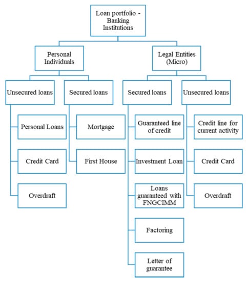
Figure 1.
Loan portfolio—Romanian Banking Institution. Source: The design is done by the authors.
3.1. Mortgage Loan Characteristics
The prepayment and credit performance of each mortgage-backed securities (MBS) are collectively determined by the features presented below. The characteristics of a loan can collectively determine both its performance and the way in which the advance payment can be made. The following table (Table 1) describes the most important features of a mortgage loan.

Table 1.
The most important characteristics of a mortgage loan.
In Romania, the minimum amount contracted for a mortgage loan is 45,000 Ron and the maximum amount you can obtain is up to 85% of the value of the investment, for a maximum term of 30 years. The loan limit is established depending on the income that a debtor has at the time he applies for the loan and the existing degree of indebtedness. In the last decade, credit scores are being used more and more by the financial industry. This has become an important factor that is analysed as part of mortgage assessments. The credit score is a quantitative measure of probability derived empirically that a borrower will repay a debt. Credit scores are generated from models that have been developed from statistical studies of historical data and used as input from the borrower’s credit history. FICO scores are tabulated by an independent credit bureau, using a model created by Fair Isaac Corporation (FICO). These scores range from 350 to 900, with higher values scores that indicate a lower risk [15].
Loan to value (LTV) represents the level of advance that a debtor needs to access the requested loan, i.e., it represents the percentage of the value of the property that is borrowed as a mortgage. The most important factor that determines the performance of a loan is the combined loan to value (CLTV) ratio, according to Laurie S. Goodman et al. [13]. When a customer already has a mortgage on a property and requested another property, the CLTV ratio is used. This represents the sum between the first mortgage elements and the second one divided at the housing level.
The DTI (debt to income) ratio is an indicator used by the bank in the lending process to analyse what is reported between the client’s income before eliminating income taxes and other deductions compared to the debts he has. More specifically, it is the percentage of a customer’s gross monthly income that is taken into account for the payment of the debts of a loan [17]. In the lending process, banks analyse several variables that make up the scorecard model. The classification of companies (client’s employer) enters the structure of the scorecard model and the variable type of company classifies companies according to private capital, foreign or public institutions. Depending on the national or international regulations to which the banks are subject, they have a maximum degree of exposure per customer for each type of loan granted from the bank’s portfolio. This is measured by the exposure indicator [18,19].
Another important aspect that the bank analyses in the pre-lending stage is the correct identification of the credit client’s need (loan purpose). Thus, depending on this need, several types of loans can be recommended, such as: mortgage, real estate, Prima Casa (First House), personal loans, credit card or overdraft. Depending on the loan requested by the client, an interest rate is established which is composed of a fixed margin regulated by the National Bank of Romania (for Romanian banks) and the variable or fixed margin of the creditor bank. The whole lending process is followed by a complex set of documentation consisting of documents issued by the bank such as credit agreement, credit application form or credit application, or other documents provided by the client at the request of the bank, depending on the purpose of the loan, such as income supporting documents, cadastral documentation, sale-purchase contract, etc. Depending on the correctness and completeness of the documentation (full documentation), the credit can be granted or not [20,21].
3.2. The Cybernetics Banking Subsystem of Credit Management
Cybernetics is the science of communication and control that studies the adaptation of complex systems to complex environments (systems). The object of study of current cybernetics is the complex adaptive system. In its evolution as a science, cybernetics has undergone transformations that have led to the need to talk about first-order cybernetics, then about second-order cybernetics and, after 2000, about third-order cybernetics [22,23].
Cybernetics as an interdisciplinary science was formed before the 1948s when several prominent personalities in the forerunners of cybernetics approached this concept in various fields. Here, we mention some notable personalities such as Réné Descartes, Henry Poincare, Stefan Odobleja, and Andre Marie Ampere. The founders of cybernetics are considered Norbert Wiener, Warren McCulloch & Walter Pitts, and Gregory Bateson when they highlighted cybernetics as the science of communication and control in 1948. Later, Ross Ashby, John von Neumann, Stafford Beer, Ilya Prigogine, and other prominent personalities highlighted the importance of fundamental understanding of the science of cybernetics, personalities considered pioneers of cybernetics. Currently, we are studying third order cybernetics and the sciences of complexity and here we mention some important personalities such as Stuart Kauffman, Stephan Wolfram, and Stuart Umpleby [22,23,24].
The object of study of current cybernetics is the complex adaptive system. Complex adaptive systems are made up of many independent agents competing on resources, where all agents have different strategies, adaptability and are naturally subject to selective pressures. These systems are evolutionary, self-organized, and decentralized. The fiercer the competition, the higher the rate of experimentation, birth, and death, and the higher the capacity for mutation and adaptation of individual agents, the greater the resistance, anti-fragility, and impact of the overall system. What works well spreads, what doesn’t work well dissolves [25,26].
Complex adaptive systems are found all around us, and the science of complexity confirms that the vast majority of real systems are complex. Natural ecosystems, e.g., the atmospheric system, road traffic, social organizations, terrorist groups, markets, etc. are complex adaptive systems.
The economy, seen as a complex adaptive system, has a structure consisting of a multitude of distinct cybernetics systems, ranging from enterprise to the global economy system. The bank is an example of a complex adaptive system. A bank is an economic agent that grants loans and receives in deposit money deposits from other economic agents and from the population. The existence of commercial banks is justified by the role they play in the process of allocating resources, more precisely in the allocation of capital. Analysing the bank as a complex adaptive system, it can be seen that all the properties of these systems are found, some in more obvious forms, others more blurred. This shows us that important economic systems, regardless of their nature and functions, fall into the category of complex adaptive systems, the economy itself as a whole representing such a system [27].
In general, the subsystems of a commercial bank can be classified into five components (according to Figure 2): credit management, deposits, risks, the funds insurance subsystem and the treasury subsystem. One of the most important cyber subsystems of the commercial bank is the credit management subsystem. In essence, the credit management subsystem represents the interface between the commercial bank and the credit market. It receives credit applications from companies and households, analyses them and, in accordance with the bank’s rules, approves them. Through this subsystem, the approved credits are sent to companies and households, following, afterwards, the collection of interests and rates related to the granted credits. This subsystem continuously sends to the risk management subsystem information on credit applications and receives from its information on credit risk. Moreover, the requests regarding the monetary funds necessary to cover the granted credits are sent to the subsystem of the bank’s treasury, which, following these requests, provides the necessary funds for granting the credits.
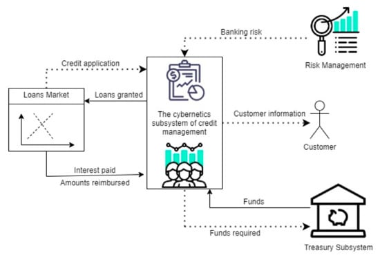
Figure 2.
Cybernetics subsystem of credit management. Source: The design is done by the authors in draw.io.
It is observed at the level of this subsystem the formation of a double feedback loop between it and the credit market. Thus, credit applications are followed by the granting of loans, obviously at a lower volume than the applications addressed to the bank, with some of the applications being rejected due to the banking risks involved.
4. Materials and Methods
An important part of machine learning is given by the concept of classification because it offers a complex view of the groups of classes that belong to certain observations. The ability to accurately classify certain observations is a valuable analysis for many business applications, not just for banks. Logistic regression, the naive Bayesian classifier, or decision trees are just a few algorithms that can be used in this regard. According to the literature, in the hierarchy of classifiers there is also a random forest classifier [28,29,30].
In this case study, the following machine learning techniques will be used:
- Random forests.
- Extreme gradient.
- Boosting light gradient.
- Boosting Adaboost.
- ExtraTrees.
Subsequently, three more models will be tested to analyse their performance and to decide which techniques bring a higher informational value in terms of performance:
- Logistic regression.
- Naïve Bayes.
- K-Nearest neighbours.
Machine learning (ML) continues to grow in importance for many organizations in almost all fields. Examples of applications of machine learning in practice can be given:
- determining the probability of a patient returning to the hospital within one month of discharge;
- segmenting the customers of a supermarket according to common attributes or buying behaviour;
- the prediction for a certain marketing campaign of the redemption rate of a coupon;
- the prediction of the purchasing power of the clients, at the level of an organization, in order to allow the performance of preventive interventions.
Artificial intelligence (AI) is human information exposed by machines. Artificial intelligence impacts the cognitive abilities of a car. Early AI systems used model matching systems and expert systems. Artificial intelligence (AI) or machine intelligence (MI) is a field of study that aims to provide cognitive powers to computers to program them to learn and solve various problems [28].
Machine learning (ML) is a branch of AI, an approach to achieving artificial intelligence, which helps computers program, based on input data, to get out of the system, thus providing AI ability to solve data-based problems. The idea behind machine learning (ML) is that the machine can learn without human intervention, it must find a way to learn how to solve a task, knowing the input data. Assuming the case of constructing a program that recognizes objects, in order to train a model, a classifier will be used that uses the characteristics of an object to try to identify the class to which it belongs [29].
Building a classifier involves in the initial phase the choice of an architecture that seems to be accepted for the beginning (depending on the data, the experience of the person dealing with this task, etc.), and its structure will be adjusted with the stages that will be covered in substantiating the classifier. The four objects are the classes (labels) that the classifier must recognize. To build/substantiate a classifier, input data and a label are required. The algorithm will take this input data, train/train them, find a model, a model that will be tested, and if the model is valid, it will be able to make predictions (it will classify each date exposed at the model input, in the corresponding class) for any other future entry date. This task is called supervised/supervised learning. In supervised learning, training data that are fed to the algorithm include a label.
To train an algorithm it is necessary to follow some standard steps:
- data collection and cleaning, elimination of outliers, normalization/standardization of data, completion of certain missing data from the series (by estimates, etc.);
- training/instruction of the classifier;
- making predictions.
The first step is necessary, as the quality of choosing the right data depends on whether the algorithm is successful or a failure. The goal is to use this training data to classify the type of object.
- The first step is to create feature columns.
- The second step involves choosing an algorithm for forming the model.
- Once the training is completed, the model will predict which class corresponds to the object exposed at the entrance.
After that, it is easy to use the model to predict new scenarios, ML techniques being extremely useful due to their high predictive accuracy [29,30]. For each new scenario that is introduced in the model, the machine will predict the class to which the object belongs.
The random forest technique consists of analysing a large number of individual decision trees that function as a whole. Each individual tree in the random forest spits out a class prediction and the class with the most votes become our model’s prediction [31,32]. The fundamental concept behind the method is quite strong and it works quite well because a large number of uncorrelated retractive models that work as a whole surpass any individual model [33,34].
Breiman [35] is considered to have brought the random forest method to the fore when he described the technique in his 2001 research. However, the decision tree-based methodology has been formalized since 1963, when Morgan and Sonquist [36] proposed such an intuitive approach using the decision tree on an input data set consisting of a collection of samples.
The key concept from which this method starts is the low correlation between the models. For example, there may be low correlations between stocks and bonds when deciding to invest in one of them. Unrelated models produce overall predictions that are more effective than individual predictions because the technique brings together several trees and the probability that one of them is wrong is blurred by the other trees that would validate correctly.
The notion of Gradient refers concretely to the partial derivative of the cost function, or of the objective function. The ML boosting technique denotes an iterative technique that supports the adjustment of the weight given to an observation for prediction, based on the last classification made. Extreme gradient boosting, or XGBoosting is a relatively new and improved form of Gradient Descent, and also highly valued and effective in vast areas of specialization. It can be used to solve regression, classification and ranking problems, and usually problems involving decision trees.
Gradient Boosting is an ML method, written in C++ and patented in 2014, which designs new models that combine to result in the final model/prediction, with minimal objective function, and with the particularity that they know the degree of error or values residuals of the latter models. Unlike GB, XGBoosting has a much shorter training time and, therefore, a much higher performance in terms of computational resources. This is due to the stricter formalization of the model to reduce the risk of overfitting [33,34,35].
The boosting light gradient machine is a package of open-source algorithms patented in 2016 by Microsoft, and like the original GB, is based on decision trees to solve classification problems, ranking, and other ML tasks.
This technique shares many of the advantages offered by XGBoost, including the regularization of the mathematical model (as we pointed out above), which offers a much-improved speed when running, driving data in parallel on Windows and Linux, multiple objective functions, the process of bagging and early stopping. Bagging aims to reduce the prediction variance by continuously generating new training data from the original data set, using combinations and repetitions. The concept of early stopping can be deduced from its own name and refers to the early stopping of the training process, especially in neural networks, but also in other techniques. This temporary or early termination will always occur before overfit complications and will improve the generalization process later.
At the opposite pole, or at the level of major differences between the two techniques, is the constitution of the trees, or their gradual construction and the manner in which it is made. Boosting light gradient does not increment each observation on each row in the tree but chooses to represent the next leaf in the tree that will help the most to decrease the objective function. Moreover, the technique of the learning stage differs significantly, making it “lighter” in terms of memory allocation. This advantage gives the light method the chance to work with huge databases, maximizing the efficiency of memory allocation and execution time [33,36].
AdaBoost is an ML meta-algorithm that was initially based on optimizing limits and weights in the training stage, and since its apparition (1996) has been improved by new emerging properties in the field of data processing. The principle of the boost algorithm is to take a classifier considered weak, i.e., slightly above the level of random chance, and to increase or significantly improve its performance. This boost process is done by roughly averaging the outputs of weak classifiers, with the difference that AdaBoost is adaptive. AdaBoost M1. (original) is considered simple and effective because it deals iteratively with decision trees in binary issues. If these solved problems are mainly of classification, and much less in regression, we can refer to the method as discrete AdaBoost. Its discrete form does not need to bear as input parameters the error limit of the initial classifiers, nor to know a priori the whole number of iterative classifiers [37].
Random forest and extra trees are similar in many ways, with many things in common. Both are composed of a large number of decision trees, and the final decision is made taking into account the prediction of each tree developed; in classification problems—by majority vote—and in regression problems—by arithmetic mean of outputs. In general, both methods use the same tree growth formula, and moreover, both randomly choose a subset of features or attributes when the partition of each node is selected.
The differences are significant in that random forest uses subsamples from the input data and adds substituents, and extra trees uses the original sample as a whole. Moreover, the selection of the cut-off points to split/divide the nodes is another big turning point between the two methods, because the previously presented algorithm chooses the optimal division, while the algorithm we are in will randomly choose the split point. Then, after the cutting points are chosen, both principles choose the best of the subset of characteristics. Therefore, extra trees takes into account the random nature, while maintaining a good data optimization. Regarding the perspective of the current point method, these differences bring individual changes, there are pros and cons for each. On the one hand, using the entire original sample at the beginning will reduce the value of intercept, or bias. On the other hand, the random nature that extra trees imposes on the cutting points will reduce the variance of the model. Regarding the cost part of computational resources, translated into physical execution time, this algorithm is faster, due to the fact that the optimal cut-off point is no longer calculated at each iteration, but is taken randomly by the program, hence the name extra trees (extremely randomized trees) [37,38,39].
There are many situations in which the phenomenon we want to explain is evaluated through a dichotomous or polytomous qualitative variable. For example, in the performance analysis at firm level, the dependent variable Y considered can have only two levels: (1) the firm recorded profit, (2) the firm recorded loss. The explanatory variables available , ,…, (regressors) whose influence can be analysed could be: the company’s sector of activity, the number of employees, the turnover, the company’s seniority, etc. Logistic regression models the relationship between a set of variables independent (categorical, continuous) and a dichotomous dependent variable (nominal, binary) Y. Such a dependent variable usually occurs when represents belonging to two classes, categories—presence/absence, yes/no, etc. The regression equation obtained, of a different type from the other regressions discussed, provides information on: the importance of variables in class differentiation and classifying an observation into a class [31,40].
Naïve Bayes technique aims to simplify the often-complex problem of output estimation by applying the principle of conditional independence of the input, or input vector. A major problem of models of above average complexity is related to the large number of parameters needed to learn and determine the probability model, consisting of the probabilistic distributions of inputs. A direct consequence will be the discrete nature of the input data needed for learning. Through the discrete naïve Bayes algorithm, the inputs are also a discrete set of “properties” of the set [41]. For example, in the classification of email spam documents, such a feature/property could be the absence or presence of a certain keyword. The next step will be represented by a vector of such words in a stored list that will fulfil the role of identification criterion.
In many situations we do not know much about the nature of the modelled process or the phenomenon studied. Here we can use nonlinear ways of classification or regression. In the case of methods based on distance measurement, the data are represented as vectors, belonging to a certain metric space.
Among the easiest to apply algorithms in ML, published in 1951, K-nearest neighbours relies on memorizing the training set to predict/anticipate the label of a new instance based on the already retained labels of the nearest neighbours in the training data based on distances. The rationale for the method is based on the assumption that the features used to describe the sub-points of the domain impact their labels so that the nearby points will have the same label. Often this search method is efficient and fast due to the robustness of the model, as you will find the label of any test point without establishing a predictor class that would in turn encapsulate functions.
Take a parameter K as the only parameter of the method and 2 classes. Then we find the nearest K neighbours of x in the training set, where x is the user’s input. The algorithm is based on the Euclidean distance expressed as . We obtain the output Y as the average of the outputs of the drive sets for the nearest elements [42].
The age we live in is surrounded by artificial intelligence, which transforms the sectors of the economy, business analysis, health or the financial area. Machine Learning is a subclass of Artificial Intelligence and involves learning algorithms based on previous experiences. When using machine learning algorithms, it is very important to know how to adjust the hyper parameters of the model so that we can build efficient models.
According to Tanay Agrawal, machine learning used two kinds of variables: parameters and hyper parameters. Parameters are the variables that the algorithm tunes according to dataset that is provided. Hyper parameters are the higher-level parameters that you set manually before starting the training, which are based on properties such as the characteristics of the data and the capacity of the algorithm to learn.
5. Case Study
The main purpose of this paper is to reconstruct the life profile model of mortgage behaviour using machine learning techniques. We will test whether predictive power can be improved in this way, beyond existing traditional approaches. The models are currently implemented in an environment which, at account level, forecasts how the mortgage book is expected to evolve in the future, given a number of parameters:
- Future house price movements;
- Fixed rate interest rate;
- Reversion rate—typically standard variable rate (SVR);
- Forecasted market rates by LTV.
The account level simulation estimates the probability of redemption and probability of internal product transfer in the month. A stochastic approach is used to decide which accounts will be redeemed, and which accounts should be transferred to a new internal product given the estimated probabilities. An important consideration is that the sum of the probability of transfer and the probability of redemption must always be less than or equal to 100%. The typical product is structured as the table outlines above (Table 2). Note that each sub-section of a mortgage product is known as a rank.
Table 2.
Classification of typical products.
During the fixed term, there is a charge (early redemption charge—ERC) associated if the customer wishes to redeem the account or transfer the mortgage to another internal product. This charge reduces the incentive for the customer to either redeem or transfer during the fixed term.
As a consequence, the probability of redemption/transfer peaks at the time the fixed term (Rank 1) matures. The probabilities reduce thereafter by the number of months an account has remained on discounted SVR/SVR. The following table (Table 3) presents the ML techniques used in the case study and describes the hyper parameters for each model.
Table 3.
Overview of the models.
Hyper parameter tuning refers to setting the values of the parameters before the training process. In machine learning, hyper parameter tuning is as important as data cleaning [43,44].
Hyper parameter tuning, also named hyper parameter optimization, can be defined as the process of finding settings that provide good results regarding a performance measure on an independent test dataset drawn from the same population. A common strategy for finding good values is using a resampling strategy such as k-fold cross-validation that calculate the performance of different candidate values for the hyper parameter settings on a training dataset [44].
One approach of setting the hyper parameters is a random search, in which the values of the hyper parameters are selected randomly from a mentioned hyper parameter space. Random search wisely picks a population sample of hyper parameter values in an effective manner which signifies the population of the grid and then searches for the best score [45].
The random forest algorithm, as other algorithms, has multiple hyper parameters that can be set by the user, e.g., the maximum number of levels in each decision tree or the number of trees in the forest, etc. Tuning the hyper parameters of the random forest algorithm can improve its performance [46,47,48,49,50]. The optimal values of a hyper parameter are dependent on the dataset.
Confusion matrix represent counts from predicted and actual values (Table 4). Confusion matrix is a very popular measure used while solving classification problems. It can be applied to binary classification as well as for multiclass classification problems. Classification Models have multiple categorical outputs. Most error measures will calculate the total error in our model, but we cannot find individual instances of errors in our model. The model might misclassify some categories more than others, but we cannot see this using a standard accuracy measure [51].
Table 4.
Confusion Matrix.
- TP (True Positive)—Observation is positive and has been predicted to be positive.
- FP (False Negative)—Observation is positive and has been predicted negative.
- TN (True Negative)—Observation is negative and has been predicted negative.
- FP (False Positive)—Observation is negative and has been predicted positive.
The evaluation metrics of a classification model are calculated with the confusion matrix [8].
The performance of a classification model is evaluated based on the number of test records correctly and incorrectly predicted by the model. The confusion matrix offers a more understanding view over not only the performance of a predictive model, but also over what are the classes that are being correctly or incorrectly predicted [51].
6. Results
IBM Watson Studio is an environment created to make it easier to develop, train and manage model, but to also deploy artificial intelligence driven applications. The structure of Watson Studio is centred around the notion of a project, which is where one organizes the resources and works with data. The main resources in a project are collaborators, data assets and the variety of analytical assets and tools that help derive insights from the data [52].
In a project code that processes the data can be run and have the outcomes of the computation immediately shown, by using notebooks. Jupyter notebook is a web-based environment for interactive computing, that allows the user to input code in Python language and is included in IBM Watson Studio environment.
In a Watson Studio project, data can be accessed from a local file, by loading them in the ‘Assets’ page. The files are then saved in the object storage that is connected to the project and appear as data assets in the ‘Assets’ page. Data assets can automatically be added in the notebook, by using ‘Insert to code’ function that generates the code to access the data with.
For this case study, two notebooks were created: the first one for data preparation and the second one for training the selected models. The first step we take is to load the libraries we will use. These can be seen in Figure 3. Using the ‘Insert to code’ function we will generate data. This action is described in Figure 4. The next step is to clean the data. This step is performed in Figure 5.
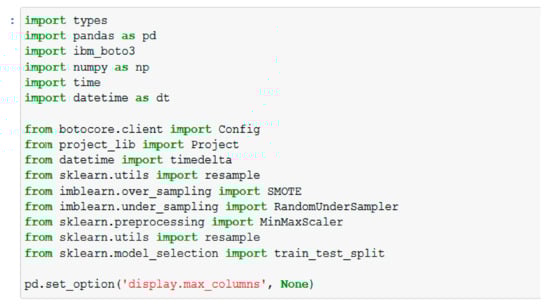
Figure 3.
Import packages.
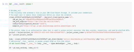
Figure 4.
Data generated by using ‘Insert to code’ function.
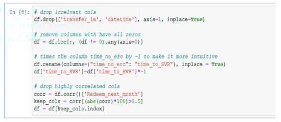
Figure 5.
Data cleaning.
In order to estimate the performance of ML models regarding the prediction of data that are not used for model training, the train-test split will be used (Figure 6). The first notebook, created for data preparation, started with importing the libraries and packages that will later be used (Figure 7) and adding the data by using the ‘Insert to code’ function. The code in Figure 8 was automatically generated.
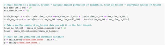
Figure 6.
Split train and test.
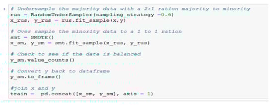
Figure 7.
Undersample and oversample.
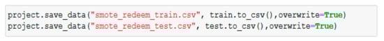
Figure 8.
Save the test and train datasets to Cloud Object Storage.
After importing the data, the next step is data cleaning. Firstly, the irrelevant columns have been dropped, continuing with removing the columns that have all zeros, multiplying the column ‘time_no_erc’ by −1 to make it more intuitive and dropping highly correlated columns. If two or more columns are extremely correlated, the chance is that at least one of them will not be chosen in a tree column sample and the tree will only depend on the remaining column(s). The corr() method from the pandas data frame has been used in order to remove the correlated features. The method returns a correlation matrix containing correlations with the column ‘Redeem_next_month’.
The train/test procedure is a method for estimating the performance of a machine learning algorithm. The split into train-test involves adjusting the dataset and diving it in two subsets: the training dataset that is used to fit the model and the testing dataset that is used to test the accuracy of the model. The train_test_split() method from the pandas data frame splits arrays or matrices into random train and test subsets. The size of the test array is selected through the method parameter ‘test_size’. The most common train/test split is 80/20, which means that 80% of the data will be for training while the rest of the 20% for testing.
As a part of data preparation, before splitting the training set into predictor and dependent variables, the records are split into two datasets, the ‘hotspot’ dataset that contains the highest proportion of redemption and the ‘train_no_hotspot’ dataset that contains everything that was left outside of the hotspot (Figure 9). A small sample of ‘train_no_hotspot’ dataset is added to the ‘hotspot’ dataset, the last step being splitting that final dataset into the predictor and dependent variables.
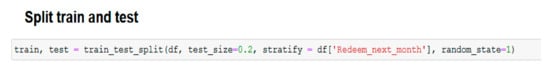
Figure 9.
Split records intro hotspot and no_hotspot datasets.
Imbalanced datasets are those datasets in which the distribution can be very disproportionate between the minority and the majority class. The bias in the training dataset can impact several machines learning algorithms, resulting with some of them completely ignoring the minority class. One of the best approaches to handle this issue with class imbalance is to resample the training dataset randomly. First step is to delete examples from the majority class, called under-sampling and then to duplicate example for the minority class, called oversampling. The randomly under-sample technique implemented on the majority class is RandomUnderSampler (). The second step is to handle the minority class. One way to oversample the minority class is to duplicate the examples from the minority class prior to fitting the model. Although this will balance the class distribution, it will not offer any supplementary information to the model. An upgrading to randomly duplicating the examples is to produce new examples from the minority class. The most commonly used approach to produce new examples is called SMOTE—Synthetic Minority Oversampling Technique. Nitesh Chawla et al. [53] describe this technique combined with under-sampling as having better results than simple under-sampling. “SMOTE first selects a minority class instance a at random and finds its k nearest minority class neighbours. The synthetic instance is then created by choosing one of the k nearest neighbours b at random and connecting a and b to form a line segment in the feature space. The synthetic instances are generated as a convex combination of the two chosen instances a and b.” [54].
The last step in the data preparation part of the project is to save the test and train datasets to Cloud Object Storage.
The second notebook begins with importing the necessary libraries (Figure 10) and importing the datasets created and saved in the previous notebook (Figure 11).
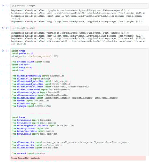
Figure 10.
Import libraries.
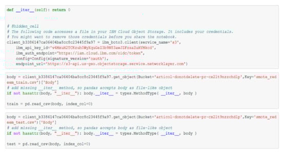
Figure 11.
Import data.
Both the train and the test datasets are split in 2 subsets (Figure 12): X_train, X_test that will contain all the independent features and y_train, y_test that will contain the dependent variables.
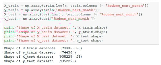
Figure 12.
Split datasets into train and test.
The following parts of the notebook consist in training several models to see which ones have the best results for the dataset imported. For all the models, hyper parameter tuning was done in order to obtain the best possible results.
In Figure 13, Figure 14, Figure 15 and Figure 16 the Random Forest hyperparameter tuning model is applied. In the Table 5, we have centralized the test results for each ML technique applied on the data set. The results in the table are supported by the outputs in the Appendix A.
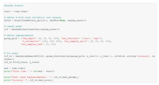
Figure 13.
Random Forest hyper parameter tuning.
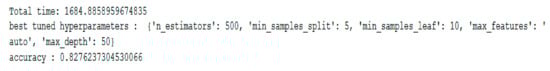
Figure 14.
Random Forest hyper parameter tuning results.
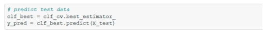
Figure 15.
Predicting test data.
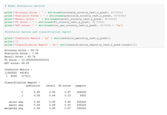
Figure 16.
Calculating the evaluation metrics and the confusion matrix.
Table 5.
The tests results for ML technique applied on the data set.
A first measure of the model’s performance is to test its accuracy. It is calculated as the ratio between the predicted correct observation and the total observations. In order to evaluate the performance of each proposed model, its accuracy was calculated. The higher the accuracy, the better the model is considered. There is also a limitation to accuracy testing. If there are no symmetric data sets in the data set in which the false positive and false negative values are approximately the same as the data volume, then accuracy is not considered a good measure for evaluating model performance [54,55].
In terms of accuracy, the best value is obtained for LightGBM model, followed by models XGBoost and random forest.
Another measure for performance testing is the Precision Score that is calculated as the ratio between the correctly anticipated positive observations and the predicted total positive observations. A high precision score value indicates a low false positive rate, i.e., when the predicted situation approaches the current situation. For our models, the highest value is obtained for the XGBoost model, followed by LightGBM and random forest models [56].
The next measure for evaluating the performance of the models is the Recall Score, which refers to the sensitivity between the correctly predicted positive observations and all real observations. It is considered that a value higher than 0.5 indicates a good performance of the model from the perspective of sensitivity of observations. From this point of view, the best models are AdaBoost and naïve Bayes [56,57].
Since we cannot draw a conclusion regarding the identification of the best performing models, we will also use the F1 Score measure which is calculated as a weighted average for Precision and Recall. The best values are obtained for XGBoost, random forest, and LightGBM models.
To understand AUC (area under the curve), the ROC curve must be explained. This is a graphical representation that projects the trade-off between the true positive rate and the false positive rate.
AUC ranges in value from 0 to 1. If the chosen model has 100% wrong predictions, AUC will take the value 0. If the model predictions are 100% correct, AUC will take the value 1 [57,58].
7. Conclusions
The influences of machine learning techniques in the evaluation of the life cycle of the mortgage loan product are of great complexity and with an impact on all loan products.
Comparing the results obtained with the ML algorithms (including those in the annex), the best results in terms of accuracy, precision, and validation were observed with random forest, XGBoost, and LightGBM. After preparing the data and applying the model over it, the accuracy scores as well the rest of the evaluation metrics have had very good results, denoting that the possibility of predicting the redemption of a client from a certain product are very high. Having the ability to predict the redemption will have a great impact, adding value to the bank’s planning. This type of prediction can be valuable not only to a bank, but to many more industries.
Based on the analyses performed, we can draw the following conclusions described in detail:
- (1)
- Compared to the existing empirical models that take into account only the application variables, the ML-based models also take into account the behavioral variables.
- (2)
- (3)
- The realization of this study offers different perspectives for future studies with impact on credit and credit risk models. In Romania, most banking institutions use internal risk models and traditional approaches in assessing the life cycle of a credit product.
Living in an age of data science and the rise of big data approaches such as machine learning or deep learning play a very important role in shaping credit risk today. The need for banks to adapt to this digital age with a huge volume of data is imperative. In this research we showed the importance of using automatic and deep learning techniques to verify the quality of data from a credit risk model related to the mortgage loan and its evolution of the life cycle. Like any microeconomic system, the commercial bank has a cybernetic system structure, in which the subsystems are distinguished, along with the relations between them, the connections with other systems in the environment, the system limits, and the feedback loops of internal regulation and adaptation to the environment. In general, the subsystems of a commercial bank can be classified into five components: credit management, deposits, risks, the funds insurance subsystem, and the treasury subsystem. From our point of view, credit and risk management is the most sensitive and important couple in the bank. Thus, in the future research, we will approach the commercial bank from the perspective of a complex, adaptive cybernetic system and we will apply machine learning techniques for the prediction of risk models and their validation.
The results of the case study show that the use of machine learning techniques reduces the implicit losses and ensures a high accuracy in predicting credit risk models. In addition, it can accelerate the digitization of banking institutions and can maintain a balance between the social ratio and that of reducing credit risk.
The need to understand human behavior in the current context has increased, regardless of the field analyzed. Thus, the understanding of behavioral economics is a topic of major interest in the context in which the influences related to the behavior of a system, an economic unit or any other actor in a system affect both micro and macro. For Romanian banks, the year 2020 will be a difficult one. Indeed, official estimates suggest that up to 12% of banks could record losses in the current financial year, profitability per customer being reduced by about 60% compared to 2019 [59]. Although most banks are studying internal and research to see what their customers want, there are also unanswered questions. Due to the importance that long-term customer loyalty has to the business banking institutions, the analysis and understanding of customer behavior is a key component of any analysis, thus allowing the bank to anticipate the likely reactions of customers, as well as to influence the structure of products and services offered.
By the nature of the activity of banking institutions and in the context of current competition, it becomes it is necessary to orient them, first of all, towards maintaining the existing, objective clients achievable by meeting customer satisfaction requirements and only subsequently, towards attracting to others. At the same time, maintaining a healthy loan portfolio is another goal of banks. These things can be improved by using machine learning techniques, a fact demonstrated in this research.
Author Contributions
Conceptualization, I.N., D.B.A., S.L.P.C. and Ș.I.; data curation, I.N., D.B.A., and Ș.I.; formal analysis: I.N.; investigation: I.N., D.B.A., S.L.P.C. and Ș.I.; methodology, I.N.; software, D.B.A. and I.N.; super-vision, I.N.; validation, I.N. and S.L.P.C.; visualization, D.B.A., S.L.P.C. and Ș.I.; writing—original draft, I.N., D.B.A. and S.L.P.C.; writing—review and editing, I.N. and Ș.I.; All authors have read and agreed to the published version of the manuscript.
Funding
This research received no external funding.
Institutional Review Board Statement
Not Applicable.
Informed Consent Statement
Not Applicable.
Data Availability Statement
Not Applicable.
Conflicts of Interest
The authors declare no conflict of interest.
Appendix A

Figure A1.
XGBoost hyper parameter tuning.

Figure A2.
Predicting test data.

Figure A3.
Calculating the evaluation metrics and the confusion matrix.

Figure A4.
LightGBM hyper parameter tuning.

Figure A5.
LightGBM hyper parameter tuning results.

Figure A6.
Predicting test data.

Figure A7.
Calculating the evaluation metrics and the confusion matrix.
References
- INSSE, National Strategy for the Sustainable Development of Romania Horizons 2013–2020–2030. Available online: https://insse.ro/cms/files/IDDT2012/StategiaDD.pdf (accessed on 20 February 2021).
- Communication from the Commission to the European Parliament, the Council, The European Economic and Social Committee and the Committee of the Regions. Available online: https://eur-lex.europa.eu/legal-content/EN/TXT/?uri=COM%3A2016%3A739%3AFIN (accessed on 20 February 2021).
- Burkhanov, U. The Big Failure: Lehman Brothers’ Effects on Global Markets. Eur. J. Bus. Econ. 2011. [Google Scholar] [CrossRef][Green Version]
- Ștefănescu-Mihăilă, R. Social Investment, Economic Growth and Labor Market Performance: Case Study-Romania. Sustainability 2015, 7, 2961–2979. [Google Scholar] [CrossRef]
- Nica, I. Simulation of financial contagion effect using NetLogo software at the level of the banking network. Theor. Appl. Econ. 2020, 2020, 55–74. [Google Scholar]
- Davies, H.; Green, D. Banking of the Future: The Fall and Rise of Central Banking; Princeton University Press: Princeton, NJ, USA, 2010. [Google Scholar]
- Thuiner, S. Banks of the Future. Putting a Puzzle Together Creatively; Springer: London, UK, 2015. [Google Scholar]
- Aniceto, M.; Barboza, F.; Kimura, H. Machine learning predictivity applied to consumer creditworthiness. Future Bus. J. 2020, 6. [Google Scholar] [CrossRef]
- BIS, Bank for International Settlements Working Papers. Available online: https://www.bis.org/publ/work834.pdf (accessed on 20 February 2021).
- Mital, A.; Varshneya, A. Reshaping Consumer Lending with Artificial Intelligence. Tavant Technologies. Available online: https://www.tavant.com/sites/default/files/download-center/Tavant_Consumer_Lending_Artificial_Intelligence_Whitepaper.pdf (accessed on 20 February 2021).
- Carbo-Valverde, S.; Cuadros-Solas, P.; Rodríguez-Fernández, F. A Machine Learning approach to the digitalization of bank customers: Evidence from random and causal forests. PLoS ONE 2020, 15, e0240362. [Google Scholar] [CrossRef]
- Addo, P.M.; Guegan, D.; Hassani, B. Credit Risk Analysis Using Machine and Deep Learning Models. Risks 2018, 6, 38. [Google Scholar] [CrossRef]
- Sirignano, J.A.; Sadhawani, A.; Giesecke, K. Deep Learning for Mortgage Risk. 2015, Cornell University. Available online: https://arxiv.org/pdf/1607.02470.pdf (accessed on 20 February 2021).
- Yu, Y.; Nguyen, T.; Li, J.; Sanchez, L.; Nguyen, A. Predicting elastic modulus degradation of alkali silica reaction affected concrete using soft computing techniques: A comparative study. Elsevier 2020. [Google Scholar] [CrossRef]
- Aggarwal, C.C. Neural Networks and Deep Learning; Springer International Publishing AG: Cham, Switzerland, 2018. [Google Scholar]
- Gennatas, E.D.; Friedman, J.H.; Ungar, L.H.; Pirracchio, R.; Eaton, E. Expert-Augmented Machine Learning. arXiv 2019, arXiv:1903.09731. [Google Scholar] [CrossRef]
- Géron, A. Hands-on Machine Learning with Scikit-Learn and Tensorflow: Concepts, Tools, and Techniques to Build Intelligent Systems; O’Reilly Media, Inc.: Sebastopol, CA, USA, 2017. [Google Scholar]
- Scarlat, E.; Chirita, N. Cibernetica Sistemelor Economice, 3rd ed.; Economica: Bucharest, Romania, 2019; ISBN 978-973-709-759-0. [Google Scholar]
- Goodman, L.S.; Li, S.; Lucas, D.J.; Zimmerman, T.A.; Fabozzi, F.J. Overview of the Nonagency Mortgage Market. In Subprime Mortgage Credit Derivatives; John Wiley & Sons, Inc.: Hoboken, NJ, USA, 2008; pp. 9–18. [Google Scholar]
- Hitchner, J.R. Financial Valuation. Applications and Models. In Introduction to Financial Valuation, 2nd ed.; John Wiley & Sons, Inc.: Hoboken, NJ, USA, 2006. [Google Scholar]
- Chorafas, D.N.; Steinmann, H. Expert Systems in Banking, A Guide for Senior Managers; Macmillan Academic and Professional LTD: Basingstoke, UK, 1991. [Google Scholar]
- Nica, I.; Chirita, N.; Scarlat, E. Approaches to financial contagion in the banking network. In Theory and Case Studies; Lambert Academic Publishing: Beau Bassin-Rose Hill, Mauritius, 2020; ISBN 978-620-2-91797-1. [Google Scholar]
- Hill, D.; Mitter, S. Cybernetics or Control and Communication in the Animal and the Machine, Reissue of the 1961 Second Edition, Norbert Wiener; The MIT Press: London, UK, 2019. [Google Scholar]
- Kline, R. The Cybernetics Moment or Why We Call Our Age the Information Age; Johns Hopkins University Press: Baltimore, MD, USA, 2015. [Google Scholar]
- Wiener, N. Cybernetics or Control and Communication in the Animal and the Machine, 2nd ed.; MIT Press: London, UK, 1965. [Google Scholar]
- Parra-Luna, F. Systems Science and Cybernetics; Eolss Publishers/UNESCO: Oxford, UK, 2009. [Google Scholar]
- Miller, J.H.; Page, S.E. Complex Adaptive Systems: An introduction to Computational Models of Social Life; Princeton University Press: Princeton, NJ, USA, 2007. [Google Scholar]
- Nilsson, N.J. Introduction to Machine Learning; Department of Computer Science, Stanford University: Standford, CA, USA, 1996. [Google Scholar]
- Kodratoff, Y.; Paliouras, G.; Karkaletsis, V.; Spyropoulos, C.D. Machine Learning and Its Applications; Springer: Berlin/Heidelberg, Germany, 2001. [Google Scholar]
- Mitchell, T.M. Machine Learning; McGraw-Hill Science/Engineering/Math: Portland, OR, USA, 1997. [Google Scholar]
- Harrington, P. Machine Learning in Action; Manning Publications: Shelter Island, NJ, USA, 2012. [Google Scholar]
- Touw, W.; Bayjanov, J.; Overmars, L.; Backus, L.; Boekhorst, J.; Wels, M.; van Hijum, S. Data mining in the Life Sciences with Random Forest: A walk in the park or lost in the jungle? Brief. Bioinform. 2013, 14, 315–326. [Google Scholar] [CrossRef]
- Verikas, A.; Gelzinis, A.; Bacauskiene, M. Mining data with random forests: A survey and result of new tests. Pattern Recognit. 2011, 44, 330–349. [Google Scholar] [CrossRef]
- Denisko, D.; Hoffman, M. Classification and interaction in random forests. Proc. Natl. Acad. Sci. USA 2018, 115. [Google Scholar] [CrossRef]
- Breiman, L. Random Forests. Mach. Learn. 2001, 45, 5–32. [Google Scholar] [CrossRef]
- Morgan, J.N.; Sonquist, J.A. Problems in the Analysis of Survey Data, and a Proposal. J. Am. Stat. Assoc. 2012, 58, 415–434. [Google Scholar] [CrossRef]
- Carmona, P.; Climent, F.; Momparler, A. Predicting failure in the U.S. banking sector: An extreme gradient boosting approach. Int. Rev. Econ. Financ. 2019, 61, 304–323. [Google Scholar] [CrossRef]
- Ibrahem Ahmed Osman, A.; Najah, A.A.; Chow, M.; Feng, H.Y.; El-Shafie, A. Extreme gradient boosting (Xgboost) model to predict thegroundwater levels in Selangor Malaysia. Ain Shams Eng. J. 2021. [Google Scholar] [CrossRef]
- Dhieb, N.; Ghazzai, H.; Besbes, H.; Massoud, Y. Extreme Gradient Boosting Machine Learning Algorithm for Safe Auto Insurance Operations. In Proceedings of the 2019 IEEE International Conference on Vehicular Electronics and Safety, Cairo, Egypt, 4–6 September 2019. [Google Scholar] [CrossRef]
- Machado, M.; Karray, S.; de Sousa, I. LightGBM: An Effective Decision Tree Gradient Boosting Method to Predict Customer Loyalty in the Finance Industry. In Proceedings of the 14th International Conference on Computer Science & Education (ICCSE), Toronto, ON, Canada, 19–21 August 2019. [Google Scholar]
- Creamer, G.; Freund, Y. Using Boosting for Financial Analysis and Performance Prediction: Application to S&P 500 Companies, Latin American ADRs and Banks. Comput. Econ. 2010, 36, 133–151. [Google Scholar] [CrossRef]
- Chopra, A.; Bhilare, P. Application of Ensemble Models in Credit Scoring Models. Bus. Perspect. Res. 2018, 6, 227853371876533. [Google Scholar] [CrossRef]
- Momparler, A.; Carmona, P.; Climent, F. Banking failure prediction: A boosting classification tree approach. Span. J. Financ. Account. Rev. Española Financ. Contab. 2016, 45. [Google Scholar] [CrossRef]
- Annin, K.; Omane-Adjepong, M.; Sarpong Senya, S. Applying Logistic Regression to E-banking usage in Kumasi Metropolis, Ghana. Int. J. Mark. Stud. 2014, 6. [Google Scholar] [CrossRef]
- Krichene, A. Using a naive Bayesian classifier methodology for loan risk assessment: Evidence from a Tunisian commercial bank. J. Econ. Financ. Adm. Sci. 2017, 22, 3–24. [Google Scholar] [CrossRef]
- Abdelmoula, A.K. Bank Credit Risk Analysis with K-Nearest-Neighbor Classifier: Case of Tunisian Banks. J. Account. Manag. Inf. Syst. Fac. Account. Manag. Inf. Syst. Buchar. Univ. Econ. Stud. 2015, 14, 79–106. [Google Scholar]
- Research Gate, Hyperparameter Tuning. Available online: https://www.researchgate.net/publication/335491240_Hyperparameter_Tuning (accessed on 20 February 2021).
- Probst, P.; Bischl, B.; Boulesteix, A.-L. Tunability: Importance of Hyperparameters of Machine Learning Algorithms. J. Mach. Learn. Res. 2019, 20, 1–32. [Google Scholar]
- Research Gate, Hyperparameter Tuning. In Project: Application of Population Based Algorithm on Hyperparameter Selection. Available online: https://www.researchgate.net/publication/340720901_Hyperparameter_Tuning (accessed on 20 February 2021).
- Probst, P.; Wright, M.; Boulesteix, A.-L. Hyperparameters and Tuning Strategies for Random Forest. Wiley Interdiscip. Rev. Data Min. Knowl. Discov. 2019, 9. [Google Scholar] [CrossRef]
- Haghighi, S.; Jasemi, M.; Hessabi, S.; Zolanvari, A. PyCM: Multiclass confusion matrix library in Python. J. Open Source Softw. 2018, 3, 729. [Google Scholar] [CrossRef]
- Miller, J. Hands-On Machine Learning with IBM Watson: Leverage IBM Watson to Implement Machine Learning Techniques and Algorithms Using Python; Packt Publishing: London, UK, 2019. [Google Scholar]
- Chawla, N.V.; Bowyer, K.W.; Hall, L.O.; Kegelmeyer, W.P. ‘SMOTE: Synthetic Minority Over-sampling Technique’. J. Artif. Intell. Res. 2002, 16, 321–357. [Google Scholar] [CrossRef]
- Haibo, H.; Yunqian, M. Imbalanced Learning: Foundations, Algorithms, and Applications; Wiley: Hoboken, NJ, USA, 2013. [Google Scholar]
- Kulkarni, A.; Chong, D.; Batarseh, F. Foundation of Data Imbalance and Solutions for a Data Democracy; Elsevier, Data Democracy: Amsterdam, The Netherlands, 2020; pp. 83–106. [Google Scholar]
- Accuracy, Precision, Recall & F1 Score: Interpretation of Performance Measures. Available online: https://blog.exsilio.com/all/accuracy-precision-recall-f1-score-interpretation-of-performance-measures/ (accessed on 30 March 2021).
- F1 Score vs ROC AUC vs Accuracy vs PR AUC: Which Evaluation Metric Should You Choose? Available online: https://neptune.ai/blog/f1-score-accuracy-roc-auc-pr-auc (accessed on 30 March 2021).
- Classification: ROC Curve and AUC. Available online: https://developers.google.com/machine-learning/crash-course/classification/roc-and-auc (accessed on 30 March 2021).
- Economia HotNews. Available online: https://economie.hotnews.ro/stiri-finante_banci-24234743-cum-schimbat-pandemia-relatia-banca-marile-necunoscute-ale-bancilor-privire-comportamentul-asteptarile-clientilor.htm (accessed on 31 March 2021).
Publisher’s Note: MDPI stays neutral with regard to jurisdictional claims in published maps and institutional affiliations. |
© 2021 by the authors. Licensee MDPI, Basel, Switzerland. This article is an open access article distributed under the terms and conditions of the Creative Commons Attribution (CC BY) license (https://creativecommons.org/licenses/by/4.0/).