Construction Sector Contribution to Economic Stability: Malaysian GDP Distribution

Abstract

The construction sector exerts an exceptional impact on economic development all over the world. Adequate buildings and infrastructures made by the construction sector ensure that a country reaches certain targets like social development, industrialization, freight transportation, sustainable development, and urbanization. This study aims to determine the construction sector’s connectivity with other sectors through complex linkages that contribute immensely to the economy and gross domestic product (GDP). The data were collected from the Department of Statistics Malaysia and the World Bank from the year 1970 to 2019, and the Pearson correlation test, the cointegration test, and the Granger causality test were conducted. The vector error correction model (VECM) was created for short-term and long-term equilibrium analysis and impulse response function (IRF) was performed to study construction industry behavior. Afterwards, the forecasting was done for the year 2020 to 2050 of the Malaysian economy and GDP for the required sectors. It was revealed that some sectors, such as agriculture and services, have forward linkages while other sectors, such as manufacturing and mining, are independent of construction sector causality, which signifies the behavior of the contributing sectors when a recession occurs, hence generating significant revenue. The Malaysian economy is moving towards sustainable production with more emphasis on the construction sector. The outcome can be used as a benchmark by other countries to achieve sustainable development. The significance of this study is its usefulness for experts all over the world in terms of allocating resources to make the construction sector a sustainable sector after receiving a shock. A sustainable conceptual framework has been suggested for global application that shows the factors involved in the growth of the construction industry to ensure its sustainable development with time.

1. Introduction

A country’s prosperity is linked to its economic growth where all the sectors, such as primary, secondary, tertiary, and quaternary sectors, contribute to stabilizing the economy [1,2]. The construction sector has prime importance that signifies the prosperity, health, and quality of life for the country’s citizens [3,4]. The construction sector acts as a backbone of the economic growth of any country, therefore, it influences every sector’s role on all levels in an economy [5,6]. Developing countries are mostly dependent on the construction sector to implement their sustainable development [7,8]. The construction sector exerts a direct influence on social and economic development in money circulation [9]. Therefore, the absence of adequate building infrastructure results in undergrowth of a country’s sectors, an underdeveloped economy, a substandard level of living, and imbalanced income distribution, which are the contributing factors towards a country’s economic failure [10,11]. The effective management of the construction sector results in improved life quality, including boosted tourism, sustainable environment, money circulation, and job creation throughout the country [12,13]. In the economy, the gross domestic product (GDP) plays a vital role in balancing various sectors. Overall, the construction sector accounts for USD 1.7 trillion worldwide, and in most countries, it impacts 5–7% of the total GDP [14]. The construction sector contributes significantly to the national GDP, thus the need for development in this sector is important [15].

It has been reported that most countries are investing in research and development (R&D) to develop sustainable techniques for the construction sector [16]. Hence, revolutionizing the construction sector will ensure sustainable development [17]. Any variation in the construction sector will have a direct influence on all the related sectors [12,18,19]. The construction sector has a significant role in the economy, therefore, its influence in a country’s economy is associated with forward and backward linkages with other sectors [17]. These linkages with other sectors are dependent on performance, therefore, a change in any of the sectors will have significant repercussions on the country’s economy [20]. Thus, the construction sector has a considerable influence on the socio-economic aspects of any nation [21].

It is estimated that one-third of countries depend on resources which are necessary for social and economic development [22,23]. However, establishing sustainable goals does not require a significant workforce or abundance of resources, rather, it requires technological innovation, resourceful use of the materials, and smart industrial processes in developing and developed countries [24]. In developing countries, the construction sector is greatly influenced by globalization, as most of the complex, innovative techniques, and skilled manpower required for sustainable development are not available in the local market, therefore, they have to depend on the inescapable fact of globalization [25]. Most developed countries have norms that are no different from those of others, for example, in the construction sector, most practices in developing countries are influenced by the practices followed in developed countries [26]. Therefore, the conventional method of construction is still in effect in commonwealth countries [27,28].

The Malaysian construction sector (MCS) is facing various problems, like shortages of manpower, environment solutions, quality of the work, and a dearth of productivity, which have raised many challenges [29,30]. One of the contributing factors that hinders the performance of the construction sector in Malaysia is the conventional construction approach. The country must shift to modern construction technology like Hong Kong, Singapore, and the United Kingdom (UK) [31]. There is an absence of a framework to enhance the competitiveness, resource allocation, and funding laws, hence the quality level decreases in the national and international market [32]. The new challenges that the MCS is facing are: slow progress in terms of sustainability, excessive and unregularized use of resources, the absence of construction techniques causing less pollution, and energy efficiency [30]. The R&D for the construction sector in Malaysia is mostly carried out by educational institutes, which is not scalable to practical uses as per construction requirements [33]. The lack of a fair bidding process and transparent tendering [34] and the failure of timely release of funding [35] have contributed considerably to the underperformance of the MCS. The minimum growth of overall GDP was recorded in quarter (Q)1’2019 at just RM 341.6 billion as compared to the maximum of RM 3701 billion in Q4’2019. The percentage change shows a maximum growth of the Malaysian economy in Q3’2017, while from Q1’2016 to Q3’2019, there was not such a significant change in the percentage of overall GDP. However, a considerable fall in GDP production in Q1’2020 and Q2’2020 occurred because of the lockdown situation due to COVID-19, with a reduction of 17.1% in Q2’2020, whereas in Q3’2020, a reduction percentage was recorded as being 2.7% [36].

However, it should be noted that unseen events like the COVID-19 outbreak can significantly affect the performance of the overall GDP as well as the contributing sectors. The overall GDP began to crumble as COVID-19 started to show its effects. For comparison purposes, it is evident that the Malaysian economy grew 3.6% in Q4’2019. With the effect of lockdown in Malaysia after the first case of COVID-19 was reported, there was a fall in the major sector of construction (CONST) and other sectors like services (SERV), manufacturing (MANU), agriculture (AGRI), and mining (MINI) in Q1’2020, but the effects were not quick as there was a surplus of material available in all sectors. The situation got worse when the COVID-19 outbreak was prolonged and people were forced to stay in their homes, which showed its repercussions in Q2’2020. With the prolonged lockdown, there was a major decrease in the Malaysian economy, as it contracted to 17.1% in Q2’2020 due to the fall in construction GDP to 44.5%. Hence, it is clear that the suspension of the construction industry is a major threat to the stability of the economy. At the end of Q3’2020, the economy saw a smaller decline of 2.7% in the overall GDP of all the sectors. In general, the effects of COVID-19 were not present in Q4’2019. The values are shown in

Table 1. Sector-wise quarterly gross domestic product (GDP) of Malaysia.

Sector	GDP in Q4’2019	GDP in Q1’2020	GDP in Q2’2020	GDP in Q3’2020
Construction	1.0%	−7.9%	−44.5%	12.4%
Services	6.1%	3.1%	−16.2%	−4.0%
Manufacturing	3.0%	1.5%	−18.3%	3.3%
Agriculture	−5.7%	−8.7%	1.0%	−0.7%
Mining	−2.5%	−2.0%	−20.0%	−6.8%

[37,38,39].

The above table shows the construction sector in comparison with the other sectors because the construction sector is considered as the major sector of Malaysian GDP and it has considerable volatility in the economy, therefore, MCS analysis was essential.

In Malaysia, the highest value of construction work was recorded in 2019, at approximately RM 146.37 billion. The value of construction work increased annually by approximately RM 10 billion from 2012 to 2018 [40]. There is not much difference between the value of construction work in 2018 and 2019 because the Malaysian government suspended construction activity to decrease debt. Since the classification of COVID-19 as a pandemic by the World Health Organization (WHO), most countries prepared for nationwide lockdown, which disrupted the economy, social life, and caused the shutting down of businesses. Among other sectors, the construction sector was also affected, which resulted in financial implications, overrunning of costs, halted projects, delays in projects, and loss of jobs [41]. Therefore, this research focused on studying the effects of shocks on the construction industry and what short- and long-term policies have to be applied to optimize the social and economic sustainability in the region. Moreover, this study also provides an essential sustainable framework as a guideline for international applications in order to establish a sustainable construction industry. Due to such importance, the following research questions were established:

• In which direction does the construction industry move to recover from external shocks and the time taken to regain its original position?
• What short- and long-term policies and decisions will affect the behavior of construction to achieve sustainability?
• What sustainable framework should be followed to achieve sustainability in the construction industry that has global application?

The Granger causality test was used to assess the direction of the shock, which was produced using the impulse response function (IRF). The short- and long-term policies were assessed after creating a system of equations using the vector error correction model (VECM). A sustainable framework was proposed based on the results of the IRF and VECM along with its international applicability. The fundamental objective of conducting this study was to assess the role of the MCS in the prosperity of the Malaysian economy and how any change in the growth of the construction sector would impact the behavior of other sectors. This study addressed the issue of how much would the MCS be impacted when there is a unit investment in other sectors and vice versa, and what long-term actions the government should take to make the industry sustainable. The answer to this question was found by using the identification of the linkage direction of the MCS and use of the VECM equation by introducing a shock to study MCS behavior and assess the time required to fully recover from any shock, like a recession or lack of investment. Additionally, a conceptual framework was proposed to guide the governments of their respective countries about the necessary steps that they should take to make the construction sector shockproof or sustainable. Forecasting was performed to predict the sustainability of the construction sector if the present condition prevailed in the MCS. The application of unit shocks has never been tested in the construction sector which could move it one step closer towards its goal to attain sustainability in the region. This study is beneficial in terms of defining the socio-economical guidelines for the MCS to estimate the linkage model with other sectors. The financial planners and policymakers of Malaysia can use the results of this study to improve the construction sector by using advanced strategies, thus enabling Malaysia to be a progressive and prosperous country by the year 2050.

2. Literature Review

Numerous studies have been conducted to study and highlight the issues that are faced by the construction sector. VECM, regression, and Box–Jenkins methods were used for analyzing and predicting the construction tender prices index (TPI) in the Hong Kong market. With the value of mean absolute percentage error (MAPE) as 2.9%, it was found that the VECM outperforms the other two methods in prediction in terms of short- and long-term price movements [42]. The data from Melbourne and Sydney were used to perform an econometric approach to study the short- and long-term construction prices and their direction in Australia using the VECM and Granger causality test, respectively. The linkages and diffusion patterns were found among six states and two territories. It was concluded that there exists one returning diffusion path for every territorial market, hence, the shares go back to the funding of the federal state [43]. The VECM, along with the Box–Jenkins method and regression analysis, were put into use to predict the construction prices. The models were evaluated using the predictive ability of Theil coefficients and MAPE with values of 0 and 10%, respectively. It was found that the VECM with the inclusion of dummy variables predicts the prices better than the other two models [44]. The data of construction demand were obtained from the Australian Bureau of Statistics for the period of Q3’1998 to Q4’2013. The VECM indicated the links between the construction sector and state prices, population, and unemployment. The MAPE value of the VECM was lowest among all the other models, which was less than 10%, indicating robust reliable forecasting [45]. The forecasting of the cost of highway construction was performed based on the data collected from the State Department of Transportation. The VECM illustrated that raw oil and construction costs fit the diagnostics tests better. The presence of multivariate variables significantly increased the accuracy of the results as compared to univariate forecasting using the VECM [46]. The prices of construction materials like cement, steel, and asphalt were forecasted based on the data of the United States of America (USA). The methodology of the VECM was employed for examining short- and long-term effects on the mentioned prices. Based on the lowest values of MAPE and Theil coefficients, the VECM with asphalt prices outperformed the other variables [47]. The demand for construction workers was forecasted based on the data of Q1’1983-Q3’2005 in Hong Kong. After using the VECM as the method of analysis, it was revealed that labor skill and construction output were the major factors that influence the employment opportunities in this sector [48]. The construction cost index (CCI) short- and long-term effects on the consumer price index were tested and forecasting was performed using the unrestricted vector autoregression (VAR) model. The model was found to accurately forecast the cost trends of construction based on the lowest values of the mean squared errors (MSEs) and the mean absolute errors (MAEs) [49]. The construction material prices were generated for long-term effects using regression methods and VAR. The method of forecasting indicated that the presence of autocorrelation and higher values of R² greatly affected the performance of VAR processes like the VECM [50]. A study was conducted based on data from 2001 to 2006 of China, and the real estate demand and construction demand were forecasted. Regression analysis and cointegrating vectors were used for the purpose of forecasting It was found that economic planning is the reason for the change in investments in the Chinese market [51]. Economic development in developing countries saw a considerable rise without paying any heed to sustainability, which resulted in global warming [52], increased CO₂ emissions [53], and the generation of hazardous waste emanating from construction machinery [52] and steel [54] and cement manufacturing [55]. Based on the literature, there is an absence of work proposing a sustainable framework for the construction sector. The current practices of the construction sector of Malaysia were assessed for their sustainability based on questionnaires and interviews. To enable the construction sector in Malaysia to be fully sustainable, three major principles, namely environmental, social, and economic development, are needed [56]. Sustainability in the Malaysian construction sector is not new. Every skilled worker of construction sector is well aware of the sustainable work protocols but they turn a blind eye due to its need of bigger workforce, initial high costs and little acceptability in the traditional construction methods and absence of strict legislation [57]. Currently, Malaysia is facing major problems regarding CO₂ emissions and sustainability, therefore, the inflation effects on CO₂ emission were assessed. It was revealed that due to the decrease in the rate of inflation, the construction sector flourished, however, this poses a threat to the environment and has negative consequences for sustainability. By following the proposed inflation rate and CO₂ framework, Malaysia can overcome this problem [58]. The need for sustainable construction in Malaysia will ensure less usage of resources, reduced production costs, and holistic management of wastes. The lack of government enforcement, tax exemptions, and low level of interest of stakeholders in investing in sustainable processes and proper frameworks of sustainability are the reasons that the Malaysian construction sector is lagging in sustainable construction processes [59].

3. Methodology

To summarize the methodological procedure, the acquired data were shaped into the same base price index of constant year 2015. Later, the Pearson correlation test, unit root test, optimal lag length, cointegration test, causality test, and vector error correction model (VECM) steps were conducted. Furthermore, the forecast for the MCS was performed from the year 2020 to 2050. This study adopts a quantitative approach where the forecasting was performed on collected data of the Malaysian economy. Econometric and descriptive analyses were performed simultaneously, which led to the conclusion.

3.1. Data Collection

The data collection of the contributions of the construction sector (CONST), agriculture sector (AGRI), manufacturing sector (MANU), service sector (SERVC), and mining sector (MINING) to GDP was done with the Department of Statistics Malaysia [60] and World Bank Statistics from the year 1970 to 2019 [61]. The reason for selecting these variables is that they are the major sectors of the Malaysian economy. Any change in these sectors will show its effect on the national GDP of Malaysia. The data are in local currency units (LCUs), i.e., in the constant year 2015, as presented in Appendix A.

3.2. Data Analysis

After the data collection, the Pearson correlation test was performed to find if any correlation exists among the sectors. Then, the augmented Dickey–Fuller (ADF) test was conducted to find the presence of the unit root. As the order of integration was the same, the VECM was applied. The Granger causality test was conducted to find the direction of the dependence of each sector. The VECM equation was obtained along with coefficient values. The IRF was used by giving a shock to the construction sector to find how other sectors behave. Finally, forecasting from the year 2020 to 2050 was performed.

3.2.1. Initial Tests for Conducting Analysis

To assess the strength of any two variables, the Pearson correlation test was performed by using Equation (1) between the MCS and other concerned sectors:

$$\mathrm{r}=\frac{n \left(\sum XY\right)-\left(\sum X\right)\left(\sum Y\right)}{\sqrt{\left[n \left(\sum X^2\right)-{\left(\sum X\right)}^2\right][n( \left(\sum Y^2\right)-{\left(\sum Y\right)}^2)}]}$$

(1)

where X and Y are the variables, n shows the number of observations, and r is the correlation coefficient.

For the determination of the presence of the unit root, the ADF test was used. The added advantage of the ADF test is that if a correct lag order is identified, the accuracy of the ADF test could be increased [62]. The mathematical form of the ADF test is given in Equation (2):

$$\mathsf{\Delta }{Y}_t={\alpha }_1+{\alpha }_{2}T+𝜏{\mathrm{Y}}_{t-1}+{\gamma }_i{\sum }_{t=1}^n\mathsf{\Delta }Y t_{-}{1}_{}+{\mu }_t$$

(2)

where Y_t is the time series, ΔYt = Y_t − Y₁, T is the trend with time, α is the drift term, μ_t is the error term, and n is the number of lags to capture the white noise [63].

3.2.2. Cointegration Tests

The linear relation of stationary time series data is called a cointegration model equation. This study used the Johansen cointegration test [64], which was developed by Johansen and Juselius [65]. This method was used to determine the relationship between the multidirectional time series. The null hypothesis was tested for a p-value of 0.05.

3.2.3. Pairwise Granger Causality

This test was first developed by Granger [66] and its underlying principle is that if a time series “X” can be used to estimate the time series “Y” past data, then the previous values of “X” have significant power to estimate the present “Y”, where “X” might be causing “Y” [67]. The mathematical form is shown in Equations (3) and (4):

$$Y_t={\beta }_0+{{\displaystyle \sum }}_{j=1}^J{\beta }_j{Y}_{t-j}+{{\displaystyle \sum }}_{k=1}^K{\gamma }_k{X}_{t-k}+{\mu }_t$$

(3)

$$X_t={\beta }_0+{{\displaystyle \sum }}_{j=1}^J{\beta }_j{X}_{t-j}+{{\displaystyle \sum }}_{k=1}^K{\gamma }_k{Y}_{t-k}+{\mu }_t$$

(4)

where ${\mu }_t$ is uncorrelated white noise, ${\gamma }_k$ is a measure of the influence of $X_{t-k}$ on $Y_t$. If ${\gamma }_k$ is statistically significant for both the equations, then causality is bidirectional.

3.2.4. Vector Error Correction Model (VECM)

The error correction model (ECM) is recommended when there is the presence of the unit root and the variables are cointegrated. The ECM is used to introduce short-term and long-term equilibrium adjustment mechanisms when the variables diverge from the equilibrium. When the direction of the variable is required, the ECM is changed into the VECM. The mathematical form was given by Gujarati [68] and Granger [69], which is provided in Equation (5):

$$\mathsf{\Delta }{Y}_t={\displaystyle \prod }{Y}_{t-1}+{{\displaystyle \sum }}_{i=1}^{m-1}{\Phi }_i\mathsf{\Delta }{Y}_{t-i}{D}_i+{\mu }_t$$

(5)

where ΔY_t is the independent variable, ∏ is the matrix of cointegrating vectors, Φ represents a matrix of independent variables [68]. VECM captured short-term and long-term effects among the variable of stock prices [70]. The reason this study used VECM as a method of analysis is because of its applicability in multivariate time series, secondly, more precise short-term and long-term interdependencies are obtained if the equations are cointegrated [71].

3.2.5. Cumulative Sum (CUSUM) Tests

This test was developed by Brown et al. [72] for structural stability, and the mathematical form is shown in Equation (6). The principle behind this test is that the model is tested for a structural break because the presence of a structural break in the unit root will lead to inaccurate results of the model [73].

$$w_m=\frac{1}{\widehat{\sigma }}{{\displaystyle \sum }}_{t=k+1}^T{w}_t,m=k+1,\dots ,t$$

(6)

where $w_t$ the recursive residual, m is the sample number. The analysis is rejected if the plot deviates from the suggested boundary by the test level of confidence of 95%.

3.2.6. Impulse Response Functions (IRFs)

The IRF usage in this study signifies how a dependent variable responds to the vector autoregressive (VAR) model when a standard deviation shock is introduced to the error parameter. This study uses the Cholesky degree of freedom (DOF) test [74].

3.2.7. Forecasting

The final step was forecasting, which was performed to check the future behavior based on the past values of the construction sector. The reason for conducting forecasting was to guide statisticians and the government in terms of the forthcoming rise or fall in the construction GDP. Based on the proposed framework and forecasting, the government can take preventive measures to naturalize the sector shock in less time. The model validation is based on the Theil coefficient, RMSE, and MAPE that ensure the goodness-of-fit of the VECM forecasted values.

4. Results and Discussion

4.1. Relationship between Sectors and Stationarity Determination

The relationship between the selected sectors of the Malaysian economy was analyzed based on the results of the Pearson correlation test, as shown in

Table 2. Pearson correlation test.

	CONST	AGRI	GDP	MANU	MINING	SERVC
CONST	1	-	-	-	-	-
AGRI	0.957372	1	-	-	-	-
GDP	0.979313	0.978232	1	-	-	-
MANU	0.968410	0.971241	0.99501	1	-	-
MINING	0.967215	0.968167	0.994983	0.998431	1	-
SERVC	0.980794	0.980149	0.99728	0.993659	0.990488	1

. The reason to include the GDP in the Pearson correlation test was to observe its fluctuation with the shock in the construction sector. The result shows that all the sectors are highly correlated with each other.

After the Pearson test, the unit root (ADF) test was used. As per the results, the unit root exists at the level intercept, as shown in

Table 3. Unit roots test (ADF) results.

Variable	Lag Order	t*	ADF Results	Order of Integration	Decision at Significance Level
LAGRI	4	2.922	6.40	I (1)	non-stationary
LMINING	4	2.923	6.22	I (1)	non-stationary
LMANU	4	2.923	6.95	I (1)	non-stationary
LGDP	4	2.923	5.76	I (1)	non-stationary
LSERVC	4	2.923	4.23	I (1)	non-stationary
LCONST	4	2.923	4.78	I (1)	non-stationary

t* = t-statistic critical value at various significance levels.

. On the basis of ADF results, the first difference with a p-value of 0.05 shows that the data is stationary and a single order of integration exists in the data. Therefore, the data are suitable for the analysis of causality, the VECM, the IRF, and forecasting. The value shows that there exists a long-term relationship between the variables.

If t* < ADF critical value, the null hypothesis is rejected, i.e., the unit root does not exist. The data are non-stationary at this level. After one difference, the data become stationary with t* < ADF, therefore, the order of integration was selected as I (1), which shows that the values are a good fit for analysis.

4.2. Optimal Lag Length

The lag length analysis was performed where a lag length of 4 was selected based on the lowest value of the Akaike information criterion (AIC), as shown in

Table 4. Lag length selection.

Lag	LR	FPE	AIC	SC	HQ
0	NA	4.73 × 10−12	−9.049402	−8.815502	−8.961011
1	648.5405	2.90 × 10−18 *	−23.36746	−21.73016 *	−22.74872 *
2	54.57443 *	2.93 × 10−18	−23.42673 *	−20.38603	−22.27765

* Indicates lag order selected by the criterion, LR = Sequential modified LR test statistic (each test at 5% level), FPE = Final prediction error, AIC = Akaike information criterion, SC = Schwarz information criterion and HQ = Hannan-Quinn information criterion.

. Based on the results, a lag order of 2 was selected, which was used for building the VECM.

4.3. Pairwise Granger Causality Analysis

Granger pairwise causality tests the null hypothesis that ARGI does not Granger cause CONST. If the value of Prob. is less than 0.05 (p-value < 0.05), the null hypothesis is rejected. The results show that AGRI Granger causes CONST. In the case of AGRI–CONST and SERVC–CONST, the null hypothesis was rejected as the change in CONST does have causal effects on AGRI. The same is the case with SERVC and CONST because the p-value is less than 0.05, as shown in

Table 5. Empirical results of Granger causality.

Null Hypothesis	Lag	Alternate Hypothesis	F-Stat	p-Value	Null Hypo Result
AGRI does not Granger Cause CONST	2	AGRI Granger causes CONS	4.775	0.013	Reject
CONST does not Granger Cause AGRI	2	-	0.610	0.547	Accept
GDP does not Granger Cause CONST	2	-	2.851	0.068	Accept
CONST does not Granger Cause GDP	2	-	1.853	0.169	Accept
MANU does not Granger Cause CONS	2	-	1.778	0.181	Accept
CONST does not Granger Cause MANU	2	-	0.474	0.625	Accept
MINI does not Granger Cause CONS	2	-	1.135	0.330	Accept
CONST does not Granger Cause MINI	2	-	0.859	0.430	Accept
SERV does not Granger Cause CONS	2	SERVC Granger causes CONST	4.159	0.022	Reject
CONST does not Granger Cause SERV	2	-	1.485	0.237	Accept

.

4.4. Linkage Direction

It is evident that unidirectional causality exists between AGRI and CONST, and SERV and CONST. There are three independent variables, namely GDP, MANU, and MINI. There are no bidirectional linkages between any other sectors, as shown in

Table 6. Direction of linkage.

Description	Direction of Linkages
Agriculture and Construction	Unidirectional (Agriculture to Construction)
GDP and Construction	Independent
Manufacturing and Construction	Independent
Mining and Construction	Independent
Services and Construction	Unidirectional (Services to Construction)

.

4.5. Johansen–Jusilus Cointegration Examination

The null hypothesis was tested, which states that no cointegrating equations existed, which was rejected for the first two equations based on the p-values being less than 0.05, as shown in

Table 7. Unrestricted cointegration rank test (maximum eigenvalue).

Hypothesized No. of Cointegrating Eqn(s)	Eigenvalue	Max-Eigen Statistic	0.05 Critical Value	p-Value
None *	0.730538	61.63243	40.07757	0.0001
At most 1 *	0.527047	35.19165	33.87687	0.0347
At most 2	0.420552	25.64697	27.58434	0.0867
At most 3	0.317081	17.92481	21.13162	0.1327

* Max-eigenvalue test indicates 2 cointegrating eqn(s) at the 0.05 level.

. The null hypothesis was rejected at a p-value of 0.05 and the number of equations selected for analysis was two.

If the variables are not cointegrated (have a long-term relationship), then unrestricted VAR is used for analysis. If the variables are cointegrated, then the usage of restricted VAR is preferred, i.e., the VECM.

4.6. VECM for Construction Sector

The VECM performs better while observing the short- and long-term causality through the estimated variables. The proposed relationship of this study is given in Equation (7):

CONST = ƒ (AGRI, CONST, GDP, MANU, MINING, SERVC)

(7)

Equation (7) was generated by the VECM for short- and long-run equilibria. The model equation consists of two major parts, namely cointegrating equations and error correction mechanisms, which show the speed of adjustment that the sector will undergo to come back to its original state. The latter indicates the short-run coefficients’ causality among the variables, which is represented by Equation (8):

D(LCONST) = C(1) × (LCONST(−1) + 1.67180917629 × LMINING(−1) − 2.68403475444 × LSERVC(−1) + 0.941037693325 × LGDP(−1) – 3.78428477371) + C(2) × (LAGRI(−1) − 1.86519424503 × LMINING(−1) + 9.43226731209 × LSERVC(−1) – 10.9476629704 × LGDP(−1) + 24.4605216091) + C(3) × (LMANU−1) − 0.470043904124 × LMINING(−1) − 3.81093319687 × LSERVC(−1) + 4.20254250326 × LGDP(−1) − 8.35346448657) + C(4) × D(LCONST(−1)) + C(5) × D(LCONST(−2)) + C(6) × D(LAGRI(−1)) + C(7) × D(LAGRI(−2)) + C(8) × D(LMANU(−1)) + C(9) × D(LMANU(−2)) + C(10) × D(LMINING(−1)) + C(11) × D(LMINING(−2)) + C(12) × D(LSERVC(−1)) + C(13) × D(LSERVC(−2)) + C(14) × D(LGDP(−1)) + C(15) × D(LGDP(−2)) + C(16)

(8)

4.7. Short- and Long-Run Causality Coefficients

To validate the produced model using the VECM equation, the first coefficient must always be negative and significant. In this case, the negative sign and its probability value are less than 0.05, which indicates the absence of any problem with the data and their ability to bounce back to equilibrium, as shown in

Table 8. Coefficients’ value and probabilities of CONST.

	Coefficient	Std. Error	t-Statistic	Prob.
C(1)	−0.306733	0.101781	−3.013650	0.0029
C(2)	0.011071	0.163561	0.067690	0.9461
C(3)	0.706349	0.362084	1.950790	0.0526
C(4)	0.244731	0.319261	0.766553	0.4443
C(5)	0.179515	0.220620	0.813686	0.4169
C(6)	−0.137599	0.442141	−0.311211	0.7560
C(7)	−0.280829	0.425516	−0.659974	0.5101
C(8)	−1.390151	1.479392	−0.939677	0.3486
C(9)	−0.576630	1.530035	−0.376873	0.7067
C(10)	1.823168	0.845907	2.155283	0.0324
C(11)	0.407999	0.937179	0.435347	0.6638
C(12)	−0.526471	0.539764	−0.975374	0.3306
C(13)	−0.003194	0.486360	−0.006567	0.9948
C(14)	0.771292	0.455573	1.693015	0.0921
C(15)	0.063258	0.430021	0.147105	0.8832
C(16)	0.006754	0.060987	0.110740	0.9119

. The coefficient value of C(1) is the smallest, therefore, forecasting can be performed for this model. The p-value of 0.05 was used for rejecting the null hypothesis.

4.8. Explanatory Power and Efficiency of Equation for CONST Model

Three checks were performed on the model, namely coefficient of R², F-statistics, and a DW test. In this case, the values of R² were calculated as 52.7%, which shows the explanatory power of the model. The values of the DW test were recorded as 2, which shows no autocorrelation. Similarly, the probability value of the F-statistics is significant (less than 0.05), as shown in

Table 9. Result of CONST equation.

Parameters	Value
Coefficient of determination (R 2)	0.527
Adjusted R 2	0.456
Probability of F-statistic	0.000
Durbin–Watson statistic	2.053

.

If the R-squared value is 0.5 < r < 0.7, then it is considered a moderate effect size, which is acceptable, hence, this model is fit for analysis [75].

4.9. Validation of the Estimated Equation for CONST Model

The model should always be nonspurious and should be unbiased. To have a nonspurious econometric equation, two validation checks were performed: (1) R² should be less than a Durbin–Watson statistic and (2) the residual should be stationary and white noise.

The first condition is satisfied, which is that the values of R² are less than the DW value (0.527 < 2.053), indicating the nonspurious equation. The second condition is that the model should be free from serial correlation, autocorrelation, and heteroskedasticity.

4.9.1. Serial Correlation Test for Residual

The Breusch–Godfrey serial correlation LM test was performed. The results shown in

Table 10. Breusch–Godfrey serial correlation LM test.

F-statistic	0.661	Prob. F (2, 39)	0.5216
Observed R-squared	1.575	Prob. chi-square (2)	0.4549

indicate the probability of the chi-square with a p-value of 5%, and the model was free from serial correlation, hence, it was suitable for forecasting.

4.9.2. Residual Heteroskedasticity Test

The autoregressive conditional heteroskedasticity (ARCH) test was conducted with the H₀ (null hypothesis) as there was no heteroskedasticity in the residual of the model equation. Hence, the results, as shown in

Table 11. Heteroskedasticity test: Breusch–Pagan–Godfrey.

F-statistic	1.947642	Prob. F (7, 40)	0.0872
Observed R-squared	12.20148	Prob. chi-square (7)	0.0941

indicated that the null hypothesis could not be rejected as the p-value of the chi-square test was greater than 5%.

4.9.3. Residual Correlogram

To check for autocorrelation and partial autocorrelation, residual correlograms were made. Figure 1 indicates that the spikes are below the dotted line representing the 2% significance standard deviation. The p-value was greater than 0.05, implying that there is no autocorrelation in the series.

4.10. Structure Stability Test

To perform the impulse response function (IRF), the CUSUM test and CUSUM square tests were performed. The only difference between the CUSUM and CUSUM square tests is that the former shows the structural break in the model, while the latter shows the 5% significance of the residual data in the estimated model. In the case of the CUSUM test, the null hypothesis was “there is an absence of a structural break in the system”. To reject the null hypothesis, the estimated model should be between the 5% significance lines of the upper and lower bounds. The CUSUM square test depicts the behavior of the residual of the estimated model. The null hypothesis was that the residual lies within the 5% significance level of the upper and lower bounds of the estimated model. The results of CUSUM square tests in Figure 2a,b indicate that it cannot reject the null hypothesis and there are no structural breaks in the model.

4.11. Impulse Response Functions (IRFs)

The IRF shows how a dependent variable will react to a unit shock to the independent variables [76]. In other words, the IRF performs a shock to endogenous variables and checks their behavior with other variables, when one standard deviation is observed in CONST, and how other sectors correspond to this shock after coming back to their original position. In Figure 3 the red line refers to a 95% confidence interval, while the blue line refers to the impulse response function which should always be inside the red lines.

Figure 3a shows the behavior of MANU against the CONST shock, where it can be observed that MANU’s response is positive for at least 5 or 6 years, and after that it becomes stable. This signifies that construction increases the output in the manufacturing sector. This makes sense as construction requires a lot of manufacturing products like tools, machinery, glass, steel, paint, and various resources. In Figure 3b, the behavior of CONST in reaction to the MANU sector is not that harmful in the first five years. After five years, there is a negative trend in the CONST sector from the shock produced by manufacturing because of the number of manufactured things already available in the market for at least five years. Figure 3c reveals the information about shocks between MINING and CONST. It is evident that the mining sector response was positive against the shock, which was similar to the manufacturing sector, and the mining sector will regain its original state after eight years. The overall effect will be positive in the mining sector from the shock produced by the construction sector. Figure 3d shows the behavior of the construction sector from the shock produced by the manufacturing sector. It conveys that there will be a positive reaction in the construction sector from shocks in the manufacturing sector for two years, and after that, there will be a decrease in aftershocks for ten years. Figure 3e shows the shock behavior between the agriculture and construction sectors. A positive response for up to two years followed by a negative trend for at least 8 years will occur in the agriculture sector after a shock produced in the construction sector. In Figure 3f, the construction sector suffers significantly from the shock produced in the agriculture sector. For the first two years, there was no response to the shock, but after two years and towards the end of the ninth year, there was a positive shock in the construction sector. Towards the end of the ninth period, the shock stabilizes after a considerable positive response in the construction sector from the shock produced by the agriculture sector. The shock produced by the construction sector creates a positive response in the service sector for at least five years. After five years, the service sector will overcome the shock from the construction sector to stabilize and come back to its former position before the shock. It is shown in Figure 3g,h that the response of the construction sector is positive for at least eight years, with a maximum point between the fourth and fifth years. After that, a negative response is shown in the construction sector. In Figure 3i, the shock and reaction of the GDP and the construction sector are shown. A shock to the construction sector will result in a positive response of the GDP for seven consecutive years, implying that GDP was more sensitive than the construction sector. After that period, the GDP will regain its initial state. Figure 3j depicts the shock in GDP and its reaction in the construction sector. Its behavior was different from other sectors, as there was no negative shock and the shock response was positive overall. After ten years, the response of GDP to the construction sector will fade away and it will regain its initial position before the shock. Figure 3k signifies the response of the construction sector to itself and how it will react for the next ten years. A positive shock can be seen for up to eight years. There will be a negative impact starting from the eighth year. This shows that the construction sector growth will increase significantly but the effect will be temporary.

4.12. Forecasting and Validation

The model was validated using the Theil U statistic, which shows the forecasting accuracy. A value of Theil of less than 1 indicates that the forecasting model is accurate. If the Theil value is greater than one, the forecasting method is poor. A value of Theil equal to 1 indicates that the forecasting model is the same as the analyzed model [77]. In Figure 4, the value of Theil U statistics (inequality coefficient) is 0, implying that the forecasted model has zero errors. If the Thiel value was 1, it would have indicated a poor forecast with the errors in the model.

Figure 5 shows the fitting of the forecasted line. The dotted line indicates the forecasting performed with the VECM equation ranging from 2020 to 2050. As the forecasted line (blue) lies within the red lines, with a 2% standard error line, there is no significant error in the forecasted model. Additionally, the value of the Theil coefficient is zero, implying that the predictive power of the model is the best, where the descriptive values of the CONST_FF are provided in Appendix B.

Based on the findings, it was revealed that the contribution of the construction sector to the Malaysian GDP will increase almost three times from 2020 to 2050. Figure 6 indicates the time frame of the predicted values from 2020–2029, 2030–2039, and 2040–2050. The blue line indicates that the construction sector will add RM 131.96 billion to the national GDP in the year 2029. By the year 2039, there will be an increase of RM 100 billion of the construction sector’s contribution to the GDP in 2039 as compared to the year 2020. It was also predicted that RM 80 billion will be added from 2039 to 2050. The forecasted values are based on the current and past real-time values, provided the conditions remain the same. They indicate that the sector will continue to grow and it will generate a fair share of capital for the national economy. Moreover, the performance of the construction sector is greatly dependent on current and future laws of the government that might affect the productivity of the MCS in a positive and negative way. The failure to acknowledge the importance of the MCS by the government might seriously affect the growth of the construction sector. Similarly, subsidizing the construction sector could increase its performance, hence, the forecasted values would become different from real-time values.

The significance of this study is that these results can be utilized to construct a detailed framework to bring sustainability to the construction sector in case of any inflation in the sector or GDP of the country. The application of this study will also help to make the construction sector a sustainable industry by studying the long-term effects of the shocks to prevent any major loss in shares that could plunge the sector into recession, which could affect millions of lives in the country. The applicability of this study can be extended to assess the global impact as well as the steps necessary to achieve sustainability in construction sectors all over the world.

This study made use of the time series from the years 1970 to 2019. The question arises as to why opt for pre-COVID-19 data in analysis? COVID-19 impacted the construction sector statistics and they could not be made a part of this study due to the unavailability of officially released data. Additionally, its impact is not easy to inspect as there are a lot of hidden factors. Moreover, still, the circumstances are changing rapidly, hence, it is difficult to make reliable forecasting based on the COVID-19 scenario. As the first case in Malaysia was reported on 25th January 2020 [78], therefore, the COVID-19 impacts on the construction industry took some time to show their effects on the overall economy, which delayed the timely publication of statistics. In this study, these COVID-19 effects can be regarded as one-time period (in this study, one year) shock to all industries and the behavior of this shock produced negative and positive variation in the individual sectors. The failure or poor contribution of the construction sector to the GDP has immensely dragged down the country’s economic conditions. The suspension of all these sectors affected the overall performance of the country’s GDP. Any future pandemic or airborne diseases, as per scientists’ predictions, could threaten human life, as humans are greatly dependent on the growth of the construction sector. Specifically, the suspension of the construction sector exerted serious impacts on financial issues as a decrease in the sales and manufacturing industry, reduced household spending, a decrease in domestic spending due to high financial volatility, and limited operational movement, which is a fundamental need of the prosperity in the construction sector, were shown. The suspension of ongoing construction projects due to COVID-19 also had negative consequences on the timely completion of the projects, including regulation compliance, an increase in costs, limited resources, unavailability of materials, and contradiction in releasing of funds. Due to this, the Malaysian government released the Rakyat Economic Stimulus (PRIHATIN) package to cope with the loss in the construction sector. Therefore, the real values might deviate from the mentioned forecasted values in Figure 6.

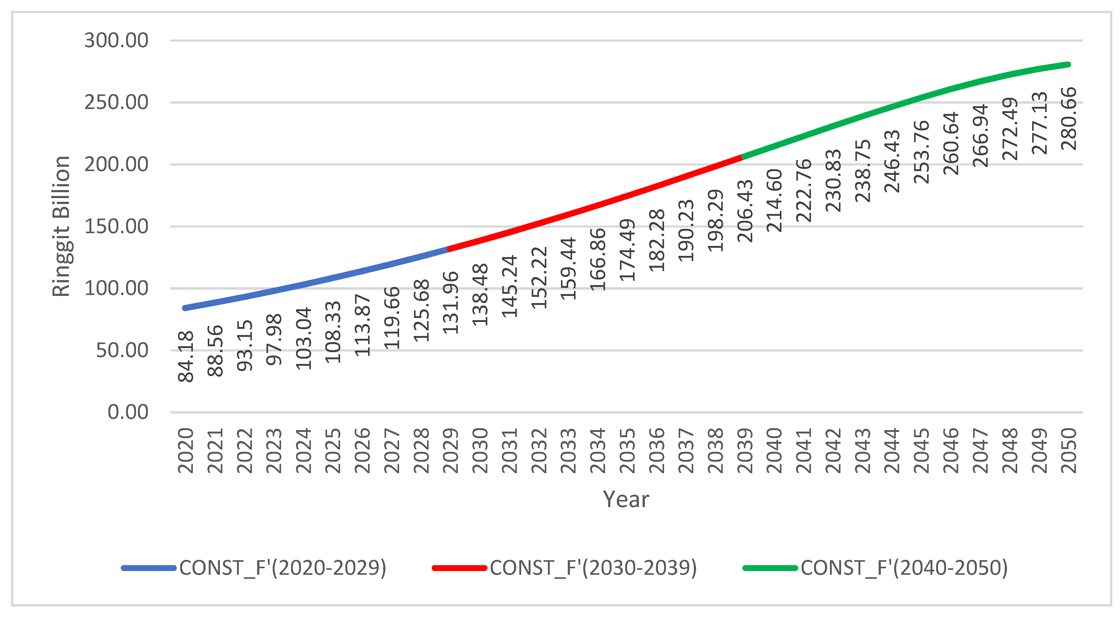
4.13. Predicted Contribution of the Construction Sector to GDP

This study addresses the challenges and the obstacles faced by the MCS to enable competitiveness, self-sufficiency, and effectiveness. The MCS must concentrate on strengthening and upgrading sustainable methods, integrated solutions, timely financing, transparent bidding processes, timely payment and loan releases, resource allocation, ensuring adequate manpower, preference for local skilled workforce than foreign workforce, and R&D to develop innovative methods of construction. These are the factors that hinder the growth of the MCS as compared to neighboring countries.

The government of Malaysia introduced the Shared Prosperity Vision 2030 to provide a decent living standard to all Malaysians by 2030. Under this act, the goal is set to achieve RM 3.4 trillion GDP with a 4.7% increase in annum growth rate within the period of 2021 to 2030. Additionally, this includes increasing the productivity of its major sectors by introducing technology like manufacturing and services by up to 50% and 30%, respectively. The commitment was made to reduce the gap between different income classes, ethnicities, and regions along with the use of the full potential of manpower and resources to optimize the Malaysian economy to its highest potential. It is worth mentioning that developing countries like Malaysia have to face another factor, i.e., the development of the construction sector despite harming the environment [79]. Therefore, a blend of long-term policy and the ethical environmental plan was introduced in Malaysia, commonly referred to as National Transformation Plan 2050 (TN50), under which the country will introduce decisive strategies to cope with household sullage, industrial pollutants, shifting to renewable power sources, and increases in sustainable building practices by 2050. Thus far, the country is heading in the right direction as per TN50 but the effectiveness of this plan can only be assessed in the future [80].

It is evident from the IRF analysis that the Malaysian construction sector is sensitive to shocks in the agriculture and mining sector. That is, a shock in both agriculture and mining sectors will cause a fluctuation in construction sector performance, and the construction sector will take some time before coming back to its position as it was before the shock. In terms of generalization, this study was conducted on Malaysian statistics to assess the behavior of the construction sector in terms of other sectors of the economy, therefore, these results can only be applied to the Malaysian economy as each country has different mechanics of their respective sectors. However, the proposed framework and methodology can be followed in a wider aspect for international sustainable assessment of the construction sector all over the world.

Unlike the study conducted in Australia [45], this work used the IRF to study the behavior of the construction sector and proposed a framework that should be followed to bring the construction sector one step closer to achieving sustainability. When any major contributing sector reaches the maximum capacity of its growth, it can be easily impacted by various factors. This will result in the crash of the nationwide economy, therefore, the government of Malaysia must take into account the results produced by the shock and apply them to the sustainable planning of the sector. This study adds a theoretical contribution towards achieving a sustainable construction sector by studying the effects of short- and long-term initiatives introduced due to the effects of shocks in the construction sector all over the world. The VECM suggests that the construction sector will need both short- and long-term speed adjustments in terms of attaining a sustainable industry when a sustainable policy or greener technology incentives are introduced to the sector. The IRF results indicate that a shock to the construction sector will attract government support for the construction sector, which will incontrovertibly increase the output of the construction sector in the long run and will cause damage to the environment due to increased CO₂ levels unless green technology is made cheaper and affordable. From a global perspective, the VECM results predict that supporting the construction sector will boost the output in the long run, and based on the linkages, it is safe to say that if one sector underperforms, a huge industry like the construction sector will cope with it.

5. Conceptual Framework

The sectorial and sustainable framework consists of three essential steps, namely input, economy-contributing sector, and output. As shown in Figure 7, the input from the government, like budget allocation and resource allocation, is added to the economy-contributing sectors. Each sector has a unique working mechanism in terms of its influence on the country’s economy. Concerning this study, only the construction sector mechanism is shown in detail. This framework suggests that the three inputs in each sector generate their respective outputs. As the scope of this study is the construction sector, it is further broken down into its subcategories. The construction sector is a single industry of collective assistances, namely: stakeholders, productivity measures, and collaborative procurements. These three assistances should be fueled by the latest use of technology, sustainable policies and techniques, and environmentally friendly procedures. Hence, the collaborative support of this framework helps in developing the construction sector. This framework is useful for all the countries that are struggling with embracing sustainability, in particular, in the construction sector. Therefore, the government needs to follow the sustainable construction framework introduced in this study to make the construction industry sustainable and enable this sector to be shockproof from unseen events like a pandemic.

The construction sector depends on stakeholder policies as they define the strategies and actions to improve the prevailing system of construction methods. Productivity measures in the sector ensure that the sector keeps up with the modern needs of the economy. Failure in this innovation and productive plans would lead to underdevelopment and slow projects, which would bring financial strain not only on clients but also on the national funds, therefore, construction method evaluation is necessary over time. The need for collaboration in this sector is of prime interest as it is a huge sector and, without collaborative work, it will collapse. Collapsing and underdevelopment in the construction sector mean less infrastructure, which will reduce the national GDP as the national economy needs adequate infrastructure. The construction sector mechanism revolves around three subcategories, namely administrative policies, technological advancements, and environmental allocation. These three subcategories are interlinked with each other. The administrative policies combined with the modern usage of technology in construction give rise to the sector’s prosperity. Sustainable techniques are employed to give rise to development in the construction sector. The sustainable construction sector in turn ensures social prosperity and its fair share of the national GDP and also avoids environmental degradation, which is possible with resource allocation by the government. This relationship is beneficial from the economical perspective as it clearly states the impact of the construction sector on the economy as well as other sectors. When keeping an eye on the current scenario, it is important to understand how the construction sector contributes to the future. Moreover, this study can be beneficial for other developing countries with similar characteristics to the Malaysian economic sector.

6. Conclusions

Based on the obtained results, it is concluded that the construction sector of Malaysia is connected with other sectors and any direct or indirect change in its input will produce short-term as well as long-term effects on the sector itself and the cumulative GDP. The intersectoral links of SERV, MINI, AGRI, MANU, and CONST are more volatile as compared to the overall GDP, which shows that these sectors are influenced by investors’ trust and other factors apart from the government input. Based on the lowest AIC value of −23.426, the number of lags was selected as two for Granger causality. The linkage direction was assessed based on a p-value less than 0.05. The number of the cointegrating equation was selected as two based on its value of less than 0.05. The selected value of cointegrating and lags was used in the VECM. The VECM with coefficient C(1) = −0.306 and a p-value less than 0.05 indicates the model’s ability to bounce back, which shows the viability of the VECM equation. A DW test value of 2.0 indicated the absence of autocorrelation. The residual and heteroskedasticity with a p-value greater than 0.05 indicate the best forecasting model. Forecasting of the MCS output shows a rise to 131.96 RB, 100 RB, and 80 RB in the years 2020–2029, 2030–2039, and 2040–2050, respectively. The countercyclicality was revealed in this study, which signifies the presence of negative relationships between macroeconomic time series. The results of Granger causality models revealed that the construction sector is greatly influenced by the output of AGRI and SERV sectors and the growth of the CONST sector can be modeled based on the activity in these sectors. The long-term equilibrium of the model established the significance of the construction sector, which shows that overall GDP exhibits a large proportion of the effect on construction sector growth. Hence, this idea supports the fact that the construction industry has the largest contribution to the overall GDP of Malaysia.

The central theme of this study is based on the economic development of all the sectors with fundamental reference to the construction sector and how a change in one sector influences the behavior of other sectors. The empirical results have indicated that all sectors are prone to shocks and might have deteriorating effects on themselves in the short term and on the national economy in the long term. In other words, all sectors must have flexibility and adaptability in case of output shocks in the shortest time possible as failure to perform and generate revenue after the shock might collapse the sector completely, which would result in disastrous effects on the economy. This study has also confirmed the common belief that the construction sector is interdependent on other sectors, illustrating that the construction sector’s behavior will fluctuate with the performance of other sectors in Malaysia.

The outcome of this analysis will be helpful for policymakers, industrialists, stakeholders, and investors, not only in Malaysia but everywhere in the world. Policymakers in Malaysia can understand more about the regulatory measures imposed on the construction sector to determine its role in the national GDP. Similarly, industrialists can determine the effects on the construction sector by examining causal effects in one sector. To protect themselves from atypical circumstances of the economy, like inflation or recession of a country’s economy, investors and stakeholders can make strategies, monetize, and take decisive actions for improving their business which will lead to a sustainable sector. With respect to Malaysia, the joint venture programs between multinational firms and local authorities must be increased to grow sustainability in terms of human capital, increase skilled labor, executing required work in less time, and increasing workers skilled in modern techniques. The sharing of knowledge should be encouraged to increase the trust of local and overseas investors, which will raise foreign direct investments in the construction industry. For wider applicability of the policies, it is recommended that the governments of their respective countries must pay attention to the emphasis of the sustainable construction processes in the sector in terms of legislation, stakeholder trust, human resources, and capacity-building programs.

The VECM has its limitations as the coefficients in it are limited in their ability to forecast the behavior of exogenous and endogenous variables in case of any change in the subsectors of the construction industry, which could give rise to ambiguity in the analysis, therefore, constant updating of the parameters will be required in the VECM. Moreover, any external disruptive shift in technological assets, inflation, and higher market volatility will decrease the forecasting accuracy as the VECM is unable to predict sudden peak changes.

References

1. Musarat, M.A.; Alaloul, W.S.; Liew, M. Impact of inflation rate on construction projects budget: A review. Ain Shams Eng. J. 2020, 12, 407–414. [Google Scholar] [CrossRef]
2. Müller, R.; Veser, M. The current state of nonfinancial reporting in Switzerland and beyond. Die Unternehm. 2020, 74, 296–311. [Google Scholar] [CrossRef]
3. Lean, C.S. Empirical tests to discern linkages between construction and other economic sectors in Singapore. Constr. Manag. Econ. 2001, 19, 355–363. [Google Scholar] [CrossRef]
4. Alaloul, W.; Altaf, M.; Musarat, M.; Javed, M.F.; Mosavi, A. Systematic Review of Life Cycle Assessment and Life Cycle Cost Analysis for Pavement and a Case Study. Sustainability 2021, 13, 4377. [Google Scholar] [CrossRef]
5. Hillebrandt, P.M. Economic Theory and the Construction Industry; Springer: Berlin/Heidelberg, Germany, 1985. [Google Scholar]
6. Alaloul, W.S.; Musarat, M.A.; Liew, M.; Qureshi, A.H.; Maqsoom, A. Investigating the impact of inflation on labour wages in Construction Industry of Malaysia. Ain Shams Eng. J. 2021. [Google Scholar] [CrossRef]
7. Pradip Ajugiya, J.J.B.; Pitroda, J. Comparison of Modern and Conventional Construction Techniques for Next Generation: A Review. In Proceedings of the 21st ISTE State Annual Faculty Convention and National Conference on “Emerging Trends in Engineering”, Tolani Foundation Gandhidham Polytechnic, Adipur, India, 27 December 2016. [Google Scholar]
8. Rafiq, W.; Musarat, M.; Altaf, M.; Napiah, M.; Sutanto, M.; Alaloul, W.; Javed, M.; Mosavi, A. Life Cycle Cost Analysis Comparison of Hot Mix Asphalt and Reclaimed Asphalt Pavement: A Case Study. Sustainability 2021, 13, 4411. [Google Scholar] [CrossRef]
9. Field, B.; Ofori, G. Construction and Economic Development: A Case Study. Third World Plan. Rev. 1988, 10, 41. [Google Scholar] [CrossRef]
10. Gaal, O.H.; Afrah, N. Lack of Infrastructure: The Impact on Economic Development as a case of Benadir region and Hir-shabelle, Somalia. Dev. Ctry. Stud. 2017, 7, 212581063. [Google Scholar]
11. Musarat, M.A.; Alaloul, W.S.; Liew, M.; Maqsoom, A.; Qureshi, A.H. Investigating the impact of inflation on building materials prices in construction industry. J. Build. Eng. 2020, 32, 101485. [Google Scholar] [CrossRef]
12. Khan, R.A. Role of construction sector in economic growth: Empirical evidence from Pakistan economy. In Proceedings of the First International Conference on Construction in Developing Countries (ICCIDC), Karachi, Pakistan, 4–5 August 2008. [Google Scholar]
13. Alaloul, S.W.; Musarat, M.A. Impact of Zero Energy Building: Sustainability Perspective. In Sustainable Sewage Sludge Management and Resource Efficiency; IntechOpen: London, UK, 2020. [Google Scholar]
14. Kenny, C. Construction, Corruption, and Developing Countries; The World Bank: Washington, DC, USA, 2007. [Google Scholar]
15. Estache, A. PPI partnerships vs. PPI divorces in LDCs. Rev. Ind. Organ. 2006, 29, 3–26. [Google Scholar] [CrossRef]
16. Lopes, J.P. Interdependence between the Construction Sector and the National Economy in Developing Countries: A Special Focus on Angola and Mozambique. Ph.D. Thesis, University of Salford, Salford, UK, 1997. [Google Scholar]
17. Geadah, A.N.K. Financing of Construction Investment in Developing Countries Through Capital Markets. Master Thesis, Massachusetts Institute of Technology, Department of Civil and Environmental, Cambridge, MA, USA, 2003. [Google Scholar]
18. Lopes, J. Investment in construction and economic growth. In Economics for the Modern Built Environment; Taylor & Francis: Oxford, UK, 2008; pp. 94–112. [Google Scholar]
19. Rameezdeen, R. Study of Linkages between Construction Sector and Other Sectors of the Sri Lankan Economy. Sri Lanka. 2005. Available online: https://www.iioa.org/conferences/15th/pdf/rameezdeen.pdf (accessed on 2 January 2021).
20. Ofori, G. Construction industry and economic growth in Singapore. Constr. Manag. Econ. 1988, 6, 57–70. [Google Scholar] [CrossRef]
21. Khan, R.A.; Liew, M.S.; Bin Ghazali, Z. Malaysian Construction Sector and Malaysia Vision 2020: Developed Nation Status. Procedia Soc. Behav. Sci. 2014, 109, 507–513. [Google Scholar] [CrossRef] [Green Version]
22. Yu-Chin, C.; Kenneth, R. Are the commodity currencies an exception to the rule? Glob. J. Econ. 2012, 1, 1250004. [Google Scholar] [CrossRef]
23. Cashin, P.; Céspedes, L.F.; Sahay, R. Commodity currencies and the real exchange rate. J. Dev. Econ. 2004, 75, 239–268. [Google Scholar] [CrossRef] [Green Version]
24. Olamade, O.O.; Oyebisi, T.O.; Olabode, S.O. Strategic ICT-use intensity of manufacturing companies in Nigeria. J. Asian Bus. Strategy 2014, 4, 1. [Google Scholar]
25. Drewer, S. Construction and development: A new perspective. Habitat Int. 1980, 5, 395–428. [Google Scholar] [CrossRef]
26. Ofori, G. Challenges of construction industries in developing countries: Lessons from various countries. In Proceedings of the 2nd International Conference on Construction in Developing Countries: Challenges Facing the Construction Industry in Developing Countries, Gaborone, Botswana, 15–17 November 2000. [Google Scholar]
27. Latham, M. Constructing the Team: Final Report of the Government/Industry Review of Procurement and Contractual Arrangements in the UK Construction Industry; Hmso: London, UK, 1994. [Google Scholar]
28. Oladinrin, T.; Ogunsemi, D.; Aje, I. Role of Construction Sector in Economic Growth: Empirical Evidence from Nigeria. Futy J. Environ. 2012, 7, 50–60. [Google Scholar] [CrossRef]
29. Alfan, E.; Zakaria, Z. Review of financial performance and distress: A case of Malaysian construction companies. Br. J. Arts Soc. Sci. 2013, 12, 147. [Google Scholar]
30. Kamar, A.M.; Hamid, Z.A.; Ghani, M.K.; Egbu, C.; Arif, M. Collaboration initiative on green construction and sustainability through Industrialized Buildings Systems (IBS) in the Malaysian construction industry. Int. J. Sustain. Constr. Eng. Technol. 2010, 1, 119–127. [Google Scholar]
31. Hamid, Z.; Kamar, K. Modernising the Malaysian construction industry. In Proceedings of the W089-Special Track 18th CIB World Building Congress, Salford, UK, 10–13 May 2010. [Google Scholar]
32. Malaysia, C. Construction Industry Master Plan Malaysia 2006–2015; Kuala Lumpur; Construction Industry Development Board: Negeri Sembilan, Malaysia, 2007. [Google Scholar]
33. Bin Ibrahim, A.R.; Roy, M.H.; Ahmed, Z.; Imtiaz, G. An investigation of the status of the Malaysian construction industry. Benchmarking Int. J. 2010, 17, 294–308. [Google Scholar] [CrossRef]
34. Kanan, P.D.P.; Bahaman, M.A.T.S. The Key Issues in the Malaysian Construction Industry: Public and Private Sector Engagement; Master Builders Association Malaysia: Kuala Lumpur, Malaysia, 2011. [Google Scholar]
35. Munaaim, C.M.; Dauurl, M.M.; Abdul-Rahman, H. Is late or non-payment a significant problem to Malaysian contractors. J. Des. Built Environ. 2007, 3, 1. [Google Scholar]
36. Department of Statistics Malaysia. Malaysia Economic Performance Fourth Quarter 2020. 2021. Available online: https://www.dosm.gov.my/v1/index.php?r=column/cthemeByCat&cat=100&bul_id=Y1MyV2tPOGNsVUtnRy9SZGdRQS84QT09&menu_id=TE5CRUZCblh4ZTZMODZIbmk2aWRRQT09 (accessed on 2 January 2021).
37. Department of Statistics Malaysia. Malaysia Economic Performance Third Quarter 2020. 2020. Available online: https://www.dosm.gov.my/v1/index.php?r=column/cthemeByCat&cat=100&bul_id=ZlRNZVRDUmNzRFFQQ29lZXJoV0UxQT09&menu_id=TE5CRUZCblh4ZTZMODZIbmk2aWRRQT09 (accessed on 2 January 2021).
38. Department of Statistics Malaysia. Malaysia Economic Performance Third Quarter 2019. 2020. Available online: https://www.dosm.gov.my/v1/index.php?r=column/pdfPrev&id=VDNYYXBkczhkUm9taU9pWUQvSEJBQT09 (accessed on 2 January 2021).
39. Department of Statistics Malaysia. Malaysia Economic Performance Fourth Quarter 2019. 2020. Available online: https://www.dosm.gov.my/v1/index.php?r=column/cthemeByCat&cat=100&bul_id=WWk2MDA3R1k1SlVsTjlzU3FZcjVlUT09&menu_id=TE5CRUZCblh4ZTZMODZIbmk2aWRRQT09 (accessed on 2 January 2021).
40. Hirschmann, R. Value of Construction Work in Malaysia from 2011 to 2019. 2020. Available online: https://www.statista.com/statistics/665028/value-of-construction-work-malaysia/#:~:text=Value%20of%20construction%20work%20in%20Malaysia%202011-2019&text=In%202019%2C%20the%20value%20of,a%20bid%20to%20decrease%20debt (accessed on 2 January 2021).
41. Gamil, Y.; Alhagar, A. The Impact of Pandemic Crisis on the Survival of Construction Industry: A Case of COVID-19. Mediterr. J. Soc. Sci. 2020, 11, 122. [Google Scholar] [CrossRef]
42. Wong, J.M.; Ng, S.T. Forecasting construction tender price index in Hong Kong using vector error correction model. Constr. Manag. Econ. 2010, 28, 1255–1268. [Google Scholar] [CrossRef]
43. Fu, C.; Liu, C. An economic analysis of construction industries producer prices in Australia. Int. J. Econ. Financ. 2010, 2, 3–14. [Google Scholar]
44. Jiang, H.; Xu, Y.; Liu, C. Construction price prediction using vector error correction models. J. Constr. Eng. Manag. 2013, 139, 04013022. [Google Scholar] [CrossRef]
45. Jiang, H.; Liu, C. A panel vector error correction approach to forecasting demand in regional construction markets. Constr. Manag. Econ. 2014, 32, 1205–1221. [Google Scholar] [CrossRef]
46. Shahandashti, S.M.; Ashuri, B. Highway Construction Cost Forecasting Using Vector Error Correction Models. J. Manag. Eng. 2016, 32, 04015040. [Google Scholar] [CrossRef]
47. Faghih, S.A.M.; Kashani, H. Forecasting Construction Material Prices Using Vector Error Correction Model. J. Constr. Eng. Manag. 2018, 144, 04018075. [Google Scholar] [CrossRef]
48. Wong, J.M.; Chan, A.P.; Chiang, Y. Forecasting construction manpower demand: A vector error correction model. Build. Environ. 2007, 42, 3030–3041. [Google Scholar] [CrossRef]
49. Xu, J.-W.; Moon, S. Stochastic forecast of construction cost index using a cointegrated vector autoregression model. J. Manag. Eng. 2013, 29, 10–18. [Google Scholar] [CrossRef]
50. Hyndman, J.R.; Athanasopoulos, G. Forecasting: Principles and Practice; OTexts: Melbourne, Australia, 2018. [Google Scholar]
51. Mak, S.; Choy, L.; Ho, W. Region-specific estimates of the determinants of real estate investment in China. Urban Stud. 2012, 49, 741–755. [Google Scholar] [CrossRef]
52. Hassani, M. Construction Equipment Fuel Consumption During Idling: Characterization Using Multivariate Data Analysis at Volvo CE; Digitala Vetenskapliga Arkivet: Vasteras, Sweden, 2020. [Google Scholar]
53. Zhang, X.; Chen, Y.; Jiang, P.; Liu, L.; Xu, X.; Xu, Y. Sectoral peak CO2 emission measurements and a long-term alternative CO2 mitigation roadmap: A case study of Yunnan, China. J. Clean. Prod. 2020, 247, 119171. [Google Scholar] [CrossRef]
54. Wang, Y.; Wen, Z.; Yao, J.; Dinga, C.D. Multi-objective optimization of synergic energy conservation and CO2 emission reduction in China’s iron and steel industry under uncertainty. Renew. Sustain. Energy Rev. 2020, 134, 110128. [Google Scholar] [CrossRef]
55. Liu, Z.; Ciais, P.; Deng, Z.; Davis, S.J.; Zheng, B.; Wang, Y.; Cui, D.; Zhu, B.; Dou, X.; Ke, P.; et al. Carbon Monitor, a near-real-time daily dataset of global CO2 emission from fossil fuel and cement production. Sci. Data 2020, 7, 1–12. [Google Scholar] [CrossRef] [PubMed]
56. Momade, H.M.; Hainin, M.R. Review of sustainable construction practices in Malaysian construction industry. Int. J. Eng. Technol. 2018, 7, 5018–5021. [Google Scholar]
57. Abidin, N.Z. Sustainable construction in Malaysia–Developers’ awareness. World Acad. Sci. Eng. Technol. 2009, 53, 807–814. [Google Scholar]
58. Musarat, M.; Alaloul, W.; Liew, M.; Maqsoom, A.; Qureshi, A. The Effect of Inflation Rate on CO2 Emission: A Framework for Malaysian Construction Industry. Sustainability 2021, 13, 1562. [Google Scholar] [CrossRef]
59. Hock, I.L.C. Malaysia Needs Sustainable Construction. Malaysia. 2015. Available online: https://www.malaysiakini.com/letters/315928 (accessed on 2 January 2021).
60. Malaysia Department Of Statistics. Available online: https://www.dosm.gov.my/v1/index.php?r=column/cthemeByCat&cat=155&bul_id=aWJZRkJ4UEdKcUZpT2tVT090Snpydz09&menu_id=L0pheU43NWJwRWVSZklWdzQ4TlhUUT09 (accessed on 2 January 2021).
61. Bank, W. Malaysia. 2020. Available online: https://data.worldbank.org/country/MY (accessed on 2 January 2021).
62. Harris, R.I. Testing for unit roots using the augmented Dickey-Fuller test: Some issues relating to the size, power and the lag structure of the test. Econ. Lett. 1992, 38, 381–386. [Google Scholar] [CrossRef]
63. Gujarati, D.N. Basic Econometrics; Tata McGraw-Hill Education: New York, NY, USA, 2009. [Google Scholar]
64. Johansen, S. Statistical analysis of cointegration vectors. J. Econ. Dyn. Control. 1988, 12, 231–254. [Google Scholar] [CrossRef]
65. Johansen, J.S.; Juselius, K. Test. Struct. Hypothesis A Multivar. Cointegration Anal. PPP UIP UK J. Econom. 1992, 53, 1–244. [Google Scholar]
66. Granger, C.W. Investigating causal relations by econometric models and cross-spectral methods. Econom. J. Econom. Soc. 1969, 37, 424–438. [Google Scholar] [CrossRef]
67. Koop, G.; Quinlivan, R. Analysis of Economic Data; Wiley: Chichester, UK, 2000; Volume 2. [Google Scholar]
68. Gujarati, D.N. Basic Econometrics; MacGraw-Hill Inc.: New York, NY, USA, 1995; 838p. [Google Scholar]
69. Granger, C. Some properties of time series data and their use in econometric model specification. J. Econ. 1981, 16, 121–130. [Google Scholar] [CrossRef]
70. Suharsono, A.S. Forecasting Share Price Index In Indonesia and the World with the Univariate and Multivariate Time Series Model. J. Sains Dan Seni Pomits 2013, 2, 2. [Google Scholar]
71. Suharsono, A.; Aziza, A.; Pramesti, W. Comparison of Vector Autoregressive (VAR) and Vector Error Correction Models (VECM) for Index of ASEAN Stock Price. In AIP Conference Proceedings; AIP Publishing LLC: New York, NY, USA, 2017. [Google Scholar]
72. Brown, R.L.; Durbin, J.; Evans, J.M. Techniques for testing the constancy of regression relationships over time. J. R. Stat. Soc. Ser. B Stat. Methodol. 1975, 37, 149–163. [Google Scholar] [CrossRef]
73. Perron, P. The great crash, the oil price shock, and the unit root hypothesis. Econom. J. Econom. Soc. 1989, 57, 1361–1401. [Google Scholar] [CrossRef]
74. Lu, C.; Xin, Z. Impulse-Response Function Analysis: An Application to Macroeconomy Data of China. 2010. Available online: http://www.statistics.du.se/essays/D10_Xinzhou_lucao.pdf (accessed on 2 January 2021).
75. Zikmund, G.W.; Carr, G. Business Research Methods, 7th ed.; Cengage Learning, Dryden: New York, NY, USA, 2000. [Google Scholar]
76. James, H.A. Time Series Analysis; Princton University Press: Princton, NJ, USA; Oxford University: Oxford, UK, 1944. [Google Scholar]
77. Bliemel, F. Theil’s Forecast Accuracy Coefficient: A Clarification; SAGE Publications: Los Angeles, CA, USA, 1973. [Google Scholar]
78. Elengoe, A. COVID-19 outbreak in Malaysia. Osong Public Health Res. Perspect. 2020, 11, 93–100. [Google Scholar] [CrossRef]
79. Government, Malaysia. Shared Prosperity Vision 2030; Percetakan Nasional Malaysia Berhad: Kuala Lumpur, Malaysia, 2019; pp. 1–30.
80. Nielsen, C.; Aalbers, R. Optimal Discount Rates for Investments in Mitigation and Adaptation; CPB Discussion Paper 257; CPB Netherlands Bureau for Economic Policy Analysis: The Hague, The Netherlands, 2013.
Figure 1. Residual correlation of CONST.
Sustainability 13 05012 g001
Figure 2. Structural stability test. (a) CUSUM test. (b) CUSUM square test.
Sustainability 13 05012 g002
Figure 3. Various sector responses. (a) Response of MANU to CONST. (b) Response of CONST to MANU. (c) Response of MINING to CONST. (d) Response of CONST to MINING. (e) Response of AGRI to CONST. (f) Response of CONST to AGRI. (g) Response of SERVC to CONST. (h) Response of CONST to SERVC. (i) Response of GDP to CONST. (j) Response of CONST to GDP. (k) Response of CONST to its shock.
Sustainability 13 05012 g003aSustainability 13 05012 g003b
Figure 4. Fitted forecasted line.
Sustainability 13 05012 g004
Figure 5. Fitted forecasted line for the years 2020–2050.
Sustainability 13 05012 g005
Figure 6. Graphical representation of original and forecasted values 2020–2050.
Sustainability 13 05012 g006
Figure 7. The construction sector and sustainable development as a conceptual framework.
Sustainability 13 05012 g007