The Impact of High-Speed Railway on China’s Regional Economic Growth Based on the Perspective of Regional Heterogeneity of Quality of Place

Abstract

Transport enables trade between people, which is essential for the development of civilizations. Transport is a crucial necessity for specialization, allowing production and consumption of products to occur at different locations. High-speed rail (HSR) allows the flow of people between regions, cities, countries. With rapid global development in HSR technology for passenger transportation, it plays a vital role in transportation systems. The improvement of the quality of cities with different emphasis will bring different economic development results. Therefore, exploring the impact of high-speed railways and quality of place on economic development is necessary. This paper takes the prefecture-level city with a high-speed railway opened in 2008–2013 as the research sample and takes other prefecture-level cities in the country as the control group. The study findings revealed that employment, investment in fixed assets, average wage, and higher education institute significantly affect China’s regional economic growth. Institute of higher education reflects the negative effect on the regional economic growth whereas the employment, investment in fixed assets, and average wage rate positively impact it. Based on the results, it can be concluded that China’s regional economy is significantly affected by its quality.

1. Introduction

Transportation promotes trade between people, which is vital to the development of civilization. Transportation is an essential requirement for specialization so that the production and consumption of products can occur in different locations. Transportation improvements are often considered a precursor to economic growth. In 2016, approximately 35,000 km of the high-speed line ran across the whole world, and more than 2000 km line is to be added [1]. Since the late 1990s, China has been dedicated to building high-speed railways. The introduction of high-speed trains may be the most critical development in passenger transportation in China in the past few decades. The first high-speed rail system, Tokaidu Shinkansen, began operations in Japan in 1964 and is widely known as the bullet train. China’s high-speed rail (HSR) consists of a passenger-dedicated railway network, the most extended high-speed railway network globally, and the most widely used network.

HSR is regarded as the next wave of economic growth [2]. The development of high-speed railways has dramatically improved the connectivity between regions and promoted the flow of factors between regions. With the rapid development of global passenger high-speed rail technology, it plays an essential role in the transportation system [3,4]. As of the third quarter of 2020, China’s domestic high-speed railway network has reached 36,000 km, surpassing the entire network of high-speed railway operations in other countries in the world. According to the mid-to-long-term railway network plan issued by the State Council in 2008 (Figure 1), China will build a “four vertical and four horizontal” railway network by 2020. As the high-speed rail can carry many passengers and shorten the travel time, it has developed as one of the main apparatuses to reduce the traffic burden on Japan, France, Germany, Spain, and recently in some significant transportation corridors in South Korea, Japan, and Taiwan [5].

The massive development of high-speed rail (Figure 2) may promote major cities’ growth and quality of place. Quality of place has been well-defined “as the physical characteristics of a community, planned, designed, developed and upheld that affect the quality of life of individuals living and working” [6]. Disciplines including public health, psychology, economics, and sociology have developed tools for analyzing the QOL experienced by individuals and groups [7]. These characteristics make the place an ideal, competitive, and economically vibrant place to live. Residents living closest to shopping and social service facilities benefit more than those who are further away [8].

Quality may include aesthetics, economics, social, political, environmental, human health, public safety, and other issues. It reveals the integrity of physical, socio-cultural, perceptual, and visual characteristics of a place [9]. High-speed rail (HSR) is expected to significantly impact Chinese cities [10]. Simultaneously, the improvement of the quality of different key cities may bring about different economic development effects. Place plays an essential role in creative cities’ development by ensuring the necessary conditions for creativity [11,12]. Quality of Place includes infrastructure construction, the flow of talents, foreign direct investment, the degree of perfection of the service organization, changes in land price, and increased connectivity. Urban agglomeration shows different development patterns and stages. An urban agglomeration is a highly developed spatial form of integrated cities. Cities are highly integrated into urban agglomerations, making them sources of the most important global economic development [13]. Transportation infrastructure such as high-speed railways is considered a trigger for specific effects of space dynamics. By way of rapid and large-scale transportation across regions, high-speed rail has improved cities’ accessibility and shortened the space–time distance between cities, greatly enhancing cities’ spatial connections along the route [14].

The significance of this study is to find out more about the high-speed rail of China and its effect on quality of place, urban agglomeration and regional economic development of China. The impact of high-speed railways on China’s regional economic development based on its quality of place as the measuring instrument is still uncertain and debatable. This paper selects the prefecture-level cities in 2008–2013 as the research sample. It proposes to examine the relationship between high-speed railway, quality of place, and regional economic using balanced panel data, propensity score matching, and the difference-in-difference (PSM-DID) method and regression analysis. Based on the above, this paper focuses on the following questions and their solution: How do high-speed railways affect regional development through the quality of place? How do high-speed railways through urban agglomeration affect the regional economy? Verify whether high-speed railway significantly affects regional development—How does it affect that development?

2. Literature Review

2.1. Impact of HSR on Economic Growth

Transportation financing is expected to boost economic productivity and economic growth [15]. Traditionally, people have known that transportation infrastructure improvements can promote economic growth in the region [16]. In the classical location theory, the emphasis is on the role of transportation infrastructure in economic development [17]. High-speed railways have brought market structure effects, labor pool effects, knowledge spillovers, and technological innovation effects to cities along the line [18]. High-speed railways may profoundly change China’s regional economy and people’s production and lifestyles.

The rapid development of high-speed railways has dramatically improved the connectivity between regions and strengthened the economic connection between markets. The rapid development of China’s HSR has shortened people’s travel time, improved travel efficiency, and increased economic and personnel communication between different regions and cities. There is a positive impact of transportation infrastructure on economic growth, trade, resource flow, employment, and other aspects [19]. It seems that transportation promotes economic growth, increases regional trade integration, and improves national income level, which creates a spillover effect. As one of the most crucial transportation infrastructures between cities, the high-speed rail may have a substantial economic impact on the cities along the line and has a specific impact on the economic gap between cities. As efficient transportation infrastructure, high-speed rail (HSR) has affected cities’ economies along the route directly and indirectly and had a considerable impact on cities’ economies [20].

2.2. Impact of HSR on Quality of Place

In Europe, the development of high-speed railways has dramatically reduced travel time between cities and reduced space [21]. In addition to promoting the flow of human resources, natural resources, capital, and technology, high-speed railways will also accelerate the flow of knowledge, information and promote closer economic and personnel links between regions [22]. High-speed railways will significantly reduce passengers’ time on travel and accelerate human resources flow [23]. The implementation of HSR has led to the development of the city around the railway station and is said to promote its economic development; most notably, it has led to the reconstruction of many urban station areas [24]. Cultural amenities, crime, green spaces, and congestion are a few of the factors determining the local quality of place [25]. Disciplines including public health, psychology, economics, and sociology have developed tools for analyzing the QOL experienced by individuals and groups [7]. High-speed railway stations may impact central cities’ economic activities and medium-sized surrounding cities. The economic activities gradually transfer from the central city to the surrounding small cities [26].

More and more studies have examined the potential impact of high-speed rail in China from various aspects, including accessibility [27], regional development [28,29], and the real estate market [30,31]. High-speed rail can significantly improve the accessibility of Chinese cities [27,28]. The time–space effect of the “shrinking continent” of high-speed rail will significantly change economic geography [32], forming a corridor of employment, housing, and innovation, and individuals and businesses will be distributed densely around the site [2]. As an efficient transportation infrastructure, high-speed rail (HSR) has affected cities’ economies along the route directly and indirectly and had a considerable impact on cities’ economies [33].

2.3. Impact of HSR on Urban Agglomeration

The opening of high-speed railways will promote the co-urbanization effect of urban agglomerations and accelerate economic exchanges between urban agglomerations [34]. The development of high-speed railway networks will optimize the effective allocation of resources in space. High-speed railways may improve urban development conditions, enhance the connection between the city and a more comprehensive range of markets, industrial chains and increase the market for companies along the route. High-speed rail can promote the free flow of labor, attract corporate headquarters to gather along the high-speed rail, and promote the simultaneous development of regional economic integration and industrial agglomeration [35]. A detailed literature review on the agglomeration impact of transport investment concluded that public transport improvement could bring considerable external benefits by promoting an agglomeration economy [36].

High-speed rail can influence the real estate market by promoting market integration and urban development. The development of high-speed rail service level has been discussed in more detail and it was concluded that high-speed rail reduces the overall travel time [32]. High-speed rail is an essential carrier for achieving interconnection and promoting comprehensive development at home and abroad. Some researchers have given a broader perspective on transportation’s economic consequences, including the coordination and agglomeration benefits of trade benefits and technology diffusion [37]. Urban agglomeration tends to increase its economic growth [38]. Researchers have also investigated the influence of urban agglomeration on economic growth [39]. Urban agglomeration may increase the country’s economic growth.

2.4. Impact of Quality of Place on Urban Agglomeration

Agglomeration economy benefits enterprises and people close to each other in cities and industrial clusters. Urban economists infer the city’s success from high local wages and growth in the number of people in the region. If a place is performing well, employers may pay more for workers in that area, people may be willing to pay more for entering that place, and more people may move to that area. Urbanization continues to increase across the world; the United Nations reported that by the end of 2018 more than 55% of people lived in cities, and this will increase to 68% by 2050. The utmost driving force of urban agglomerations may be growth. The primary reason for the growth may be population migration toward cities and metropolitan regions, driven by the population expectation of finding attractive living conditions. The development of urbanization is a social process in which cities grow and society becomes more urbanized [14].

Urban places include buildings, streets, spaces and landscapes, various land use, and user communities. The physical and social environment can also impact individuals’ economic behavior, happiness, and collective well-being [40]. The basic notion is that more significant transportation activity and road infrastructure construction promote economic growth, and in turn, economic growth may also stimulate infrastructure improvements [33]. In addition to promoting the flow of human resources, natural resources, capital, and technology, high-speed railways will also accelerate the flow of knowledge, information and promote closer economic and personnel links between regions [22].

3. High-Speed Railway Development for Economic Growth Model and Model Setting

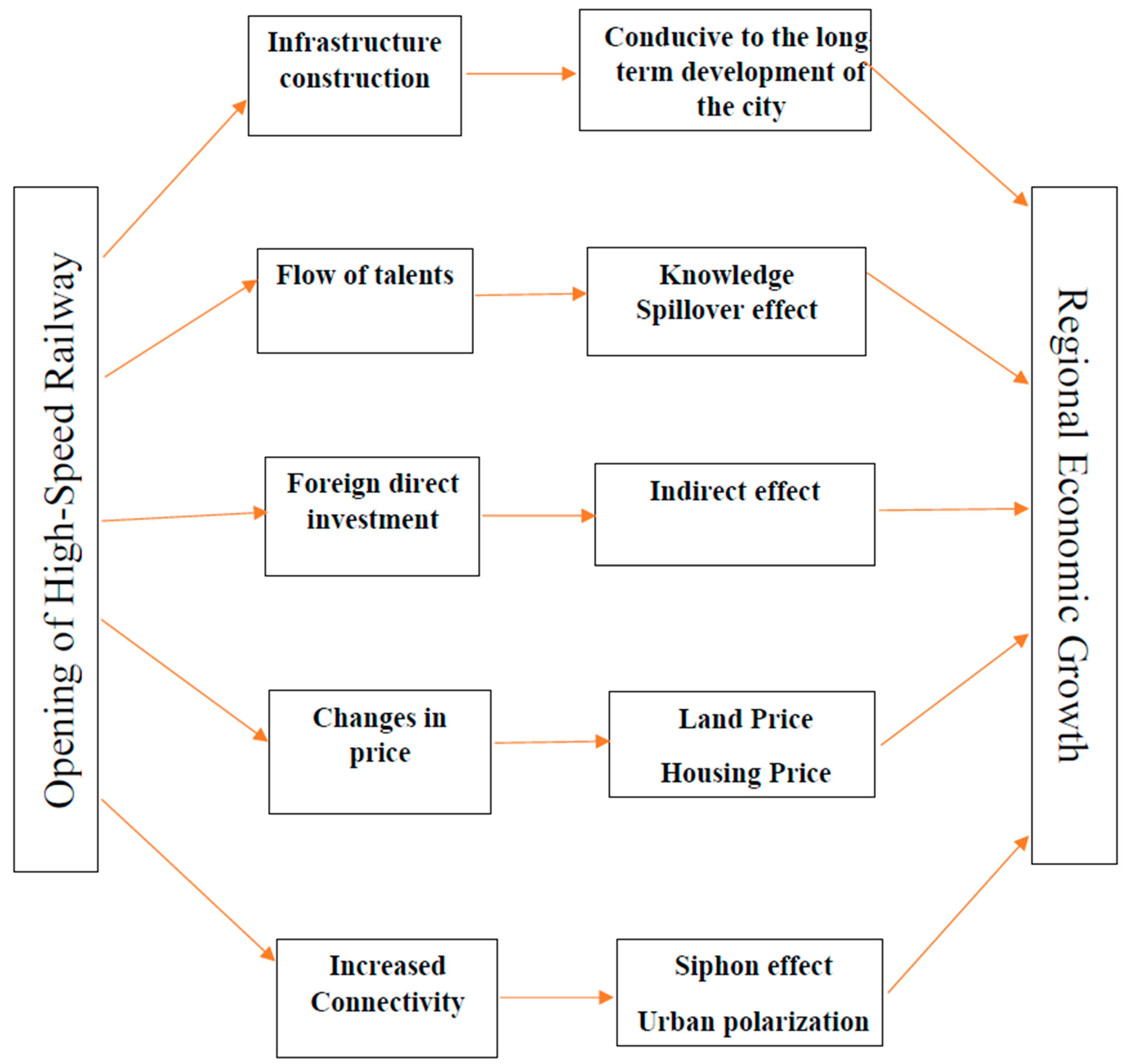
3.1. The Impact Path of High-Speed Railway on the Regional Economic Growth

Various countries have invested in high-speed railway (HSR), where trains are supposed to run. In 2016, it was estimated that approximately 35,000 km of the high-speed line were running across the whole world, and more than 2000 km of line were to be added [1]. There are different motivations of various countries for employing the use of HSR lines. Many countries use HSR lines to facilitate economic growth. It is crucial to identify and measure the economic impact of HSR from different perspectives.

3.1.1. Infrastructure Construction

The Keynesian theory argued that a rise in public spending is aimed at facilitating economic growth [41,42]. HSR plays a significant role in the “subsidy effect” to address the needs of citizens. HSR can support the establishment of relevant infrastructure regarding educational, medical, and educational resources. High-speed rail can reinforce cities’ central business districts and support the growth of businesses and educational institutions. Essential components of human survival, such as transportation, telecommunications, energy, water, sanitation, housing, and educational facilities, are essential for economic activity and social life [43]. Infrastructure is critical to numerous societal sectors: transportation (e.g., roads, railways, ports, and civil aviation); electricity; irrigation; watersheds; hydropower engineering; research, training, and marketing; warehousing; communications and education; and health and family welfare [43]. Infrastructure can also help narrow the regional economic gap, reduce poverty, and improve people’s quality of life and place. In the 1870s, Adam Smith pointed out in Wealth of Nations that good roads, ports, and bridges were necessary conditions for business development and warranted government attention [44].

3.1.2. The Flow of Talents

The travel time improvements from high-speed rail service can also increase productivity by expanding the labor market for businesses looking for talent and increasing opportunities for workers looking for jobs [43]. High-speed rail service helps reduce uneven regional development and encourages the growth of local knowledge industries. The business retention and expansion approach focuses on helping existing firms find new markets for their products, improve their productivity and competitiveness, access a larger labor pool, and attract more customers [43].

While the initial benefit of high-speed rail may be faster travel and increased accessibility, over time it can encourage industries to cluster together and companies to locate in closer proximity to one another in a city’s downtown. This kind of economic agglomeration can lower production costs, concentrate a pool of skilled workers, and stimulate regional economic growth. HSR could have broader economic impacts on cities through its impact on effective employment density, that is, by bringing places of residence and employment closer together by a reduction in travel times [43].

3.1.3. Foreign Direct Investment

Foreign direct investment is usually viewed as a channel for technology to spread from developed countries to developing countries [45,46]. A foreign direct investment (FDI) is an investment made by a firm or individual in one country in business interests located in another country. Generally, FDI occurs when an investor establishes foreign business operations or acquires foreign business assets in a foreign company. Foreign direct investment has a significant influence on China’s regional economic growth [47]. The research has also shown a significant relationship between FDI and economic growth [48].

3.1.4. Changes in Prices

The “drainage” effect of high-speed railways will increase cities’ land prices with high-speed railway stations by an average of about 7.0% compared to cities without stations, and each additional high-speed railway station will increase the city’s land prices by about 1.3% [49]. Local governments will adopt a “horizontal subsidy” strategy when transferring industrial and non-industrial land. This has caused the construction of high-speed railways to increase the price of residential land and commercial service facilities in cities, but the price of industrial land has dropped. HSR plays a key role in housing prices at the city level. The construction of HSR influences key variables responsible for influencing housing prices. The introduction of HSR leads to a 13.9% increase in city-level housing prices, and the figures for national central cities and regional central cities were 31.7% and 19.6%, and the siphon effect and diffusion effect were also observed [50]. HSR services have an impact on the population dynamics and land price in China [51].

3.1.5. Increased Connectivity

The high-speed railway’s opening improves the connectivity between two places, promotes the connection between the cities along the line, and enlarges the “siphon effect” of central cities on peripheral cities [35]. The agglomeration of these cities has a siphonic effect on peripheral cities, which negatively affects their corporate productivity. From this perspective, opening high-speed railways will aggravate the polarization of development between peripheral cities and central cities, causing capital and human resources to flow to central cities [19]. However, another view argued that HSR transfers economic activities from peripheral cities to core cities, resulting in unbalanced regional economic development and damaging the economy’s sustainability. Research has indicated that HSR construction has short-term effects on connectivity and accessibility. It has been noted that the variations in connectivity due to the establishment of HSR have a positive impact on economic development compared to timesaving.

The above literature review is explained diagrammatically in Figure 3.

3.2. Theoretical Model

Based on [52], this paper constructs a multi-regional spatial economic model that includes “high-speed rail factors.” The model includes the cost of goods traded in multiple regions and the commuting cost of people. The model studies the impact mechanism of high-speed rail construction on industrial agglomeration, quality of place, regional employment, wages, and economic growth. The specific model was constructed as follows.

Assume that the economic system consists of a series of locations n and i, where n refers to the classic consumption area, and i refers to the production area. The economy uses a large representative number of consumers to express that they can move freely between regions and supply a unit of inelastic labor with non-negative effects. The adequate labor supply of each region i depends on the region’s labor level L and transportation technology level (bi + ri), where bi is the transportation technology level when the high-speed rail is not built in the region, and ri is the improved transportation technology level after the high-speed rail is built in the region i. If the high-speed rail is not built in the region i, then ri = 0, where the transportation cost is assumed to have an iceberg cost form. For each laborer living in area i, only the (bi + ri) part of the unit labor force is used for production (here 0 < (bi + ri) < 1), and the remaining part is [1 − (bi + ri)], which is the cost of transportation.

Assuming that the total income of area n is equal to the total expenditure, it has the Cobb–Douglas effect [53]. Consumers use the constant proportion of income μ to buy tradable goods. The consumer effect function comprises a series of consumption index C_n of tradable products and illiquid consumption facilities H_n. Here we learn from the practice of Redding et al. [54] and use real estate parameters instead of H_n. Therefore, the Cobb–Douglas effect function form in the above situation can be written as:

$$U_n=C_n^{\mu }{H}_n^{1-\mu } (0<\mu <1).$$

(1)

The consumer price index C_n of the industrial product is expressed as

$$C_n={[{{\displaystyle \sum }}_{i=N}{M}_i{c}_{ni}^{\frac{\sigma -1}{\sigma }}]}^{\frac{\sigma }{\sigma -1}}.$$

(2)

σ is known as the substitution elasticity between variables, and this paper assumed that there is substitutability in variables and (σ > 1); $c_{ni}$ refers to the consumption quantity of the products in the industry in the production area I at the place of consumption n; $M_i$ further represents the products of industry area I and many modern industry products are consumed in the same proportion as the non-industrial products. It was assumed that all products are affected by icebergs’ cost, which is known as the damage costs of the products. During the transportation process the cost will vary depending on the distance, length, and mode of transportation. Furthermore, to transport one unit of goods to the consumption area of n the actual quantity will be measured through ($d_{ni}-f_{ni}$) to the n area where [($d_{ni}-f_{ni}$) − 1] part is transported. Transportation cost will be calculated as there is a loss of transportation due to damage on the way. Here ($d_{ni}-f_{ni}$) > 1, if there are no high-speed railways in the two regions, $f_{ni}$ = 0, otherwise, $f_{ni}$ > 0 where $d_{ni}$ is the traffic volume in the n and i areas without the construction of high-speed railway. Here $f_{ni}$ is the construction of n and I is areas. Moreover, it was assumed that freight volume decreased due to regional transportation improvement and its efficiency to cut costs. The price of the product delivered to the region n, p_i should be

$$p_{ni}=p_i(d_{ni}-f_{ni}).$$

(3)

Moreover, based on applications of Shephard’s lemma, the equilibrium demand of the products of the industrial region n to the region I is as follows:

$$x_{ni}=p_i^{-\sigma }{\left(d_{ni}-f_{ni}\right)}^{1-\sigma }(\mu v_n{L}_n){\left(P_{cn}\right)}^{\sigma -1}.$$

(4)

It was further assumed that the category of products produced by region I has the same demand and elasticity as that for region n and the consumption quantity is replaced by $c_{ni}$ in Formula (2) with the equilibrium demand $x_{ni}$ on the basis of Formula (4). The industrial product price index $p_{cn}$ is derived from the consumer product index C_n, and the formula is as follows:

$$P_{cn}={\left[{{\displaystyle \sum }}_{i=N}{M}_i{P}_{ni}^{1-\sigma }\right]}^{1/\left(1-\sigma \right)}=\{{{\displaystyle \sum }}_{i=N}{M}_i{{(p_i\left(d_{ni}-f_{ni}\right))}^{1-\sigma }\}}^{1/\left(1-\sigma \right)}.$$

(5)

The formulas above indicate that after the opening of HSR $f_{ni}$ > 0, the industrial products’ price decreased, and the residents living in the area can consume products at a low price. Moreover, low prices further indicate that people living in the area will experience high amounts of income. The paper uses the values of $v_n{L}_n$ to represent the total income, and $v_n$ represents the per capita income of city n. Moreover, a consumption ratio was developed that is as follows:

$$P_{an}=\frac{\left(1-\mu \right)v_n{L}_n}{A_n}.$$

(6)

If one individual wants the labor between the cities to stop, actual incomes are considered and equal to other cities. The workers will stop flowing, and when the market of labor is balanced, it will lead to equality, and it can be measured through the following formula:

$$V_n=\frac{v_n}{{\left(P_{cn}\right)}^{\mu }{\left(P_{an}\right)}^{1-\mu }}=V.$$

(7)

As per the assumptions above, the net regional income is equivalent to the net expenditures with the Cobb–Douglas effect, and every region n has a fixed ratio of the industrial product consumption. Hence, for urban n, the net regional income at equilibrium is the labor income and consumption of the non-industrial product composition. At this point, ω_n is used for indicating a level of wage at the consumption area m, and total regional income at the equilibrium point is comprised of labor income and consumption of the non-industrial products.

$$v_n{L}_n={\omega }_n(b_n+r_n)L_n+(1-\mu )v_n{L}_n.$$

(8)

Then the per capital income v_n is reflected as

$$v_n=\frac{{\omega }_n(b_n+r_n)L_n}{\mu }.$$

(9)

The price index shown in Equation (11) is dependent on the category of the industrial product M_i, the offshore price p_i of the production in the i region, and the trade cost of the transportation of the product from region i to region n (d_ni − f_ni), explaining the approachability of the consumer index to the location of the tradable product cma_n is:

$$cm{a}_n\equiv {{\displaystyle \sum }}_{i\in N}{M}_i[p_i{[(d_{ni}-f_{ni})]}^{1-\sigma }.$$

(10)

Hence, the price index P_cn is expressed as

$$P_{cn}={\left[cm{a}_n\right]}^{1/\left(1-\sigma \right)}.$$

(11)

By using the Formulas (5), (6), (9) and (10) to replace P_an, V_n, and P_cn in Equation (11), the condition equation of the labor flow is illustrated as

$$L_n=V^{-1/\left(1-\mu \right)}{\mu }^{-\mu /\left(1-\mu \right)}{\left(b_n+r_n\right)}^{\frac{\mu }{1-\mu }}{A}_{n}H{\omega }_n{}^{\frac{\mu }{1-\mu }}{\left(cm{a}_n\right)}^{\frac{\mu }{\left(1-\mu \right)\left(\sigma -1\right)}}.$$

(12)

In the above equation the level of equilibrium labor L_n is the traffic technology level function (b_n + r_n), the accessibility of the consumer market cma_n, and the real wage ${\omega }_n,$ which is post the HSR completion, the cost of transportation would decline significantly. This will usually enable the producers and consumers to purchase better goods and services from enterprises or regions at a relatively lower prices. The economic activity results transfer will eventually lead to the labor supply transfer as the demand for the work shifts, resulting in labor flow that is derived from the transportation costs. On the other hand, HSR construction will result in changes of the accessibility of the regional market that will encourage enterprises or families to relocate for better production outcomes or a living environment that will lead toward the multiplier effect, resulting in a choice of corporate locations for consumption. The labor equation L_n is generated for the level of the technology traffic (b_n + r_n) that is $\partial L_n/\partial \left(b_n+r_n\right)>0$. The improvement in the level of traffic technology is conducive to the increasing level of labor. The work efficiency per labor unit was assumed to be the same. Hence, the industrial enterprises’ share in the city reflects the percentage of the industrial enterprises’ number in the city:

$$S_C=\frac{L_n}{L}=\frac{V^{-1/\left(1-\mu \right)}{\mu }^{2\mu -1/\mu }{\left(b_n+r_n\right)}^{\frac{\mu }{1-\mu }}{A}_{n}H{\omega }_n{}^{\frac{\mu }{1-\mu }}{\left(cm{a}_n\right)}^{\frac{\mu }{\left(1-\mu \right)\left(\sigma -1\right)}}}{L}.$$

(13)

S_c, L reflect the urban enterprises’ percentage and total labor force in the region in the formula presented above. The S_c is obtained from the technology traffic level (b_n + r_n): since 0 < μ < 1, there is 1 − μ > 0, so $\partial S_C/\partial \left(b_n+r_n\right)$ > 0. The total urban industrial enterprises within the region and transportation technology level are correlated positively. The result is

$$\frac{\partial S_C}{\partial \left(b_n+r_n\right)}=\frac{V^{-1/\left(1-\mu \right)}{\mu }^{2\mu -1/\mu }{\left(b_n+r_n\right)}^{\frac{\mu }{1-\mu }}{A}_{n}H{\omega }_n{}^{\frac{\mu }{1-\mu }}{\left(cm{a}_n\right)}^{\frac{\mu }{\left(1-\mu \right)\left(\sigma -1\right)}}}{\left(1-\mu \right)L}.$$

(14)

Based on this equation, it can be concluded that the HSR results in the improvement of the regional economic growth and can also influence employment. It can further be assumed that the HSR results in a higher level of the quality of place and improves the urban agglomeration by making it more attractive for the public, attracting foreign investments. Hence, the HSR opening would promote the reshaping of employment spaces in the region. Let us suppose city n has opened HSR with r_n > 0. The level of the technology traffic of city n is positively linked with the HSR numbers. In this r_n = ηK_n, η is the correlation coefficient (η > 0) and K_n is the HSR station numbers in n city. By substituting the r_n into the equation and then deriving K_n by the degree of the industrial concentration S_c, the result is represented in Equation (15).

$$\frac{\partial S_C}{\partial K_n}=\eta \frac{V^{-1/\left(1-\mu \right)}{\mu }^{2\mu -1/\mu }{\left(b_n+r_n\right)}^{\frac{\mu }{1-\mu }}{A}_{n}H{\omega }_n{}^{\frac{\mu }{1-\mu }}{\left(cm{a}_n\right)}^{\frac{\mu }{\left(1-\mu \right)\left(\sigma -1\right)}}}{\left(1-\mu \right)L}.$$

(15)

For results derived from Equation (15), it is illustrated that the HSR opening increases the quality of the place, and several of the high-speed railway and industrial enterprise numbers. In combination with the previous conclusion, HSR opening influences the employment, quality of place, and hence this, as a result, increases the city’s regional economic growth.

Hypotheses:

Hypothesis 1 (H1).

HSR has a significant influence on the regional economic growth of China.

As highlighted from the equation above, the HSR influences the regional economic growth of the city. This was further validated by the study of the researcher, which stated that the high-speed railway tends to influence the economic growth of the region significantly [55]. It illustrated that the high-speed railway increases the accessibility and convenience of the place and travel, influencing economic growth. HSR influences China’s regional economic growth, supporting the results [29].

Hypothesis 2 (H2).

Urban agglomeration influences economic growth significantly.

It can also be assumed that urban agglomeration directly influences the economic growth of the region. It can be illustrated that urban agglomeration tends to negatively influence the economic growth of any region since the concentration will lead toward lower growth. Urban agglomeration significantly influences the cities’ economic growth [56]. It was elaborated that urban agglomeration tends to limit the country’s resources, which in turn negatively impacts its economic growth.

Hypothesis 3 (H3).

Foreign direct investment influences the regional economic growth of China.

FDI has also been shown to influence any country’s regional economic growth, and hence it is hypothesized that the FDI influences the regional economic growth of China. It was supported by a research study that found that the FDI has a significant influence on China’s regional economic growth [47].

4. Variables, Data, and Methodology

This section defines variables and describes data. We used prefecture-level data to examine the relationship between HSR development and regional economic growth in China. To measure regional economic growth, we made use of aspects that included quality of place.

4.1. Variables

(a)

Dependent

Gross regional product (GRP) as the dependent variable that depicts China’s economic development. The values were measured per 100 million renminbi.

(b)

Control

Population (Pop) as the proxy for urban agglomeration. The values were measured per 10,000 persons.

• Employment (Emp): The values were measured per 10,000 persons.
• Investment in fixed assets (FA): The values were measured per 10,000 renminbi.
• Foreign direct investment (FDI): The values were measured per unit.
• Investment in the real estate (RE): The values were measured per 10,000 renminbi.
• Park and green areas (P&G): The values were measured by hectares.
• Theaters, music halls and cinemas (TM&C): The values were measured per unit.
• Hospital and health centers (HHC): The values were measured per unit.
• Average wages (AW): The values were measured per renminbi.
• Institute of higher education (IHE): The values were measured per unit.

Table 1. Descriptive Statistics of the main variables.

Variable	Number of Samples	Average Value	Standard Deviation	Minimum Value	Maximum Value
Population	2268	1074.412	621.9086	1	2163
Employment	2268	40.6391	40.6393	0	529.3
Investment in Fixed Asset	2268	1133.501	654.8572	1	2267
Foreign Direct Investment	2268	88.88757	263.0759	0	5096
Investment in Real Estate	2268	1132.359	654.6318	1	2264
Park and Green Area	2268	1073.5	1692.649	0	21165
Theaters, Music Halls and Cinemas	2268	12.59392	16.58828	0	201
Hospital and Health Centers	2268	186.6742	139.6449	1	468
Average Wages	2268	1116.421	653.7362	1	2249
Gross Regional Product	2268	1132.756	654.5287	1	2266
Institute of Higher Education	2268	6.835097	11.65741	0	80

contains number of samples, average value, standard deviation, minimum value and maximum value of all the variables.

4.2. Samples and Data

4.2.1. Sample Selection

This paper drew on the research method of [27], based on the full sample of prefecture-level cities from 2008 to 2013, and selected the city that opened the high-speed railway between 2008 and 2011 as the treatment group, and the remaining samples classified into the control group. This paper’s primary sample data are from prefecture-level cities’ relevant data and above from China City Statistical Yearbook 2007–2013 and China Urban Statistical Bulletin. The final selection was based on 285 cities; the city-wide data were used instead of municipal data, considering the lack of statistical data of some cities or the adjustment of administrative divisions.

4.2.2. Data Acquisition of Prefecture-Level High-Speed Railways

Using the statistical yearbook to collect relevant data, we found that the high-speed railway opening times and transit times at the prefecture-level city level were not available. Therefore, this paper adopted the 2007–2014 paper version of the National Railway Passenger Train Timetable and the software version. Through a manual search (www.12306.cn, accessed on 23 April 2021), the opening times of all prefecture-level cities that have opened high-speed railways (

Table 2. Statistics of prefecture-level cities for high-speed railways opened in 2008–2014.

Year	2008	2009	2010	2011	2012	2013	2014
Newly opened high-speed railway prefecture-level cities	4	9	12	10	28	34	49
Total number of prefecture-level cities	4	13	25	35	63	97	146

) over the years and the high-speed rail transit times between cities were obtained.

4.3. Methodology

Here $GRP$ is gross regional product, $\alpha$ is the constant term, $\beta$ is the parameter for all the control variables. $Emp$ is the employment level, $P\&G$ denotes park and green area, $TM\&C$ is theaters music halls and cinemas. $FDI$ is foreign direct investment, $IHE$ is institute of higher education. $Pop$ is population of the area, $FA$ is the investment in fixed assets. $HHC$ is hospital and health centers, $AW$ is average wages and $RE$ denotes investment in real estate.

$$\begin{array}{c}GRP=\alpha +{\beta }_{1}Emp+{\beta }_{2}P\&G+{\beta }_{3}TM\&C+{\beta }_{4}FDI+{\beta }_{5}IHE+{\beta }_{6}Pop+{\beta }_{7}FA+\\ {\beta }_{8}HHC+{\beta }_{9}AW+{\beta }_{10}RE.\end{array}$$

(16)

Referring to China’s high-speed railway development chronology, we can see that China’s high-speed railway has been in a rapid development period since 2008, so this paper selected 2008 as the starting time for policy implementation. In addition, considering the scope of influence of high-speed railways and their effects on the treatment group cities, this may also impact the control city. Therefore, before using DID, this article referred to the [52] method to remove all cities in the control group and cities in the treatment groups that had not opened high-speed railways to alleviate the possible deviations. This paper drew on the research method of [27] to treat cities with high-speed railways between 2008 and 2011 as treatment groups. To eliminate the negative impacts caused by high-speed policies and accidents, the cities that opened high-speed railways after 2011 were eliminated, and the remaining cities were retained.

The propensity score matching method (PSM) developed by the econometric economists represented can eliminate sample selection bias. Therefore, before doing DID differentiation, selecting a batch of high-speed railway cities with various features and processing groups as similar as possible to the matching group was best. The propensity score matching method can effectively solve sample selection bias, but it cannot avoid the endogeneity problem caused by the variables missing. The double difference rule can solve the endogeneity problem through double difference and get the “policy treatment effect”, but it cannot solve the sample deviation problem well. The two methods complement each other and can more accurately estimate the impact of high-speed rail opening on economic growth. Therefore, this paper used the propensity score matching multiple difference method (PSM-DID).

5. Analysis of Empirical Results

To analyze the data, the researcher utilized three primary techniques. Firstly, the data were analyzed using correlation analysis to determine the linear association, followed by the PSM-DID method and regression analysis. The purpose of the regression analysis was to determine the effect of the independent variables associated with the high-speed railway on China’s regional economic growth. Moreover, to evaluate the robustness of the analysis, multicollinearity and heteroskedasticity were further tested. The results from past studies’ perspectives and the study’s objectives are discussed later.

5.1. Correlation Analysis

Several types of correlation technique were applicable, which comprise Pearson, Kendall, and Spearman’s correlation [57]. The simplest and most straightforward technique to implement was Pearson’s correlation technique. The first and most crucial factor assessed in Pearson’s correlation was the significance of the p-value, which if lower than 0.05 was significant. In the results, the correlation coefficient value that contains the * symbol was determined to have a significant connection. The second factor that was assessed on the Pearson’s correlation was the strength, if the coefficient value of correlation lay between 0 and 1. The value closest to 1 indicated a more robust association, whereas values closer to 0 depicted a weaker association. The strength of variables was categorized on three ranges with respect to the correlation coefficient, where the values ranging from 0.1–0.4 were identified to be a weak association, and coefficients ranging from 0.5–0.7 were determined to have a moderate association.

Table 3. Correlation analysis.

	GRP
Employment	−0.006
Park and Green Area	0.000
Theaters, Music Halls and Cinemas	−0.013
Foreign Direct Investment	0.012
Institute of Higher Education	−0.005
Population	−0.020
Investment in Fixed Assets	0.062 *
Hospitals and Health Centers	−0.001
Average Wages	−0.052 *
Investment in Real Estate	0.138 *

* Significance at 5%.

reflects the correlation analysis results where the association of the GRP was mainly assessed with the factors and mechanisms of high-speed railway and others. The variable GRP was determined to have a significant connection with three variables based on the correlation coefficients with the * symbol. Investment in fixed asset and real estate were determined to positively connect with the GRP of China as the coefficients were 0.062 and 0.138, respectively. Both components were determined to have weak and positive interconnections with the GRP.

On the other hand, the variable average wages had a negative and weak correlation with GRP as the correlation coefficient was computed as −0.052. Hence, as per the correlation technique, the GRP of China was associated with the investment in fixed assets and real estate and the average wages. Other than the discussed variables, the associations of all the remaining variables with GRP were statistically insignificant.

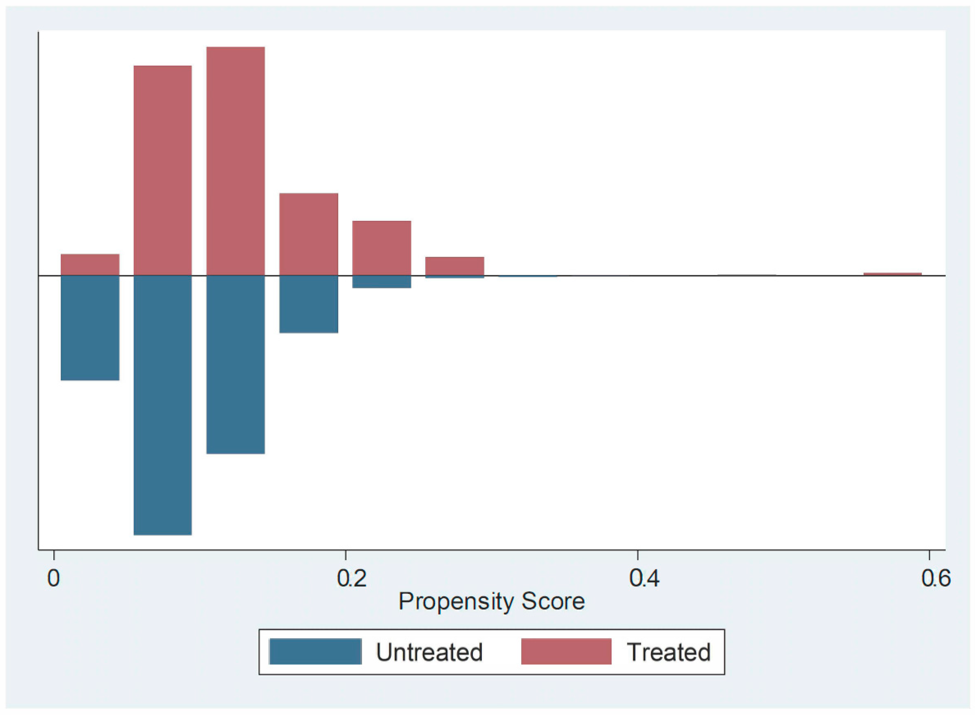
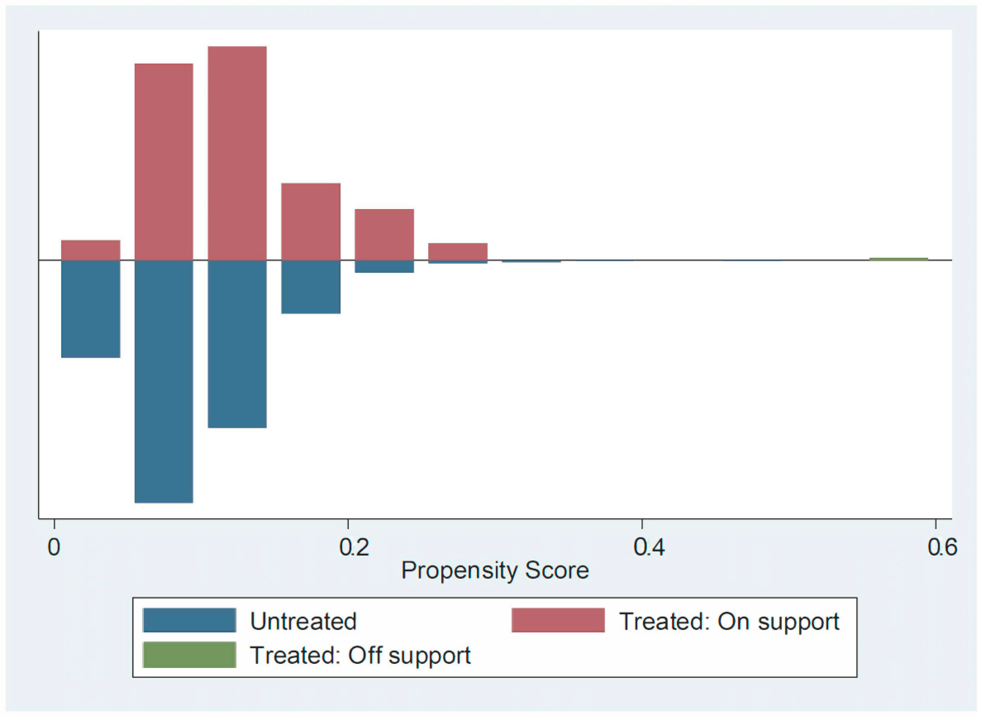
5.2. Propensity Score Matching (PSM)

In order to compare a treated and an untreated group, PSM is one of the most used techniques. The propensity scores matching method (PSM) developed by econometric economists can eliminate sample selection bias. Several reasons contribute to the popularity of propensity score matching; matching can eliminate a more significant portion of bias when estimating the more precise treatment effect than other approaches; matching by the propensity score creates a balanced data set.

In this regard, the results are presented in the

Table 4. PSM model.

	Coef.	Std.	z	p > |z|
LNPOP	−0.140	0.092	−1.520	0.128
Employment	0.003 **	0.002	2.000	0.046
LNIFA	0.271 ***	0.098	2.780	0.006
LNIRE	−0.083	0.058	−1.430	0.153
LNPG	−0.054	0.062	−0.870	0.386
LNHHC	0.076	0.080	0.950	0.344
LNTCM	0.040	0.051	0.790	0.430
LNFDI	−0.047	0.033	−1.410	0.159
LNAW	0.402 **	0.168	2.390	0.017
Institute of Higher Education	−0.009 *	0.005	−1.810	0.070
Constant	−7.763 ***	1.399	−5.550	0.000
LR Chi-Square	55.490		Pseudo R-squared	4.19%
Prob of Chi-square	0.000

***: significant at 1%; **: at 5%; *: at 10%.

. The results indicated that the effect of employment, average wages (LNAW), and investment in fixed assets (LNINFA) are statistically positive and significant on the regional growth (p-value < 0.05). However, the institute’s effect was computed to be statistically significant at 10% (p-value = 0.070 < 0.1). Moreover, overall, the model was also statistically significant while Pseudo r-squared was computed to be 4.19%, meaning that the variance in all the independent variables reflected a 4.19% variance in China’s regional growth.

In terms of evaluating treated vs. untreated groups, the results are presented in

Table 5. PSM testing.

Variable	Sample	Treated	Controls	Difference	S.E.	T-Stat
LNGRP	Unmatched	16.29	15.99	0.30	0.07	4.61
	ATT	16.29	16.28	0.02	0.09	0.16

, where the difference was statistically insignificant.

5.3. PSM-DID and Robustness Model Testing

To determine the treatment effects using a better approach, the researcher used the PSM-DID technique, where interaction effects were computed and added to test in the model. The results in this regard are presented in

Table 6. PSM-DID Model.

	Coef.	Std. Error	t	p > |t|
LNPOP	0.18 ***	0.01	13.11	0.00
Employment	0.00 ***	0.00	14.82	0.00
LNIFA	0.52 ***	0.01	34.89	0.00
LNIRE	0.03 ***	0.01	3.01	0.00
LNPG	0.14 ***	0.01	14.49	0.00
LNHHC	−0.04 ***	0.01	−3.19	0.00
LNTCM	0.06 ***	0.01	7.94	0.00
LNFDI	0.04 ***	0.00	8.79	0.00
LNAW	0.18 ***	0.03	7.18	0.00
Institute of Higher Education	−0.01 ***	0.00	−9.18	0.00
Year*City	−0.01	0.04	−0.35	0.73
City	0.00	(omitted)
Year	0.03	0.03	1.02	0.31
Constant	3.54 ***	0.20	17.63	0.00
F-statistics	1809.47		R-squared	91.44%
Probability of f	0.000		Adjusted R-squared	91.39%

***: significant at 1%; **: at 5%; *: at 10%.

, where the treated group consisted of the cities that built high-speed railway before 2011, whereas the time variable included the period before 2011 as the time group. It was inferred from the table that the effects of population (LNPOP), employment, investment in fixed asset (LNIFA), investment in real estate (LNIRE), park and green areas (LNPG), theaters, music halls and cinemas (LNTCM), foreign direct investment (LNFDI), and average wages (LNAW) were statistically positive and significant. In addition, the effect of hospital and health centers (LNHHC) and institute of higher education were computed to be statistically negative and significant on the regional economic growth. The interaction effect was inconsequential, showing no significant difference between the treatment and control groups. The variance in all the independent variables and the interaction effects explained 91.44% variance in the regional economic growth.

In the following model, robust errors were used where the results were quite similar; however, the variable LNIRE was significant at 10% with robust errors that can be seen in

Table 7. PSM-DID model with robust errors.

	Coef.	Std. Error	t	p > |t|
LNPOP	0.18 ***	0.02	9.09	0.00
Employment	0.00 ***	0.00	6.59	0.00
LNIFA	0.52 ***	0.02	26.48	0.00
LNIRE	0.03 *	0.02	1.90	0.06
LNPG	0.14 ***	0.02	7.63	0.00
LNHHC	−0.04 ***	0.01	−3.11	0.00
LNTCM	0.06 ***	0.01	7.41	0.00
LNFDI	0.04 ***	0.01	7.33	0.00
LNAW	0.18 ***	0.03	5.17	0.00
Institute of Higher Education	−0.01 ***	0.00	−7.84	0.00
Year*City	−0.01	0.03	−0.37	0.71
City	0.00	(omitted)
Year	0.03	0.03	1.08	0.28
Constant	3.54 ***	0.31	11.58	0.00
F-statistics	1687.83		R-squared	91.44%
Probability of f	0.000

***: significant at 1%; **: at 5%; *: at 10%.

.

5.4. Parallel Line Testing

The assumption associated with difference-in-difference (DID) was of parallel line or trend. In this regard, Figure 4 and Figure 5 are presented as follows, and they depict that the assumption was met.

5.5. Heterogeneity Testing and Placebo Testing

In order to determine the heterogeneity, the treated and placebo regions were tested separately, as shown in

Table 8. Heterogeneity testing.

	Coef.	Std. Error	t	p > |t|
LNPOP	0.28 ***	0.09	3.29	0.00
Employment	0.01 ***	0.00	3.53	0.00
LNIFA	0.43 ***	0.07	6.26	0.00
LNIRE	0.11 *	0.05	2.00	0.05
LNPG	0.04	0.04	1.07	0.29
LNHHC	−0.01	0.06	−0.12	0.90
LNTCM	0.01	0.04	0.36	0.72
LNFDI	0.05 *	0.02	1.99	0.05
LNAW	0.55 ***	0.19	2.95	0.00
Institute of Higher Education	−0.01 ***	0.00	−4.06	0.00
Constant	0.11	1.40	0.08	0.94
F-statistics	206.84		R-squared	93.83%
Probability of f	0.000

***: significant at 1%; **: at 5%; *: at 10%.

and

Table 9. Placebo group.

	Coef.	Std. Error	t	p > |t|
LNPOP	0.18 ***	0.02	8.79	0.00
Employment	0.00 ***	0.00	6.53	0.00
LNIFA	0.52 ***	0.02	26.39	0.00
LNIRE	0.03 *	0.02	1.68	0.09
LNPG	0.14 ***	0.02	7.81	0.00
LNHHC	−0.04 ***	0.01	−3.20	0.00
LNTCM	0.06 ***	0.01	7.53	0.00
LNFDI	0.04 ***	0.01	7.10	0.00
LNAW	0.18 ***	0.04	5.14	0.00
Institute of Higher Education	−0.01 ***	0.00	−7.64	0.00
Constant	3.56 ***	0.31	11.62	0.00
F-statistics	1900.39		R-squared	91.41%
Probability of f	0.000

***: significant at 1%; **: at 5%; *: at 10%.

, respectively. The results associated with the treatment group indicated that the effects of LNPOP, employment, LNIFA, LNIRE, LNAW were statistically positive and significant. The effect of the institute of higher education was statistically significant yet negative. Overall, the model was significant, and the variance explained was 93.93%.

In the placebo group, all variables were statistically significant and defined the regional growth of China appropriately. However, the effect of LNHHC and the institute of higher education were statistically negative. Also, the model was statistically significant, while the variance explanation was 91.41%. This can be seen in Table 9.

5.6. Equilibrium Testing

In order to determine the equilibrium, the differences between the groups were evaluated. The results in

Table 10. Equilibrium testing.

Outcome Var		LNGRP	Standard Error	t-Statistics	Probability
Before
	Control	3.538
	Treated	3.525
	Diff (T-C)	−0.013	0.037	−0.35	0.727
After
	Control	3.565
	Treated	3.552
	Diff (T-C)	−0.013	0.037	0.35	0.727
Diff-in-Diff		0.00
R-square:	91%

indicated that even before treatment and after treatment, the difference between the treated and control groups was statistically insignificant (p-value > 0.05). Therefore, no effect of treatment over the period was found in China’s case and its regional economic growth associated with the high-speed railway. The variance explained was computed to be 91%.

5.7. Ordinary Least Square Regression (OLS)

The regression analysis was mainly conducted for testing the linear dependency of one or more variables on the dependent variable. The dependent variable of the study was the gross domestic product, which reflected the economic development of the regions in China. Other than that, the independent variables were taken in according to the theoretical model. The result of the OLS is provided in

Table 11. OLS regression.

GRP	Coef.	Std. Err.	t	p > |t|
Employment	0.162	0.633	0.260	0.798
Park and Green Area	0.004	0.014	0.280	0.783
Theaters, Music Halls and Cinemas	−0.421	0.915	−0.460	0.645
Foreign Direct Investment	0.042	0.068	0.620	0.538
Institute of Higher Education	0.150	1.776	0.080	0.933
Population	−0.024	0.024	−1.020	0.309
Investment in Fixed Assets	0.049 **	0.021	2.310	0.021
Hospitals and Health Centers	−0.002	0.098	−0.020	0.983
Average Wages	−0.064 ***	0.022	−2.870	0.004
Investment in Real Estate	0.131 ***	0.021	6.220	0.000
Constant	1016.535	51.580	19.710	0.000
F (10,2257)	5.85		R-squared	2.53%
Probability of F	0.000

***: Significant at 1%; **: at 5%; *: at 10%.

. With respect to the model, it was statistically significant as the p-value of the f-statistics was calculated as 0.00, which was below the 0.05 threshold.

Moreover, the independent variable variance that depicted the high-speed railway was predicted by 2.53% among the variance of the regional economic growth. While analyzing the individual variables, it was determined that the effect of investment in fixed assets was statistically significant on China’s regional economic growth while the effect was positive (B = 0.049; p-value = 0.021 < 0.05). Furthermore, the effect of average wages was computed to be statistically negative yet significant (B = −0.064; p-value = 0.004 < 0.01). Lastly, the effect of investment in real estate was computed to be statistically positive and significant (B = 0.131; p-value = 0.00 < 0.01). Other than the discussed variables, the effect of all the remaining variables was statistically insignificant.

5.8. Multicollinearity Testing

For the determination of issues in the residuals and data, the researcher conducted diagnostic testing. Therefore, to evaluate the presence of multicollinearity in the data, the researcher utilized the variance inflation factor (VIF). Some researchers have defined multicollinearity as an issue where the variables are positively correlated, producing spurious regression results [58]. Following these studies the maximum acceptable level of the VIF was 10; however, values above 6 were also considered as highly collinear [59]. Therefore, the results in this regard are presented in

Table 12. Multicollinearity testing.

Variable	VIF	1/VIF
Employment	3.57	0.28
Park and Green Area	2.99	0.33
Institute of Higher Education	2.32	0.43
Foreign Direct Investment	1.71	0.58
Theaters, Music Halls and Cinemas	1.24	0.80
Population	1.17	0.86
Average Wages	1.15	0.87
Investment in Fixed Assets	1.05	0.96
Investment in Real Estate	1.03	0.98
Hospital and Health Centers	1.01	0.99
Mean VIF	1.72

. The results indicated that none of the variables positively correlated with the other variable, since the individual VIFs were below 5, whereas the VIF was also below 5.

5.9. Heteroskedasticity Testing

Heteroskedasticity is referred to as the issue in the residual of the regression models, usually where variances across the data set are not constant [60]. In this regard, the researcher tested ordinary least squares (OLS) regression, and the results were tested for heteroskedasticity. Therefore, the Breusch–Pagan/Cook–Weisberg test was applied, whose null hypothesis stated that the variances were constant or homoscedastic. The results are presented in

Table 13. Heteroskedasticity testing.

Breusch–Pagan/Cook–Weisberg Test for Heteroskedasticity
Chi-square	73.83
Probability Value	0.00

. In this regard, the results showed that the OLS model’s residuals were heteroskedastic since the p-value was 0.000 < 0.05 with a chi-square of 73.83. Consequently, the results must be fixed, and the OLS model cannot be deemed robust.

5.10. Robust Regression Analysis

Regression is referred to as a statistical test where the linear dependency of one or more variables is tested on another variable that is known as the dependent or exploratory variable [61]. In this regard, the following study used gross regional product (GRP) as the dependent variable depicting China’s economic development. The independent variables were taken in accordance with the proposed model. The results are presented in

Table 14. Robust regression analysis.

Variables	Coef.	Std. Error	T	p > |t|
Employment	0.162	0.666	0.240	0.808
Park and Green Area	0.004	0.012	0.310	0.758
Theaters, Music Halls and Cinemas	−0.421	0.825	−0.510	0.610
Foreign Direct Investment	0.042	0.052	0.800	0.425
Institute of Higher Education	0.150	1.734	0.090	0.931
Population	−0.024	0.024	−1.010	0.312
Investment in Fixed Assets	0.049 **	0.022	2.180	0.029
Hospitals and Health Centers	−0.002	0.096	−0.020	0.983
Average Wages	−0.064 ***	0.022	−2.900	0.004
Investment in Real Estate	0.131 ***	0.023	5.660	0.000
Constant	1016.535 ***	46.678	21.780	0.000
F (10,2257)	5.120		R-squared	2.53%
Probability of F	0.000

***: significant at 1%; **: at 5%; *: at 10%.

, where robust standard errors were used since there was an issue of heteroskedasticity that was discussed earlier.

The overall model was found to be statistically significant based on the p-value of the f-statistics, which was computed to be 0.00 < 0.05. On the other hand, the variance in all the independent variables depicting high speed was found to explain 2.53% of the variance in the regional economic growth. Individually, it was found that the effect of investment in fixed assets was statistically significant on the regional economic growth of China while the effect was positive (B = 0.049; p-value < 0.05). This indicated that with the improvement in fixed assets investment, the regional economic growth will also improve. Moreover, the effect of average wages was computed to be statistically negative yet significant (B = −0.064; p-value < 0.01). Contrarily, the effect of investment in real assets was computed to be statistically positive and significant (B = 0.131; p-value < 0.01). Other than the discussed variables, the effect of all the remaining variables was statistically insignificant.

5.11. Discussion

5.11.1. HSR Has a Significant Influence on Regional Economic Growth

The study was conducted to identify the effect of HSR on the economic growth of the city. Many studies have been conducted previously on identifying the influence of HSR on economic growth. Some studies have identified the influence that high-speed railway (HSR) networks have on economic growth [62]. The empirical analysis of the study identified that the HSR launch tends to influence economic growth significantly. Researchers have also investigated the influence of the HSR on economic growth, and it was identified that large cities tend to have a significant influence that increases economic growth significantly [35]. The findings of this study are supported by a study that also found that the opening of the HSR tends to impact economic growth significantly, and, in this way, the study findings are strongly supported [22]. Researchers have further enhanced studies on the impact of HSR on economic development [63]. This study evaluated the HSR impact on sustainable economic development and found that they are significantly related to each other.

5.11.2. HSR Along with Quality of Place Improves Regional Economic Growth

The study was further conducted to identify the influence of HSR and the quality of place. It was evaluated in the previous studies that the HSR tends to improve the quality of the place and economic growth. HSR tends to influence the different aspects of a city, and it improves the quality of the city in different aspects [1]. This study found that the HSR opening also influences the quality of place. HSR development will reduce the distance between the cities and consequently produce higher accessibility and transportation convenience, which will increase market structure, the labor pool, and innovation transfer of the cities. High-speed railways tend to increase the quality of place since it is perceived that it increases accessibility and convenience of traveling [51]. The significant relationships between the quality of place and HSR were revealed in this study, consistent with previous studies’ findings.

5.11.3. HSR Along with Urban Agglomeration Improves the Regional Economic Growth of China

The influence of HSR development was also identified in this study, and it was demonstrated that HSR tends to have a significant effect on China’s regional economic growth and urban agglomeration. The population was considered as the proxy for the urban agglomeration, and it was found that HSR development tends to have a significant link with the population. HSR tends to play an essential role in urban agglomeration [38]. The study indicated that HSR construction tends to increase the average network density of urban agglomeration, which positively promotes urban agglomeration’s spatial connection density. It was also identified that HSR can improve the centrality point of the cities that are moderately developed and reduce the urban agglomeration dependence on central cities, as well as improve the stability of urban agglomeration of the spatial structure.

High-speed railway (HSR) has a positive and significant impact on urban agglomeration [51]. This indicates that the HSR tends to influence the urban agglomeration to influence the spatial capability. The studies support this study’s findings and are consistent with the previous studies and findings; it is revealed that HSR can have a significant influence on urban agglomeration.

5.11.4. Urban Agglomeration has a Significant Influence on Economic Growth

The research also evaluated the impact of the quality of place on urban agglomeration, and it identified that urban agglomeration was not found to have a significant influence on economic development. However, previous studies have found a significant influence of urban agglomeration on economic development. Urban agglomeration tends to increase economic growth [38]. They have also investigated the influence of urban agglomeration on economic growth [39]. It was identified that urban agglomeration tends to increase the country’s economic growth, and, hence, HSR leading to higher urban agglomeration can also lead toward economic growth. Urban agglomeration tends to influence economic growth positively and significantly [64]. The finding of this study was not consistent with the findings of the previous studies.

6. Conclusions and Policy Recommendations

6.1. Conclusions

Transportation is vital for the development of the country and civilization. Therefore, countries have been emphasizing improving their transportation infrastructure to promote the region’s economic growth. Since 1990, China has been committed to developing high-speed railways, where it has introduced high-speed trains in the field of passenger transportation over the past few decades. This research aimed to determine whether China’s high-speed railway leads to regional economic development. Several kinds of research have been conducted, but the less developed areas in China remain controversial. Hence, the following research was mainly conducted to investigate the effect of high-speed railways on regional development based on urban industrial agglomeration quality.

The results revealed that the factors contributing to economic growth are investments in real estate and in fixed assets, whereas the average wage was determined to negatively influence China’s economic growth. Therefore, based on the results, it can be concluded that the high-speed railway in China is mainly enhanced by investing in the fixed assets that can lead toward the improvement of the infrastructure and thus contribute to economic growth. Moreover, it was determined that the high-speed train, along with real estate investment, leads to China’s regional economic growth.

6.2. Policy Recommendation

As per the results, a few policies are recommended for China that not only support improving its high-speed railway but also contribute toward the regional economic growth, which are the following:

• It is recommended that the government enhance the promotion of the human and natural resources and the capital and technology of HSR that would help accelerate the knowledge and information flow. The employment and wage rate must be improved for achieving more refined regional economic growth. It is also recommended to increase the economic growth by more investment in the fixed assets.
• The government of China can strengthen its policies related to the development of the infrastructure of HSR that can improve transportation services.
• It is recommended that China improve its real estate industry by reconstructing most of the urban station areas, which can increase the reliability of the high-speed railways and further boost China’s economic growth.
• It is further recommended to focus on the aspects of higher education institutions that would negatively impact the economic growth of the region.
• Further, it is recommended that more employment opportunities are implemented.

6.3. Future Implication of the Research

The study’s future implication is that the researchers can employ the subjective view, based on interviews with the authorities, which can help them gain detailed information regarding the importance of the high-speed railway to China’s economic growth. Furthermore, a similar method can be incorporated in other developing countries such as Russia, Brazil, or India to understand the importance of high-speed railway.

References

1. Bharule, S.; Kidokoro, T.; Seta, F. Evolution of High-Speed Rail and Its Development Effects: Stylized Facts and Review of Relationships; ADBI Working Paper 1040; Asian Development Bank Institute: Tokyo, Japan, 2019. [Google Scholar]
2. Tierney, S. High-speed rail the knowledge economy and the next growth wave. J. Transp. Geogr. 2012, 22, 285–287. [Google Scholar] [CrossRef]
3. Bonnafous, A. The Regional Impact of the TGV. Transportation 1987, 14, 127–137. [Google Scholar] [CrossRef]
4. Givoni, M. Development and Impact of the Modern High-speed Train: A Review. J. Transp. Rev. 2006, 26, 593–611. [Google Scholar] [CrossRef]
5. Cheng, Y.H. High-speed rail in Taiwan: New experience and issues for future development. Transp. Policy 2010, 17, 51–63. [Google Scholar] [CrossRef]
6. Department for Communities and Local Government. Community, Opportunity, Prosperity; Annual Report; Communities and Local Government: London, UK, 2009. [Google Scholar]
7. Raphael, D.; Renwick, R.; Brown, I.; Rootman, I. Quality of life indicators and health: Current status and emerging conceptions. Soc. Indic. Res. 1996, 39, 65–88. [Google Scholar] [CrossRef]
8. Vaz, E.; Venter, C.J. The Effectiveness of Bus Rapid Transit as Part of a Poverty-Reduction Strategy: Some Early Impacts in Johannesburg. In Proceedings of the 31st Southern African Transport Conference, Pretoria, South Africa, 9–12 July 2012. [Google Scholar]
9. Durmaz, S.B. Analyzing the Quality of Place: Creative Clusters in Soho and Beyoğlu. J. Urban Des. 2014, 20, 93–124. [Google Scholar] [CrossRef]
10. Yin, M.; Bertolini, L.; Duan, J. The Effects of the High-Speed Railway on Urban Development: International Experience and Potential Implications for China. Prog. Plan. 2015, 98, 1–52. [Google Scholar] [CrossRef] [Green Version]
11. Florida, R. The Rise of the Creative Class: And How It’s Transforming Work, Leisure, Community and Everyday Life; Basic Books: New York, NY, USA, 2002; 404p. [Google Scholar]
12. Trip, J.J. What Makes a City: Urban Quality in Euralille, Amsterdam South Axis and Rotterdam Central; OTB Research Institute for Housing, Urban and Mobility Studies, Delft University of Technology: Delft, The Netherlands, 2008; pp. 79–99. [Google Scholar]
13. Fang, C.; Zhou, C.; Gu, C.; Chen, L.; Li, S. A proposal for the theoretical analysis of the interactive coupled effects between urbanization and the eco-environment in mega-urban agglomerations. J. Geogr. Sci. 2017, 27, 1431–1449. [Google Scholar] [CrossRef]
14. Wang, F.; Wei, X.; Liu, J.; He, L.; Gao, M. Impact of high-speed rail on population mobility and urbanization: A case study on Yangtze River Delta urban agglomeration, China. Transp. Res. Part A 2019, 127, 99–114. [Google Scholar]
15. Aschauer, D.A. Is public expenditure productive? J. Monet. Econ. 1989, 23, 177–200. [Google Scholar] [CrossRef]
16. Chandra, S.; Vadali, S. Evaluating accessibility impacts of the proposed America 2050 high-speed rail corridor for the Appalachian Region. J. Transp. Geogr. 2014, 37, 28–46. [Google Scholar] [CrossRef]
17. Weber, A. Industrial Location Theory. 1997. Available online: economia.unam.mx/cedrus/descargas/Libro%20de%20Weber.pdf (accessed on 23 April 2021).
18. Aldieri, L.; Vinci, C.P. Firm Size and Sustainable Innovation: A Theoretical and Empirical Analysis. Sustainability 2019, 11, 2775. [Google Scholar] [CrossRef] [Green Version]
19. Yang, X.; Lin, S.; Li, Y.; He, M. Can high-speed rail reduce environmental pollution? Evidence from China. J. Clean. Prod. 2019, 239, 118135. [Google Scholar] [CrossRef]
20. Li, X.; Wu, Z.; Zhao, X. Economic effect and its disparity of high-speed rail in China: A study of mechanism based on synthesis control method. Transp. Policy 2020, 99, 262–274. [Google Scholar] [CrossRef]
21. Spiekermann, K.; Wegener, M. The shrinking continent: New time-space maps of Europe. Environ. Plan. B Plan. Des. 1994, 21, 653–673. [Google Scholar] [CrossRef]
22. Zhang, X.L. Does China’s Transportation Infrastructure Promote Regional Economic Growth? Concurrently on the Spatial Spillover Effect of Transportation Infrastructure. Chin. Soc. Sci. 2012, 3, 60–77. [Google Scholar]
23. Delaplace, M.; Pagliara, F.; Perrin, J.; Mermet, S. Can High Speed Rail foster the choice of destination for tourism purpose? Procedia Soc. Behav. Sci. 2014, 111, 166–175. [Google Scholar] [CrossRef] [Green Version]
24. Trip, J.J. What Makes a City? Planning for Quality of Place. Sustainable Urban Areas Development; IOS Press: Amsterdam, The Netherlans, 2007. [Google Scholar]
25. Andrews, C.J. Analyzing quality-of-place. Environ. Plan. B Plan. Des. 2001, 28, 201–217. [Google Scholar] [CrossRef] [Green Version]
26. Shao, S.; Tian, Z.; Yang, L. High speed rail and urban service industry agglomeration: Evidence from China’s Yangtze River Delta Region. J. Transp. Geogr. 2017, 64, 174–183. [Google Scholar] [CrossRef]
27. Shaw, S.L.; Fang, Z.; Lu, S.; Tao, R. Impacts of high-speed rail on railroad network accessibility in China. J. Transp. Geogr. 2014, 40, 112–122. [Google Scholar] [CrossRef]
28. Zhu, Y.; Diao, M. The impacts of urban mass rapid transit lines on the density and mobility of high-income households: A case study of Singapore. Transp. Policy 2016, 51, 70–80. [Google Scholar] [CrossRef]
29. Chen, Z.; Haynes, K.E. Impact of high-speed rail on regional economic disparity in China. J. Transp. Geogr. 2017, 65, 80–91. [Google Scholar] [CrossRef]
30. Zheng, S.; Matthew, E. Kahn China’s bullet trains facilitate market integration and mitigate the cost of megacity growth. Proc. Natl. Acad. Sci. USA 2013, 110, E1248–E1253. [Google Scholar]
31. Diao, X.; Harttgen, K.; McMillan, M. The Changing Structure of Africa’s Economies. World Bank Econ. Rev. 2017, 31, 412–433. [Google Scholar] [CrossRef] [Green Version]
32. Vickerman, R. Location, accessibility, and regional development: The appraisal of trans-European networks. Transp. Policy 1995, 2, 225–234. [Google Scholar] [CrossRef] [Green Version]
33. Li, H.; Liu, Y.; Peng, K. Characterizing the relationship between road infrastructure and local economy using structural equation modeling. Transp. Policy 2018, 61, 17–25. [Google Scholar] [CrossRef]
34. Zhang, Q.; Nie, X. High-Speed Rail Construction and the Regional Economic Integration in China. Mod. Urban Res. 2010, 6, 7–10. [Google Scholar]
35. Li, F.; Su, Y.; Xie, J.; Zhu, W.; Wang, Y. The Impact of High-Speed Rail Opening on City Economics along the Silk Road Economic Belt. Sustainability 2020, 12, 3176. [Google Scholar] [CrossRef] [Green Version]
36. Chatman, D.G.; Noland, R.B. Do Public Transport Improvements Increase Agglomeration Economies? A Review of Literature and an Agenda for Research. Transp. Rev. 2011, 31, 725–742. [Google Scholar]
37. Lakshmanan, T.R. The broader economic consequences of transport infrastructure investments. J. Transp. Geogr. 2011, 19, 1–12. [Google Scholar] [CrossRef]
38. Zhang, P.; Zhao, Y.; Zhu, X.; Cai, Z.; Xu, J.; Shi, S. Spatial structure of urban agglomeration under the impact of high-speed railway construction: Based on the social network analysis. Sustain. Cities Soc. 2020, 62, 102404. [Google Scholar] [CrossRef]
39. Khan, H.U.; Awan, M.A. Possible factors affecting internet addiction: A case study of higher education students of Qatar. Int. J. Bus. Inf. Syst. 2017, 26, 261–276. [Google Scholar]
40. Royuela, V.; Moreno, R.; Vayá, E. Is the influence of quality of life on urban growth non-stationary in space? A case study of Barcelona. IREA Work. Pap. 2007, 3, 200703. [Google Scholar]
41. Lee, J.C.; Won, Y.J.; Jei, S.Y. Study of the Relationship between Government Expenditures and Economic Growth for China and Korea. Sustainability 2019, 11, 6344. [Google Scholar] [CrossRef] [Green Version]
42. Keynes, J.M. The General Theory of Money, Interest and Employment. In The CollectedWritings of John Maynard Keynes; Palgrave Macmillan: London, UK, 1936; p. 7. [Google Scholar]
43. Harnessing High-Speed Rail: How California and Its Cities Can Use Rail to Reshape Their Growth; SPUR (San Francisco Bay Area Planning and Urban Research Association): San Francisco, CA, USA, 2017.
44. Hutchison, T. Adam Smith and The Wealth of Nations. J. Law Econ. 1976, 19, 507–528. [Google Scholar] [CrossRef]
45. Balasubramanyam, V.N.; Salisu, M.; Sapsford, D. Foreign Direct Investment and Growth in EP and IS Countries. Econ. J. 1996, 106, 92–105. [Google Scholar] [CrossRef]
46. Borenztein, E.; De Gregorio, J.; Lee, J.W. How does foreign direct investment affect economic growth. J. Int. Econ. 1998, 45, 115–135. [Google Scholar] [CrossRef] [Green Version]
47. Sothan, S. Causality between foreign direct investment and economic growth for Cambodia. Cogent Econ. Financ. 2017, 5, 1277860. [Google Scholar] [CrossRef]
48. Islam, M.A.; Khan, M.A.; Popp, J.; Sroka, W.; Oláh, J. Financial Development and Foreign Direct Investment—The Moderating Role of Quality Institutions. Sustainability 2020, 12, 3556. [Google Scholar] [CrossRef]
49. Zhou, Y.; Yang, J.; Huang, Y.; Geoffrey, J.D.H. Research on the impact of high-speed rail on urban land prices and its mechanism: Evidence from microscopic land transactions. China Ind. Econ. 2018, 5, 118–136. [Google Scholar]
50. Wang, Y.; Liu, X.; Wang, F. Economic Impact of the High-Speed Railway on Housing Prices in China. Sustainability 2018, 10, 4799. [Google Scholar] [CrossRef] [Green Version]
51. Rungskunroch, P.; Yang, Y.; Kaewunruen, S. Does High-Speed Rail Influence Urban Dynamics and Land Pricing? Sustainability 2020, 12, 3012. [Google Scholar] [CrossRef] [Green Version]
52. Dong, Y.; Zhu, Y. Can high-speed rail construction reshape China’s economic, spatial layout based on the regional heterogeneity perspective of employment, wages, and economic growth? China Ind. Econ. 2016, 10, 92–108. [Google Scholar]
53. Cobb, C.W.; Douglas, P.H. A Theory of Production (PDF). Am. Econ. Rev. 1928, 18, 139–165. [Google Scholar]
54. Redding, S.J.; Weinstein, D.E. Measuring Aggregate Price Indexes with Taste Shocks: Theory and Evidence for CES Preferences; NBER: Cambridge, UK, 2016. [Google Scholar]
55. Yao, S.; Zhang, F.; Wang, F.; Ou, J. Regional economic growth and the role of high-speed rail in China. Appl. Econ. 2019, 51, 3465–3479. [Google Scholar] [CrossRef]
56. Giersch, H. Urban Agglomeration and Economic Growth; Springer: Berlin, Heidelberg, 1995. [Google Scholar]
57. Tkachenko, I.; Destruel, C.; Strauss, O.; Puech, W. Sensitivity of different correlation measures to print-and-scan process. Electron. Imaging 2017, 7, 121–127. [Google Scholar] [CrossRef] [Green Version]
58. Silvestrini, R.T.; Burke, S.E. Linear Regression Analysis with JMP and R; Quality Press: Seattle, WA, USA, 2018. [Google Scholar]
59. Moy, R.L.; Chen, L.S.; Kao, L.J. Study Guide for Statistics for Business and Financial Economics: A Supplement to the Textbook by Cheng-Few Lee, John C. Lee and Alice C. Lee; Springer: Berlin, Germany, 2014. [Google Scholar]
60. Lee, C.F.; Chen, H.Y.; Lee, J. Financial Econometrics, Mathematics and Statistics; Springer: New York, NY, USA, 2019. [Google Scholar]
61. Kleinbaum, D.G.; Kupper, L.L.; Nizam, A.; Rosenberg, E.S. Applied Regression Analysis and other Multivariable Methods; Nelson Education, Cengage Learning: Boston, MA, USA, 2013. [Google Scholar]
62. Zou, W.; Chen, L.; Xiong, J. High-Speed Railway, Market Access, and Economic Growth; ADBI Working Paper 852; Asian Development Bank Institute: Tokyo, Japan, 2018. [Google Scholar]
63. Guo, B.; Ke, J. The Impacts of High-speed Rail on Sustainable Economic Development: Evidence from the Central Part of China. Sustainability 2020, 12, 2410. [Google Scholar] [CrossRef] [Green Version]
64. Jayasooriya, S.P. Urban agglomeration and regional economic growth in China. Empir. Econ. Rev. 2019, 33, 281–295. [Google Scholar]
Figure 1. Growth of China’s high-speed rail network in the year 2008 (https://elibrary.worldbank.org/doi/pdf/10.1596/978-1-4648-1425-9, accessed on 23 April 2021).
Sustainability 13 04820 g001
Figure 2. Growth of China’s high-speed rail network in the year 2018 (https://elibrary.worldbank.org/doi/pdf/10.1596/978-1-4648-1425-9, accessed on 23 April 2021).
Sustainability 13 04820 g002
Figure 3. Pathway of the impact of high-speed railways on the regional economic growth. (Source: Author).
Sustainability 13 04820 g003
Figure 4. Parallel line testing.
Sustainability 13 04820 g004
Figure 5. Parallel line testing with treated group.
Sustainability 13 04820 g005