Cyclic Weighted k-means Method with Application to Time-of-Day Interval Partition

Abstract

Time-of-day interval partition (TIP) at a signalized intersection is of great importance in traffic control. There are two shortcomings of the traditional clustering algorithms based on traditional distance definitions (such as Euclidean distance) of traffic flows. First, some continuous time intervals are usually divided into small segments. Second, 0 o’clock (24 o’clock) is usually selected as the breakpoint. It follows that the relationship between TIP and traffic signal control is neglected. To this end, a novel cyclic distance of traffic flows is defined, which can make the end of the last cycle (24 o’clock of the last day) and the beginning of the current cycle (0 o’clock of the current day) cluster into one group. Next, a cyclic weighted k-means method is proposed, with centroid initialization, cluster number selection, and breakpoint adjustment. Lastly, the proposed method is applied to a real intersection to evaluate the benefits of traffic signal control. The conclusion of the empirical study confirms the feasibility and effectiveness of the method.

1. Introduction

In an urban road network, the traffic signal control at intersections has a great impact on traffic flow. A reasonable traffic signal control scheme can improve the efficiency of traffic flow and relieve traffic congestion. On the contrary, traffic congestion will be worse if an inappropriate scheme is implemented.

Traffic signal control can be divided into three categories according to the range of control: isolated intersection control, arterial coordination control [1,2], and area coordination control [3,4]. Among them, isolated intersection control is the most universally applied. Most schemes of isolated intersection control are fixed-time control mode. First, it can make efficient use of historical data in urban transportation networks [5] and behave well no matter whether under low-medium saturation degree [6] or certain oversaturated conditions [7,8,9,10]. Second, it is a substitute when the malfunction of detectors or data loss occurs. Furthermore, it can behave as a kind of supplement in those intersections without traffic flow detectors.

There are two main tasks for fixed-time control mode. One is called the time-of-day interval partition (TIP) problem that traffic managers usually need to divide the whole day into different time intervals, e.g., peak hours, off-peak hours, etc. The other is the determination of signal control scheme for each time interval. An appropriate TIP plan is the precondition for the optimization of traffic signal control schemes at the isolated intersection [11]. Moreover, a reasonable traffic signal control scheme is able to improve the efficiency of traffic flow operations and relieve traffic congestion.

In recent decades, a large proportion of researches takes TIP as a clustering problem, determining the optimal breakpoints of time intervals [12,13]. Clustering is an unsupervised learning technique which can discover potential structures of data. It is also an important tool for exploratory data analysis, especially when the volume of data is quite large. Clustering algorithms are aimed at automatically classifying data points into groups based on their similarity and distribution. In the field of machine learning, distance-based clustering (or similarity-based) is the most popular paradigm for clustering, including k-means, k-medoids, hierarchical clustering, and spectral clustering [14]. In the field of statistics, model-based clustering attracts more attention, such as the EM algorithm of a Gaussian mixture model [15,16,17]. However, no matter what kinds of methods are used, a common problem is to determine the number of clusters. Most clustering methods require a given number of clusters. However, in recent years, clustering methods that do not require the number of classes in advance have been developed, such as affinity propagation [18], density peaks-based clustering [19], time-variant clustering [20], and robust continuous clustering [21]. These methods can automatically output the number of clusters as well as the cluster assignments.

In the existing literature, inspired by [22], k-means clustering is the prevailing method of TIP, and some refinements, such as pretreatment or transformation of data, are step-wisely added to the basic k-means clustering framework [23,24,25,26,27,28]. However, the main problem of k-means is that the sampling units with similar traffic flows are more easily assigned into one cluster, ignoring the continuity of time. It means some noncontinuous sampling units could be assigned into one cluster. For example, two sampling units 7:00–7:05 and 17:00–17:50 should not be clustered together even though their traffic flows are similar. In other words, the partition results of traffic volumes are not continuous in time, so manual adjustment is necessary. If the traffic flow changes dramatically, the partition results may be unsatisfactory due to the subjective and lagging adjustment. From this point of view, TIP should take both the continuity of time and the similarity of traffic flows into account to meet the complex traffic situations.

Some researchers have noted that the order of the partition result matters. Many sequential clustering methods, such as times series partitioning [29], genetic algorithm [30,31,32], Kohonen neural network [33], artificial immune clustering [34], etc., are applied in TIP, and have been successfully employed in the daily scheme of traffic systems. One drawback in these studies is that 0 o’clock (24 o’clock) must be set as a breakpoint of daily data in clustering algorithms, which is unreasonable in practice. Moreover, the distance measurements used in these algorithms, such as Euclidean distance [26,27,29,33,34] in each cycle (each day), are also inappropriate to some degree. According to the definition of Euclidean distance, the distance between 0 and 24 o’clock is the largest among all time points. In fact, 0 and 24 o’clock are identical, and the distance between them should be 0. As a result, these methods cannot connect the end point of the previous cycle and the start point of the current cycle in their clustering results. For example, 23:55 and 0:05 could not be assigned into the same cluster. This does not meet the principles of traffic flow. Since there are few vehicles at 23:55 and 0:05, they both belong to low-peak hour. For this purpose, the cyclic property of flow data should be considered when using clustering algorithms in TIP.

In fact, none of the foregoing methods can be directly applied to the clustering of cyclic data due to the following two reasons. (1) In different cycles, the division of intervals should be the same; (2) Usually, the critical point of two adjacent cycles should be clustered into one interval unless the critical point is a jump point. According to these two requirements, a novel clustering algorithm based on cyclic distance is proposed, called the cyclic weighted k-means method.

In practical applications, it is difficult to obtain the exact moment of vehicles passing through an intersection. Instead, one can only roughly count the traffic flow in each sampling unit. Therefore, the middle point of each sampling unit is taken as the representative time point, while the traffic flow in the sampling unit is regarded as the frequency of traffic transit (i.e., the weight of the traffic transit moment). Then, the TIP problem could be effectively solved based on such data.

In this study, a type of flow data is defined as cyclic data, which is collected from N cycles in succession with T sampling units in each cycle. Next, a cyclic weighted k-means clustering method is proposed for this type of data. This method provides a new idea for directly programming timeline of time intervals with multiple cycles of data via defining a cyclic distance between any two time points. In this method, the traffic flow is used as weights for time points. Similar to k-means clustering, the proposed method is sensitive to the initial values. To this end, an initialization method of centroids was developed, considering the practical traffic background.

In addition, for the sake of evaluation, some existing criteria can be used [35], but the relationship between TIP and traffic signal control is hard to express. In the traffic engineering field, the purpose of TIP is to serve the traffic signal control. More specifically, TIP influences vehicle delays, cycle length, split and offset [7,10,36], queue length [37], saturation degree [1], intersection capacity, etc. Furthermore, TIP also influences urban transportation network design [38], vehicle routing [39,40], bus scheduling [41,42], freight-transportation systems [43] in the practical applications. Thus, TIP is the prerequisite for traffic signal control, which directly improves the effect of traffic control and affects implicitly urban transportation planning. Accordingly, a cost function is adopted according to specific urban traffic problems, and one evaluation criterion is calculated on the partition results of the proposed clustering method [30].

The rest of this article is organized as follows. Section 2 describes the problem of this study. Next, Section 3 introduces the cyclic distance and the cyclic weighted k-means method with some details. In addition, the outstanding performance of the proposed method is numerically confirmed on an empirical dataset of traffic flows in Section 4. Lastly, some concluding remarks are given in Section 5.

2. Problem Description

The TIP problem of traffic signal control is to optimally determine the breakpoint along the timeline of one day, then an optimal signal timing plan for each time interval will be set according to the results of TIP. Traditional methods to solve this problem are to sample the traffic flow of one or more lanes in a $w$ minute (usually 5 min) sampling unit at a traffic intersection. Then, we get the traffic flows (i.e., the numbers of vehicles passing a lane at a traffic intersection) of $T$ sampling units per day (usually $T=288$) and use some kinds of clustering algorithms to divide time intervals. However, the result of TIP based on only one-day traffic flow data are not robust. In order to make up for this, the traffic flow data are collected for several days in order to improve the stability of TIP. In the rest of the article, one day is called one cycle because the change in daily traffic flows with time is similar.

In this study, the traffic flow data were collected in a signalized traffic intersection for $N$ consecutive days (also called $N$ cycles), taking $w$ minutes as a sampling unit. Let $X=\left(x_1,\dots ,x_N\right) ЄR^{T\times N}$ be a $N$-cycle traffic flow matrix where T is the number of sampling units in one cycle, $x_n={\left(x_{1n},\dots ,x_{Tn}\right)}^{\prime }$ is the traffic flow vector on the n-th ($1\le n\le N$) cycle with T units, $x_{tn}$ is the traffic flow of the t-th ($1\le t\le T$) sampling unit on the n-th cycle. Note that the summation of the t-th row of $X$ (i.e., ${\displaystyle \sum }_{n=1}^N{x}_{tn}$) is the total traffic flow of the t-th sampling unit over $N$ cycles, and the summation of n-th column of $X$ (i.e., ${\displaystyle \sum }_{t=1}^T{x}_{tn}$) is the total traffic flow of the n-th day. Further, let ${\rm B}={\left(B_1,\dots ,B_T\right)}^{\prime }$ be a timescale vector where $B_t=\left(t-1\right) w/1440$ is the start point of the t-th sampling unit in one cycle because there are 1440 min per day. Obviously, the timescale vector ${\rm B}$ is an ordered measure of cyclic data $X$, satisfying $0=B_1<B_2<\dots <B_T<1$.

According to the above definitions, the TIP problem can be described as finding K breakpoints $0\le A_1<\dots <A_K<1$ based on cyclic data $X$ and timescale ${\rm B}$. Then, one cycle can be divided into $K$ time intervals $D_1,D_2,\dots ,D_K$ where $D_k=\left[A_k,A_{k+1}\right)$ for $1\le k\le K-1$ and $D_K=\left[0,A_1\left]{{\displaystyle \cup }}^{}\right[A_K,1\right)$. Note that the time interval $D_K$ crosses 0 o’clock. Driven by this formulation of the TIP problem, the cyclic weighted k-means algorithm will be derived, and the optimal breakpoints $A_1,\dots ,A_K$ will be obtained based on cyclic data $X$ and timescale ${\rm B}$ in the following section.

3. Methodology

3.1. Cyclic Distance

The definition of distance will greatly affect the results of distance-based clustering algorithms (such as k-means). For the TIP problem, 0 and 24 o’clock refer to the same time, which means that the distance between them should be 0. In order to make the end of the last cycle (i.e., 24 o’clock of the last day) and the beginning of the current cycle (i.e., 0 o’clock of the current day) cluster into one group, a cyclic distance is defined between any two different timescales $B_i$ and $B_j$ as

$$d\left(B_i,B_j\right)=\left[\min (\left|B_i-B_j\left|,1-\right|B_i-B_j\right|\right){]}^2$$

(1)

The cyclic distance describes the cyclic characteristic of data on the interval $\left[0,1\right)$, which treats 0 and 1 as the same point. If the Euclidean distance of timescales $B_i$ and $B_j$ is not greater than 0.5 in one cycle (i.e., one day), then their cyclic distance is the squared Euclidean distance. Otherwise, if the Euclidean distance of timescales $B_i$ and $B_j$ is greater than 0.5 in one cycle, then the cyclic distance of them can be viewed as the squared Euclidean distance in two adjacent cycles. In other words, if one point is close to 0 and another point is close to 1, then they should be close in the sense of cyclic distance.

3.2. Cyclic Weighted k-means Method

The classical k-means clustering algorithm can be redefined according to the definition of cyclic distance. In this subsection, the cyclic weighted k-means algorithm will be derived based on cyclic traffic flow data $X$ and timescale $B$. The objective is to segment $B_1,\dots ,B_T$ into $K$ (i.e., the cluster number) time intervals $D_1,\dots ,D_K$ by breakpoints $A_1,\dots ,A_K$. The objective function of the cyclic weighted k-means algorithmcan be represented as

$$J\left(K\right)={\displaystyle \sum }_{k=1}^K{\displaystyle \sum }_{B_t\in D_k}{y}_{t}d\left(B_t,{\mu }_k\right)$$

(2)

In Equation (2), $y_t={\displaystyle \sum }_{n=1}^N{x}_{tn}$ is the total traffic flow of the t-th sampling unit over N cycles, centroid ${\mu }_k$ is the weighted mean of timescales in the k-th time interval $D_k$ with traffic flows as the weights, which can be calculated by

$${\tilde{\mu }}_k={\displaystyle \sum }_{B_t\in D_k}{y}_t{B}_t/{\displaystyle \sum }_{B_t\in D_k}{y}_t$$

(3)

$${\mu }_k={\tilde{\mu }}_k-I\left({\tilde{\mu }}_k\ge 1\right)+I({\tilde{\mu }}_k<0)$$

(4)

where $I(\bullet )$ is the indicator function that is equal to 1 if the condition in the parentheses is satisfied and equal to 0 otherwise. Equation (4) can ensure that the centroid ${\mu }_k$ lies in the interval $\left[0,1\right]$, and avoid falling on the right side of 1 or the left side of 0.

The cyclic weighted k-means algorithm solves the minimum of objective function (2) by iterative steps. It can find the $K$ centroids minimizing the cyclic distances within clusters (also called intra-class distance); that is, the summation of the cyclic distance from each data point to its own centroid. Then, the breakpoints of time intervals are determined. Since the objective function (2) is non-convex, the solution obtained by the iterative steps is often locally optimal.

The cyclic weighted k-means algorithm is given in Algorithm 1.

Algorithm 1. The cyclic weighted k-means algorithm
Require: iterations $I=100$, number of sampling units $T$, cluster number $K$.
Ensure: Determine the centroids ${\mu }_1^i,\dots ,{\mu }_K^i$ and breakpoints $A_1,\dots ,A_K$ in i-th iteration.
1:	Initialize the iterative number $i=0$ and centroids ${\mu }_k^i$ (see Algorithm 2).
2:	for$i\leftarrow 1$ to $I$ do
3:	for$t\leftarrow 1$ to $T$ do
4:	Class label of t-th timescale $B_t$ in i-th iteration $c_t^i={\mathrm{argmin}}_k\left\{d\left(B_t,{\mu }_k^i\right)\right\}$ where $c_t^i\in \left\{1,\dots ,K\right\}$, i.e., assign a centroid to timescale $B_t$ in i-th iteration.
5:	End for
6:	for$k\leftarrow 1$ to $K$ do
7:	Update the centroids: ${\mu }_k^{i+1}={\displaystyle \sum }_{c_t^i=k}{y}_t[B_t+I(\left|B_t-{\mu }_k^i\right|>0.5)\left(-1{)}^{I({\mu }_k^i<0.5)}\right]/{\displaystyle \sum }_{c_t^i=k}{y}_t$.
8:	End for
9:	If${\displaystyle \sum }_{k=1}^K\left|{\mu }_k^{i+1}-{\mu }_k^i\right|\ne 0$then
10:	Output centroids ${\mu }_1^i,\dots ,{\mu }_K^i$ and class labels $c_1^i,\dots ,c_T^i$.
11:	Obtain $K$ subscripts $t_1,t_2,\dots ,t_K$ which satisfy $c_t^i\ne c_{t-1}^i$ (let $c_0^i=c_T^i$, $1\le t\le T$).
12:	Obtain the corresponding $K$ breakpoints $B_{t_1},B_{t_2},\dots ,B_{t_K}$.
13:	Ranking from small to large, the final breakpoints $A_1,\dots ,A_K$ are obtained.
14:	Break
15:	End if
16:	End for

Remark 1.

In line 4, we can see that the algorithm determines the centroids of $B_t$s according to the distance in time domain. Obviously, the timescales divided by the algorithm must be continuous.

Remark 2.

In line 7, the weighted mean of all $B_t$s in k-th cluster is calculated with traffic flow as the weights to update the centroids. Note that, the second item in square bracket is to ensure that the updated centroids lie on the interval $\left[0,1\right]$.

Remark 3.

If the medoids instead of centroids are updated in Step 3, it is converted into the cyclic weighted k-medoids algorithm. As one can see, the minimum of objective function $\tilde{J}\left(S\right)={\displaystyle \sum }_{t=1}^T{\displaystyle \sum }_{c_t\in S}{y}_{t}d\left(B_t,B_{c_t}\right)$ can be obtained approximately by iteration, and the class labels of data points are accordingly obtained where $S\subset \left\{1,\dots ,T\right\}$ is the set of class labels. The cardinality of S (i.e., $K=\left|S\right|$) is the number of clusters. $c_t$ is the class label of the t-th timescale; that is, $B_t$ belongs to the cluster with medoid $B_{c_t}$. Note that, the cyclic weighted k-medoids algorithm will not be introduced here because it is similar to the cyclic weighted k-means algorithm in thinking.

3.3. Initialization of Centroids

The result of TIP will affect the traffic control scheme. Theoretically speaking, the time interval of traffic signal control can be very short. However, in practice, the setting of traffic lights cannot be switched too frequently. Thus, the initial values of centroids should be selected appropriately. In other words, the initial values of centroids should not be too crowded in Algorithm 1. Otherwise, it could cause some time intervals to be too short to operate in reality. On the other side, setting appropriate initial values of centroids will further improve the efficiency of the clustering algorithm. In this subsection, a novel initialization method of centroids for cyclic weighted k-means algorithm will be developed.

Let $y_{max}$ be the local maximum of sequence $y_1, \dots ,y_T$, and the corresponding timescale be $B_{max}$. For a fixed $K$, there exists some function $\delta \left(K\right)>0$, then the cyclic $\delta \left(K\right)$ neighborhood of $B_{max}$ is defined as

$$U\left(B_{max},\delta \left(K\right)\right)=\left\{B_t|\sqrt{d\left(B_t,B_{max}\right)}<\delta \left(K\right)\right\}$$

(5)

$$\delta \left(K\right)=\alpha /K(0<\alpha \le 1/2)$$

(6)

where function $\delta \left(K\right)$ represents the radius of this neighborhood, which is inversely proportional to $K$. In Equation (6), $\alpha$ is a hyperparameter used to control the radius of neighborhood. We can see that when the number of clusters $K$ is smaller, the radius of neighborhood $\delta \left(K\right)$ should be larger. Next, based on the concept of cyclic neighborhood, the following algorithm is established to initialize the centroids under a given $K$.

Algorithm 2. Initialization of the centroids under given $K$
Require: Number of sampling units $T$, cluster number $K$, traffic flow series ${\left\{y_t\right\}}_{t=1}^T$.
Ensure: Obtain the initialized centroids ${\mu }_k^0$.
1:	Initialize the set of centroids $G$ to empty set, i.e., $G=\varnothing .$
2:	Find the maximum $y_{\left(1\right)}$ from $y_1,\dots ,y_T$, whose corresponding timescale is $B_{\left(1\right)}$.
3:	Add $B_{\left(1\right)}$ into $G$, i.e., $G=G{{\displaystyle \cup }}^{}\left\{B_{\left(1\right)}\right\}$.
4:	for$k\leftarrow 1$ to $K-1$ do
5:	Find $\left(k+1\right)$-th timescale $B_{\left(k+1\right)}$ outside cyclic neighborhood $\delta \left(K\right)$ of all elements in $G$, satisfying $B_{\left(k+1\right)}={\mathrm{argmax}}_{B_t\notin L_k}{y}_t$, $1\le t\le T$ where $L_k=\underset{j=1}{\overset{k}{{\displaystyle \cup }}}U\left(B_{\left(j\right)},\delta \left(K\right)\right)$.
6:	Add $B_{\left(k+1\right)}$ into $G$, i.e., $G=G{{\displaystyle \cup }}^{}\left\{B_{\left(k+1\right)}\right\}$.
7:	End for
8:	Sort the $K$ elements of set $G$ in ascending order and obtain the initialized centroids ${\mu }_k^0$.

Remark 4.

The neighborhood radius $\delta \left(K\right)\le 1/\left(2K\right)$, which ensures that the maximum value in each repeat of line 5 always exists. Therefore, the initialization algorithm of centroids is feasible.

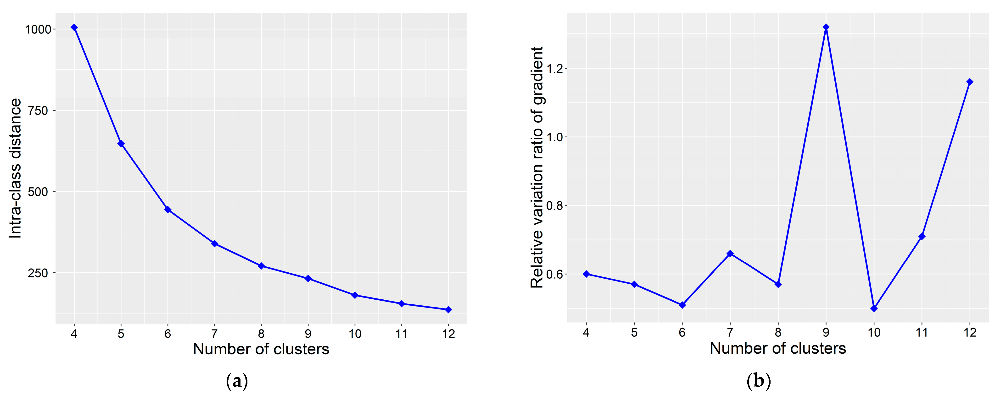
3.4. Determination of K

Section 3.2 and Section 3.3 both depend on the given $K$. From objective function (2), it is shown that for any given $K$, the value of loss function can be calculated, which represents the intra-class error. The “elbow point” of loss function $J\left(K\right)$ is usually used as the optimal number of clusters in literature. The traditional methods treat the maximum point of the second-order difference of $J\left(K\right)$ (i.e., $J\left(K-1\right)-2J\left(K\right)+J\left(K+1\right)$, which describes the absolute variation of first-order difference as the “elbow point”. The minimum point of the ratio of first-order difference (which describes the relative variation of first-order difference) is considered as the “elbow point”; that is,

$$K^{*}=\underset{K_{\min }\le K\le K_{\max }}{\mathrm{argmin}}\frac{J\left(K+1\right)-J\left(K\right)}{J\left(K\right)-J\left(K-1\right)}$$

(7)

where $K_{min}$ and $K_{max}$ are the minimum and maximum of $K$ according to expertise. Equation (7) shows that the optimal number of clusters $K^{*}$ can minimize the relative descent rate of intra-class distance $J\left(K\right)$. Generally speaking, the timescales of one day should be divided into at least four intervals: morning, noon, afternoon, and evening periods; that is, $K_{min}\ge 4$. Additionally, it should never exceed 12 intervals in reality; that is, $K_{max}\le 12$.

3.5. Adjustment of Breakpoints

For the purpose of TIP for traffic signal control, the breakpoints $A_1,\dots ,A_K$ from clustering results could not be optimal. To fix this, the breakpoints between clusters are updated repeatedly, until convergence, according to the following formulas.

$$A_1\leftarrow A_1+\frac{1}{T}I[\left({\overline{y}}_{\left(1\right)}-y_{\left[A_K\right]}\right)\left({\overline{y}}_{\left(1\right)}-{\overline{y}}_{\left(K\right)}\right)<0\left]-\frac{1}{T}I\right[\left({\overline{y}}_{\left(K\right)}-y_{\left[A_K\right]}\right)\left({\overline{y}}_{\left(K\right)}-{\overline{y}}_{\left(1\right)}\right)<0]$$

(8)

$$A_k\leftarrow A_k+\frac{1}{T}I\left[\left({\overline{y}}_{\left(k\right)}-y_{\left[A_{k-1}\right]}\right)\left({\overline{y}}_{\left(k\right)}-{\overline{y}}_{\left(k-1\right)}\right)<0\right]-\frac{1}{T}I[\left({\overline{y}}_{\left(k-1\right)}-y_{\left[A_{k-1}\right]}\right)\left({\overline{y}}_{\left(k-1\right)}-{\overline{y}}_{\left(k\right)}\right)<0]$$

(9)

for $2\le k\le K$ where ${\overline{y}}_{\left(k\right)}={[{\displaystyle \sum }_{j=1}^{T}I\left(c_j^i=k\right)]}^{-1}{\displaystyle \sum }_{j=1}^{T}I\left(c_j^i=k\right)y_j$ represents the average traffic flow of the k-th cluster, $y_{\left[A_k\right]}=y_j\left(j:A_k=B_j\right)$ represents the traffic flow at breakpoint $A_k$.

More specifically, if the traffic flow at breakpoint $A_k$ is less than the average traffic flow of its left cluster ${\overline{y}}_{\left(k-1\right)}$ and also less than the average traffic flow of its right cluster ${\overline{y}}_{\left(k\right)}$, and ${\overline{y}}_{\left(k-1\right)}<{\overline{y}}_{\left(k\right)}$, then $A_k$ should belong to the left cluster. Then, the breakpoint between these two adjacent clusters should move toward right. On the contrary, if the traffic flow at breakpoint $A_k$ is greater than ${\overline{y}}_{\left(k-1\right)}$ and ${\overline{y}}_{\left(k\right)}$, and ${\overline{y}}_{\left(k-1\right)}<{\overline{y}}_{\left(k\right)}$, then $A_{k+1}$ should belong to the right cluster, and the breakpoint should move toward left.

4. Case Study

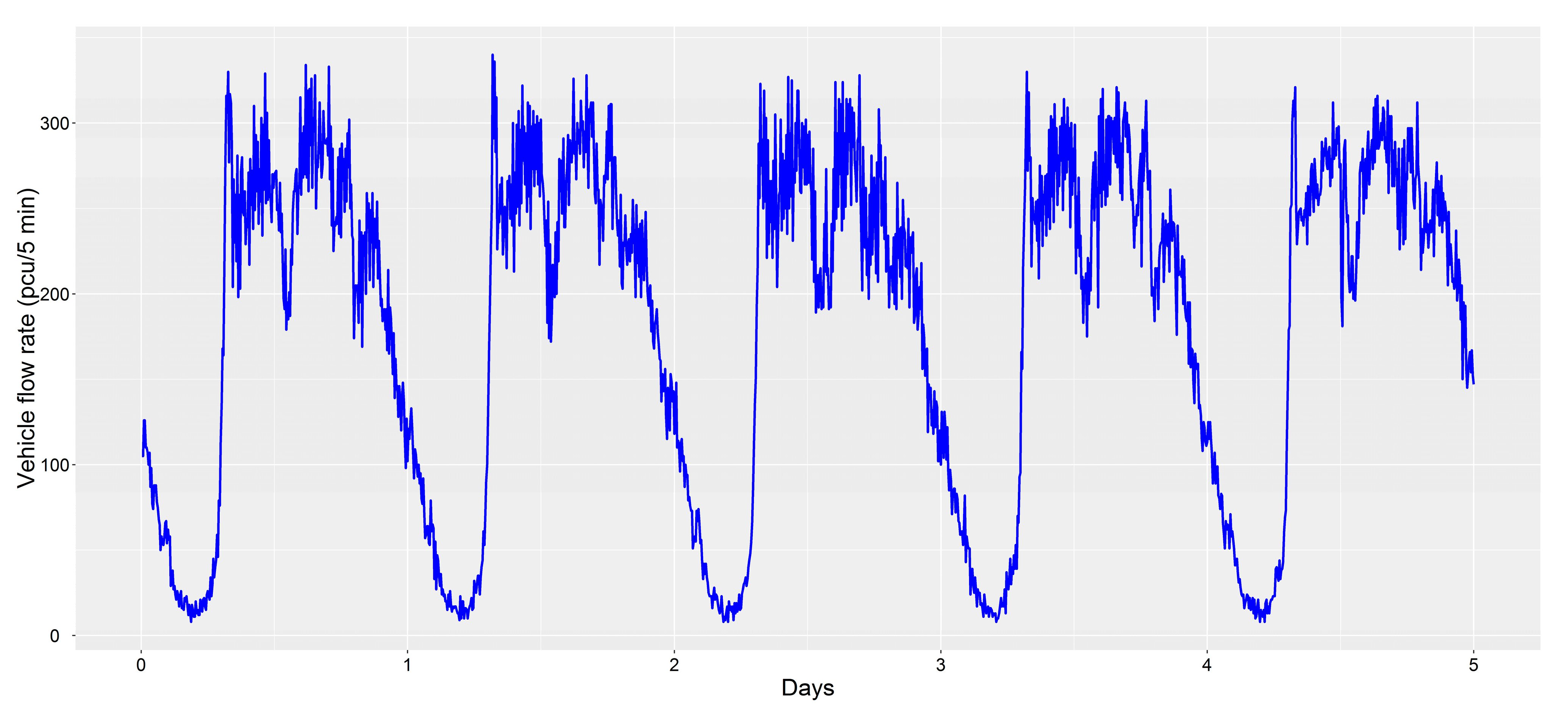
4.1. Empirical Data

The empirical data were collected at the signalized intersection of Wuyi Road and Jintai Street in Fuzhou city, China. There are five lanes in each entrance (lanes 1 and 2 dedicated to left turn vehicles, lanes 3 and 4 for through vehicles, and lane 5 shared by through and right-turning vehicles) and three signal phases at the intersection (phase 1: left turn on north and south entrances; phase 2: through on north and south entrances; phase 3: left turn and through on east and west entrances). Figure 1 manifests the aggregated vehicle flow rate of all five lanes, which is counted every 5 min, from 0:00 on 26 December 2016 to 24:00 on 30 December 2016.

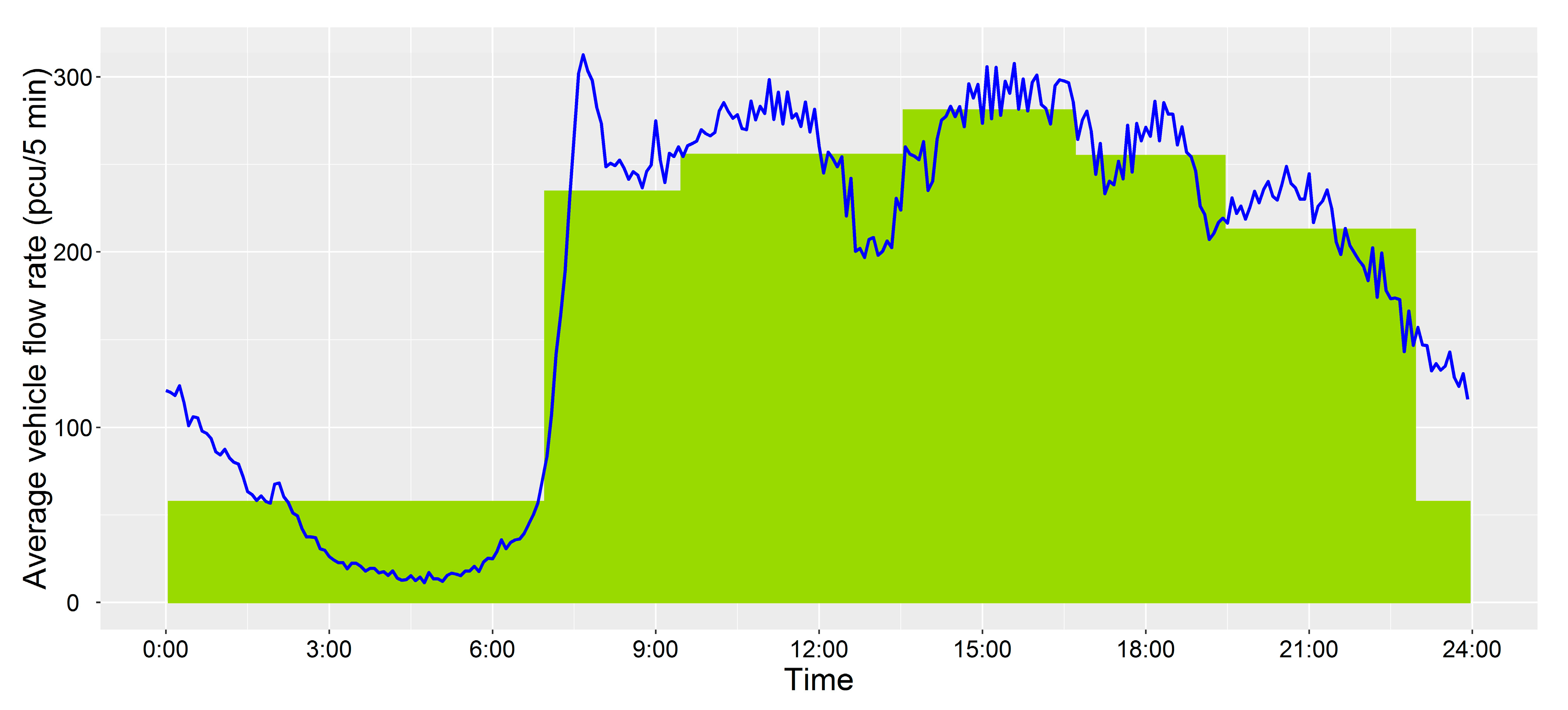
4.2. Results of Clustering

Above all, the proposed “elbow point” method is applied to determine the number of clusters $K$. In Formulas (5) and (6), we set $\delta \left(K\right)=1/\left(3K\right)$, $K_{min}=4$ and $K_{max}=12$. Figure 2a shows the intra-class distances of different numbers of clusters, and Figure 2b shows the relative descent rates of intra-class distance as $K$ increasing.

In Figure 2a, the intra-class distance decreases gradually as $K$ increases and the relative descent rates of intra-class distance are relatively small when $K=6$ or $K=10$ in Figure 2b. In traffic engineering, frequent signal control scheme changes will bring management costs to the transportation department. A smaller $K$ means less overhead, so 6 is chosen as the number of clusters.

Next, the proposed cyclic weighted k-means method is applied, and the breakpoints between time intervals are adjusted according to (8) and (9). Figure 3 demonstrates the clustering results.

The curve in Figure 3 shows the average traffic volume per five minutes (i.e., average traffic flow rate, ATFR; basic unit: pcu/h, passenger car unit per hour) of the intersection in five days, and the ladder shape curve shows the mean of the ATFR in each cluster. These clusters are the morning peak hour (6:55–9:30), forenoon hour (9:30–13:35), afternoon hour (13:35–16:45), evening peak hour (16:45–19:25), night hour (19:25–22:55) and midnight hour (22:55–6:55).

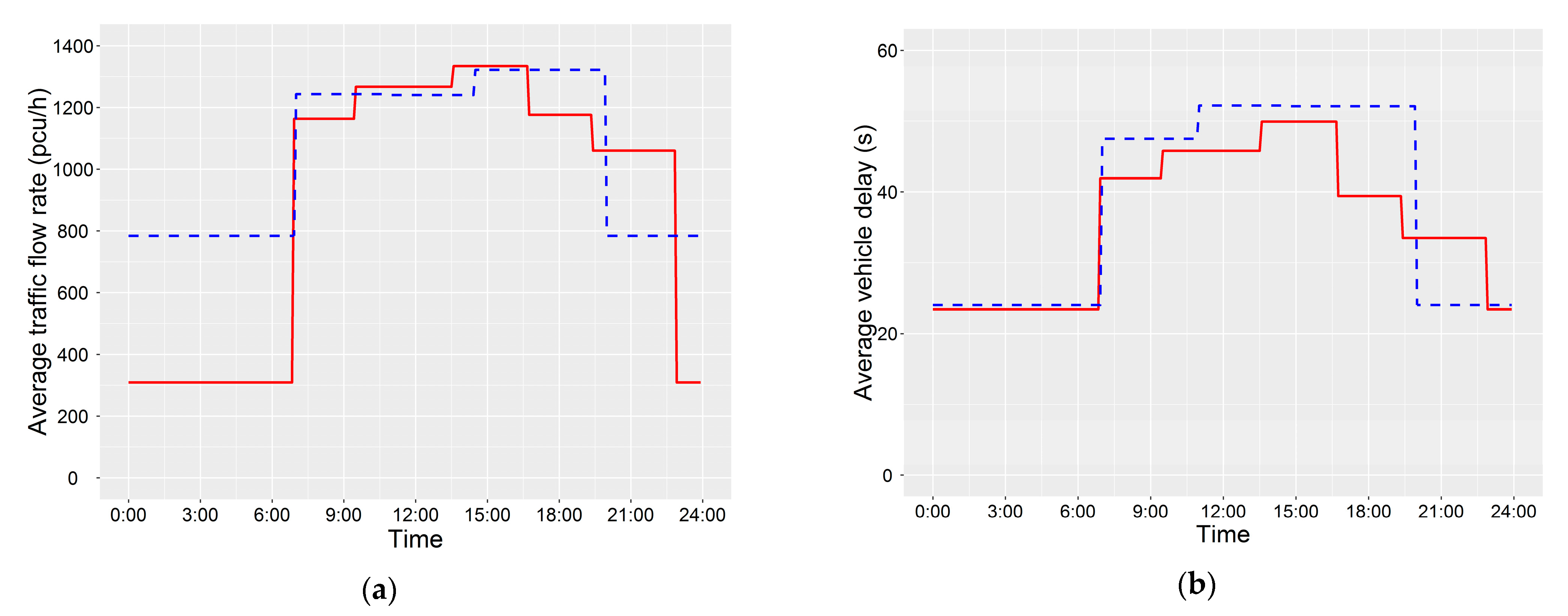
4.3. Evaluation of Methods

To evaluate different TIP methods, a common evaluation index, the average vehicle delay (AVD), was adopted in this study. Details of the AVD method are given in [44,45] and Appendix A.

Two TIP plans are compared, i.e., Plan A (the proposed method) and Plan B (the TIP plan currently used by the local transportation department according to practical experience) via AVD. The whole day is divided into four periods by Plan B as follows, the morning peak hour (7:00–11:00), off-peak hour in the noon (11:00–14:30), the afternoon to the evening peak hour (14:30–20:00), off-peak hour in the night (20:00–7:00). Figure 4a shows the ATFR of these two plans.

According to Webster’s signal control method [46], we partly calculate AVD for each time interval of both two plans, then get AVD of the whole day (see Figure 4b). Note that the ATFR of Plan B in Figure 4a during the second (7:00–11:00) and third (11:00–14:30) periods is in a line, and it is hard to intuitively distinguish (1243 and 1240 pcu/h, respectively). It is the same situation for the third (11:00–14:30) and fourth (14:30–20:00) periods of Plan B in Figure 4b, with AVD 52.2 and 52.1 s.

Figure 4 displays that Plan A is better than Plan B because the AVD of Plan A is always lower than that of Plan B, except from 20:00 to 22:55. However, the ATFR of this period still maintains 1176 pcu/h, an average of about 100 pcu per five minutes. Thus, it is not reasonable for Plan B to regard this period as the night. By further calculation, the AVD for the whole day of the two plans is 35 and 39 s, respectively. It follows that the AVD of Plan A decreases by 10.25% than one of Plan B. We can say that the regular pattern of the traffic flow is accurately captured by Plan A, and the time interval is frequently divided. This brings more benefit for traffic than Plan B, which is designed mainly from engineering experience with a lack of theoretical basis and analysis.

5. Conclusions

For cyclic data, such as traffic flows, a clustering method is proposed, called cyclic weighted k-means, based on cyclic distance. Several conclusions are as follows.

i.

The cyclic distance is the key for the cyclic weighted k-means algorithm, which makes it possible that the end point of the previous cycle and the start point of the current cycle are connected in the clustering result, and a complete cycle of data has been considered rather than separation from tail to head.

ii.

Some attached algorithms, i.e., centroid initialization, cluster number selection, and breakpoint adjustment, are helpful for further improvement of the cyclic weighted k-means algorithm to solve the TIP problem.

iii.

The feasibility of the proposed method is confirmed by empirical study. It is noted that the practical evaluation criteria (such as the average vehicle delay in benefits of traffic signal control) should serve the practice. From the perspective of application, the proposed method can also be applied to other scenes. For example, it can be applied to the inventory adjustment of e-commerce according to the daily sales, and the seat optimization of a call center according to the volume of calls.

From the perspective of application, a novel TIP algorithm (i.e., cyclic weighted k-means) for traffic signal control was developed according to the periodic change of the traffic flow at the signalized intersection. The purpose of the algorithm is to improve the benefits of traffic signal control. On the one hand, traffic flow data can only be obtained by the detectors (such as loop detector or video detector) at intersections. In reality, missing data or sensor damage often occur. Hence, developing a filling method for missing traffic flow data is an important task in future work. On the other hand, traffic flows at intersections show different periodic changes on weekdays, weekends, and holidays, which requires different TIP schemes. The current traffic signal control system can store different TIP schemes for different days and set the optimal signal timing plans for each time interval, which is of great significance to improve the benefits of traffic signal control.

References

- Ma, D.; Luo, X.; Jin, S.; Wang, D.; Guo, W.; Wang, F. Lane-Based Saturation Degree Estimation for Signalized Intersections Using Travel Time Data. IEEE Intell. Transp. Syst. Mag. 2017, 9, 136–148. [Google Scholar] [CrossRef]
- Mirchandani, P.; Head, L. A Real-Time Traffic Signal Control System: Architecture, Algorithms, and Analysis. Transp. Res. Part C: Emerg. Technol. 2001, 9, 415–432. [Google Scholar] [CrossRef]
- Di Febbraro, A.; Giglio, D.; Sacco, N. A Deterministic and Stochastic Petri Net Model for Traffic-Responsive Signaling Control in Urban Areas. IEEE Trans. Intell. Transp. Syst. 2015, 17, 510–524. [Google Scholar] [CrossRef]
- Schmöcker, J.-D.; Ahuja, S.; Bell, M.G. Multi-Objective Signal Control of Urban Junctions—Framework and a London Case Study. Transp. Res. Part C: Emerg. Technol. 2008, 16, 454–470. [Google Scholar] [CrossRef]
- Keyvan-Ekbatani, M.; Yildirimoglu, M.; Geroliminis, N.; Papageorgiou, M. Multiple Concentric Gating Traffic Control in Large-Scale Urban Networks. IEEE Trans. Intell. Transp. Syst. 2015, 16, 2141–2154. [Google Scholar] [CrossRef]
- Papageorgiou, M.; Kiakaki, C.; Dinopoulou, V.; Kotsialos, A.; Wang, Y. Review of Road Traffic Control Strategies. Proc. IEEE 2003, 91, 2043–2067. [Google Scholar] [CrossRef]
- Chang, T.-H.; Lin, J.-T. Optimal Signal Timing for an Oversaturated Intersection. Transp. Res. Part B: Methodol. 2000, 34, 471–491. [Google Scholar] [CrossRef]
- Lertworawanich, P.; Kuwahara, M.; Miska, M. A New Multiobjective Signal Optimization for Oversaturated Networks. IEEE Trans. Intell. Transp. Syst. 2011, 12, 967–976. [Google Scholar] [CrossRef]
- Liu, Z.; Bie, Y. Comparison of Hook-Turn Scheme with U-Turn Scheme Based on Actuated Traffic Control Algorithm. Transp. A Transp. Sci. 2015, 11, 484–501. [Google Scholar] [CrossRef]
- Zhao, L.; Peng, X.; Li, L.; Li, Z. A Fast Signal Timing Algorithm for Individual Oversaturated Intersections. IEEE Trans. Intell. Transp. Syst. 2010, 12, 280–283. [Google Scholar] [CrossRef]
- Bie, Y.; Liu, Z. Evaluation of a Signalized Intersection with Hook Turns under Traffic Actuated Control Circumstance. J. Transp. Eng. 2015, 141, 04014093. [Google Scholar] [CrossRef]
- Bie, Y.; Gong, X.; Liu, Z. Time of Day Intervals Partition for Bus Schedule Using GPS Data. Transp. Res. Part C Emerg. Technol. 2015, 60, 443–456. [Google Scholar] [CrossRef]
- Chen, P.; Zheng, N.; Sun, W.; Wang, Y. Fine-Tuning Time-of-Day Partitions for Signal Timing Plan Development: Revisiting Clustering Approaches. Transp. A Transp. Sci. 2019, 15, 1195–1213. [Google Scholar] [CrossRef]
- Murphy, K.P. Machine Learning: A Probabilistic Perspective; The MIT Press: Cambridge, MA, USA; London, UK, 2012. [Google Scholar]
- Dempster, A.P.; Laird, N.M.; Rubin, D.B. Maximum Likelihood from Incomplete Data via the EM Algorithm. J. R. Stat. Soc. Ser. B Methodol. 1977, 39, 1–22. [Google Scholar]
- Wu, C.F.J. On the Convergence Properties of the EM Algorithm. Ann. Stat. 1983, 11, 95–103. [Google Scholar] [CrossRef]
- Fraley, C.; Raftery, E.A. Model-Based Clustering, Discriminant Analysis, and Density Estimation. J. Am. Stat. Assoc. 2002, 97, 611–631. [Google Scholar] [CrossRef]
- Frey, B.J.; Dueck, D. Clustering by Passing Messages between Data Points. Science 2007, 315, 972–976. [Google Scholar] [CrossRef] [PubMed]
- Rodriguez, A.; Laio, A. Clustering by Fast Search and Find of Density Peaks. Science 2014, 344, 1492–1496. [Google Scholar] [CrossRef]
- Huang, W.; Cao, X.; Biase, F.H.; Yu, P.; Zhong, S. Time-Variant Clustering Model for Understanding Cell Fate Decisions. Proc. Natl. Acad. Sci. USA 2014, 111, E4797–E4806. [Google Scholar] [CrossRef]
- Shah, S.A.; Koltun, V. Robust Continuous Clustering. Proc. Natl. Acad. Sci. USA 2017, 114, 9814–9819. [Google Scholar] [CrossRef]
- Smith, B.L.; Scherer, W.T.; Hauser, T.A. Data-Mining Tools for the Support of Signal-Timing Plan Development. Transp. Res. Rec. J. Transp. Res. Board 2001, 1768, 141–147. [Google Scholar] [CrossRef]
- Ratrout, N.T. Developing Optimal Timing Plans for Cyclic Traffic along Arterials Using Pre-Timed Controllers. Proc. Urban Trans. 2011, 116, 367. [Google Scholar]
- Ratrout, N.T. Subtractive Clustering-Based K-means Technique for Determining Optimum Time-of-Day Breakpoints. J. Comput. Civ. Eng. 2011, 25, 380–387. [Google Scholar] [CrossRef]
- Xia, J.; Chen, M. Defining Traffic Flow Phases Using Intelligent Transportation Systems-Generated Data. J. Intell. Transp. Syst. 2007, 11, 15–24. [Google Scholar] [CrossRef]
- Wang, X.; Cottrell, W.D.; Mu, S. Using K-Means Clustering to Identify Time-of-Day Break Points for Traffic Signal Timing Plans. In Proceedings of the 2005 IEEE Intelligent Transportation Systems, Vienna, Austria, 16 September 2005; pp. 586–591. [Google Scholar]
- Guo, R.; Zhang, Y. Identifying Time-of-Day Breakpoints Based on Nonintrusive Data Collection Platforms. J. Intell. Transp. Syst. 2013, 18, 164–174. [Google Scholar] [CrossRef]
- Dong, C.; Su, Y.; Liu, X. Research on TOD Based on Isomap and K-means Clustering Algorithm. In Proceedings of the 2009 Sixth International Conference on Fuzzy Systems and Knowledge Discovery, Tianjin, China, 14–16 August 2009; Volume 1, pp. 515–519. [Google Scholar]
- Ma, D.; Li, W.; Song, X.; Wang, Y.; Zhang, W. Time-of-Day Breakpoints Optimisation through Recursive Time Series Partitioning. IET Intell. Transp. Syst. 2019, 13, 683–692. [Google Scholar] [CrossRef]
- Lee, J.; Kim, J.; Park, B. A Genetic Algorithm-Based Procedure for Determining Optimal Time-of-Day Break Points for Coordinated Actuated Traffic Signal Systems. KSCE J. Civ. Eng. 2010, 15, 197–203. [Google Scholar] [CrossRef]
- Park, B.; Santra, P.; Yun, I.; Lee, D.-H. Optimization of Time-of-Day Breakpoints for Better Traffic Signal Control. Transp. Res. Rec. J. Transp. Res. Board 2004, 1867, 217–223. [Google Scholar] [CrossRef]
- Park, B.; Lee, H.; Yun, I. Enhancement of Time of Day Based Traffic Signal Control. In Proceedings of the 2003 IEEE International Conference on Systems, Man and Cybernetics, Washington, DC, USA, 8 October 2003. [Google Scholar] [CrossRef]
- Yang, J.; Yang, Y. Using Kohonen Cluster to Identify Time-of-Day Break Points of Intersection. Lect. Notes Electr. Eng. 2013, 236, 889–896. [Google Scholar]
- Jia, L.; Yang, L.; Kong, Q.; Lin, S. Study of Artificial Immune Clustering Algorithm and its Applications to Urban Traffic Control. Int. J. Inf. Technol. 2006, 12, 1–6. [Google Scholar]
- Erman, J.; Arlitt, M.; Mahanti, A. Traffic Classification using Clustering Algorithms. In Proceedings of the 2006 Sigcomm Workshop on Mining Network Data-MineNet ’06; ACM: Nashville, TN, USA, 2006; pp. 281–286. [Google Scholar]
- Michalopoulos, P.G.; Stephanopoulos, G. Oversaturated Signal Systems with Queue Length Constraints—I: Single Intersection. Transp. Res. 1977, 11, 413–421. [Google Scholar] [CrossRef]
- Ban, X.; Hao, P.; Sun, Z. Real Time Queue Length Estimation for Signalized Intersections using Travel Times from Mobile Sensors. Transp. Res. Part C Emerg. Technol. 2011, 19, 1133–1156. [Google Scholar] [CrossRef]
- Farahani, R.Z.; Miandoabchi, E.; Szeto, W.; Rashidi, H. A Review of Urban Transportation Network Design Problems. Eur. J. Oper. Res. 2013, 229, 281–302. [Google Scholar] [CrossRef]
- Bräysy, O.; Gendreau, M. Vehicle Routing Problem with Time Windows, Part I: Route Construction and Local Search Algorithms. Transp. Sci. 2005, 39, 104–118. [Google Scholar] [CrossRef]
- Calderón, F.; Miller, E.J. Modelling within-Day Ridehailing Service Provision with Limited Data. Transp. B Transp. Dyn. 2021, 9, 62–85. [Google Scholar] [CrossRef]
- Wang, S.; Zhang, W.; Bie, Y.; Wang, K.; Diabat, A. Mixed-Integer Second-Order Cone Programming Model for Bus Route Clus-tering Problem. Trans. Res. Part C Emerg. Technol. 2019, 102, 351–369. [Google Scholar] [CrossRef]
- Bie, Y.; Hao, M.; Guo, M. Optimal Electric Bus Scheduling Based on the Combination of All-Stop and Short-Turning Strategies. Sustainability 2021, 13, 1827. [Google Scholar] [CrossRef]
- Crainic, T.G.; Gendreau, M.; Potvin, J.-Y. Intelligent Freight-Transportation Systems: Assessment and the Contribution of Op-erations Research. Trans. Res. Part C Emerg. Technol. 2009, 17, 541–557. [Google Scholar] [CrossRef]
- Gordon, R.L.; Tighe, W. Traffic Control Systems Handbook; FHWA Office of Operations: Washington, DC, USA, 2005. [Google Scholar]
- Klein, L.A.; Gibson, D.; Mills, M.K. Traffic Detector Handbook; Federal Highway Admin: Washington, DC, USA, 2006. [Google Scholar]
- Webster, F. Traffic Signal Settings. In Road Research Technique Paper No. 39; Road Research Laboratory: London, UK, 1958. [Google Scholar]
- Wang, L.; Wang, Y.; Bie, Y. Automatic Estimation Method for Intersection Saturation Flow Rate Based on Video Detector Data. J. Adv. Transp. 2018, 2018, 1–9. [Google Scholar] [CrossRef]
- Council, N.R. Highway Capacity Manual; Transportation Research Board: Washington, DC, USA, 2000. [Google Scholar]
Publisher’s Note: MDPI stays neutral with regard to jurisdictional claims in published maps and institutional affiliations. |
© 2021 by the authors. Licensee MDPI, Basel, Switzerland. This article is an open access article distributed under the terms and conditions of the Creative Commons Attribution (CC BY) license (https://creativecommons.org/licenses/by/4.0/).
Share and Cite
Wang, G.; Qin, W.; Wang, Y. Cyclic Weighted k-means Method with Application to Time-of-Day Interval Partition. Sustainability 2021, 13, 4796. https://doi.org/10.3390/su13094796
Wang G, Qin W, Wang Y. Cyclic Weighted k-means Method with Application to Time-of-Day Interval Partition. Sustainability. 2021; 13(9):4796. https://doi.org/10.3390/su13094796
Chicago/Turabian StyleWang, Gaizhen, Wei Qin, and Yunhao Wang. 2021. "Cyclic Weighted k-means Method with Application to Time-of-Day Interval Partition" Sustainability 13, no. 9: 4796. https://doi.org/10.3390/su13094796
APA StyleWang, G., Qin, W., & Wang, Y. (2021). Cyclic Weighted k-means Method with Application to Time-of-Day Interval Partition. Sustainability, 13(9), 4796. https://doi.org/10.3390/su13094796