Abstract
Evaluating the life cycle of buildings is a valuable tool for assessing sustainability and analyzing environmental consequences throughout the construction operations of buildings. In this study, in order to determine the importance of building life cycle evaluation indicators, a new combination method was used based on a quantitative-qualitative method (QQM) and a simplified best-worst method (SBWM). The SBWM method was used because it simplifies BWM calculations and does not require solving complex mathematical models. Reducing the time required to perform calculations and eliminating the need for complicated computer software are among the advantages of the proposed method. The QQM method has also been used due to its ability to evaluate quantitative and qualitative criteria simultaneously. The feasibility and applicability of the SBWM were examined using three numerical examples and a case study, and the results were evaluated. The results of the case study showed that the criteria of the estimated cost, comfort level, and basic floor area were, in order, the most important criteria among the others. The results of the numerical examples and the case study showed that the proposed method had a lower total deviation (TD) compared to the basic BWM. Sensitivity analysis results also confirmed that the proposed approach has a high degree of robustness for ranking and weighting criteria.
1. Introduction
Life cycle assessment (LCA) is a systematic approach to analyzing and evaluating the environmental impact of a product or process throughout its life cycle. LCA typically involves the major stages of extraction, production, use, and end-of-life material scenarios for a product or process. LCA is a four-step iterative process that includes setting goals and scope, life-cycle inventory (LCI), life-cycle impact assessment (LCIA), and interpretation [1]. The LCI stage is often where the LCA ends due to a developmental, mental, and framework mismatch in the LCIA stage. There are two ways to generate LCI. The process method systematically calculates known environmental inputs and outputs using process flow diagrams. The scope of the process model continues to the extent that the flow between the process and the diffusion is negligible [2].
The building sector has significant environmental impacts and is responsible for a remarkable portion of the world’s energy and resource consumption [3]. The overall goal of building life cycle assessment is multifaceted and includes minimizing environmental impacts, carbon emissions, energy, and costs [4]. Evaluating the life cycle of buildings is a widely recognized environmental management method [5]. It has been attempted to assess the environmental impact of buildings, their constituents, components, and systems and to examine every opportunity to reduce their environmental impact [6]. As an alternative to building environmental assessment schemes, building life cycle assessments can assess the environmental impact of a building based on a number of known impact factors. Due to its comprehensive coverage of environmental impacts and computational effectiveness, evaluating the life cycle of buildings has been widely accepted as a tool to support decision-making at both the commercial and political levels [7]. Improving energy efficiency is a very effective way to achieve emission reduction goals; the accurate assessment of the life cycle of buildings is one of the ways to guide the proper management of resources [8]. Moreover, considering global warming, it is necessary to consider the design of resource monitoring and evaluation systems throughout the supply chain [9].
In recent years, many studies have been conducted on evaluating the life cycle of buildings [10,11]. Evaluating the life cycle of buildings consists of four interrelated stages: brief, design, construction, and maintenance [12].
Mathematical models have been widely used in many fields of science and industry and researchers have developed many mathematical models for various purposes. Many mathematical models have been developed in the field of decision-making and have been used to solve various managerial and decision-making problems. Given the increasing complexity of organizations and firms, improving the decision-making process has become inevitable in various organizations. Various mathematical and computational methods and models have been proposed to help decision-makers (DMs), each with their own characteristics. Some researchers have proposed special criteria for recognizing a good model, including the accuracy of the model results, ease of understanding the model, the time required for modeling and running the model, and the hardware (e.g., computer memory) needed to solve the model. The 14th-century philosopher Ockham states that “it is vain to do more than what can be done by fewer”—his means we should use the simplest model that achieves the goals [13].
Multi-criteria decision-making (MCDM) is a methodology that is able to simultaneously take into account a large number of criteria for the decision-making process and select the appropriate option based on the information and preferences of the DMs [14]. When there are a large number of measures to solve decision problems, especially in cases in which the measures conflict with each other, MCDM is very helpful for researchers and DMs [15]. In various decision-making scenarios in MCDM, there are often three main processes: ranking, sorting, and choice [16].
Due to the multidimensionality of the objectives in sustainability assessment issues and the complexity of these issues, MCDM methods have become increasingly popular [17]. MCDM is not only a method but also includes the planning, goals, and consequences of the decision process [18]. One of the important features that has expanded the scope of use of MCDM methods is the very high flexibility of these methods when dealing with simultaneous quantitative and qualitative criteria in the decision-making process [19]. In recent years, there have been new developments in MCDM methods so that the use of these methods has led to significant growth in infrastructure management programs and construction projects. It has also been reported that many decision support tools based on MCDM methods have been used successfully for infrastructure management and construction projects [20]. There are several quantitative and qualitative criteria for evaluating the life cycle of buildings. To obtain the importance of qualitative criteria, some limitations are often set to increase the accuracy of the analysis of hypotheses and data of decision problems [21]. In these cases, the importance of the criteria can be obtained using MCDM methods based on pairwise comparisons and the preferences determined by the experts. The goal of MCDM methods is to achieve a combination of different forms of input data needed to define and analyze complex decision problems [22].
Due to the ability of MCDM methods to make a comprehensive evaluation of the parameters and variables affecting the decision process, researchers and decision-makers use MCDM techniques for assessing the life cycle of buildings and various management issues. For example, the combination of AHP (analytical hierarchy process), which is one of the most well-known methods of MCDM, and the LCA method has been used to evaluate the sustainability of energy systems [23]. In a study, a combination of two methods—analytic network process (ANP) and benefit, opportunity, cost, risk (BOCR)—was used for planning and managing renewable resources in Iran and, based on the results, it was found that solar energy was the most important renewable energy source in that country [24]. The combination and integration of new methodologies makes it possible to use their advantages simultaneously and achieve the most accurate and robust results for various decision-making issues [25].
The best-worst method (BWM) was introduced by Rezaei [26] as a MCDM method. In this method, first some criteria are selected to perform the decision-making process, and then the best criterion (the most important criterion from DM’s point of view) and the worst criterion (the least important criterion from DM’s point of view) are selected. The criteria are then compared with the best and worst criteria in a pairwise comparison, so decision-maker (DM) preferences are identified at this stage. Then, based on the pairwise comparisons and DM preferences, a linear programming model is formed and by solving it, the optimal weight each criterion is determined. Obviously, with the increase in the number of criteria and the complexity of calculations, it is not possible to solve the programming model manually, and its solving requires optimization software. Therefore, it is necessary to develop software packages to reduce computational complexity [27]. Despite the challenges facing BWM, its advantages have always attracted the attention of researchers. Reducing the number of comparisons can be the most important advantage of BWM over other existing methods such as AHP. Reducing the number of comparisons has made it easier to gather information and increased the consistency and accuracy of the results of this method [28].
The quantitative-qualitative method (QQM) is a method for the simultaneous evaluation of quantitative and qualitative criteria that has a high ability to obtain the final weight of the criteria when obtaining the importance of decision criteria in a situation where there are a number of quantitative and qualitative [12]. In this method, seven steps are taken to determine the importance of the criteria. The importance of the quantitative criteria is specified in Steps 1–4, and that of the qualitative criteria is calculated in Steps 5–7, which are described in the Methodology Section.
The main purpose of this paper is to provide a combined approach based on simplified computational BWM and QQM that will help researchers and DMs deal with decision-making issues in the life cycle of buildings. BWM has an important place in decision-making research due to its advantages over previous pairwise comparison-based methods. In this paper, a computational approach is introduced based on the simplified best-worst method (SBWM), which calculates the decision-making criteria weights using simpler calculations and without the need to solve the linear programming model. In the original BWM, after pairwise comparisons by DMs, the linear programming model is formulated and solved to determine the optimal weights of the decision criteria. However, in this paper, the SBWM calculates the weights of the criteria without the need to create a programming model and it has simpler calculations. It is very important to provide a fast and accurate computational method that provides robust results and helps decision-makers in various decision issues [29]. The advantages of the proposed methods include: ease of understanding the method, improvement of the results accuracy, ease of the model solving, reducing the complexity of calculations, and there is no need for software or even a computer.
Solving large-scale linear programming models often requires the use of software packages. Therefore, researchers need to have sufficient skills to work with relevant software. Being able to calculate the answer of linear models manually can be an important advantage, especially when the relevant software packages are not available. SBWM is a modified form of the basic BWM that allows the weights of any number of criteria to be obtained by solving only a few equations, and, unlike BWM, it does not require the use of a software package. SBWM was used to evaluate the life cycle of buildings and the results were compared with the results of QQM. It was then demonstrated how the results of the two methods can be combined. Our research contributions can be summarized as follows:
- A modified version of BWM is provided, which has simpler calculations compared to the original model and does not require complex mathematical models and special software packages;
- In the new SBWM, we propose mathematical relationships to calculate the consistency index of decision-makers’ preferences as well as to determine the source of inconsistency (SI);
- The SBWM is described using three numerical examples, and the hybrid QQM-SBWM approach is used to evaluate the life cycle of buildings, and the advantages of both methods are described;
- Sensitivity analysis is used to evaluate the robustness of the results of the proposed approach;
- A decision support framework is provided for various decision issues that have both quantitative and qualitative criteria.
The rest of the paper is organized as follows: Section 2 provides an in-depth review of BWM developments. Section 3 presents the steps of the basic BWM, SBWM, and QQM. In Section 4, the SBWM is used in numerical examples and the results are compared with the results of the original BWM. Section 5 analyzes the sensitivity of the results obtained by SBWM. In Section 6, a determination of the importance of building life cycle assessment criteria is provided. Finally, in Section 7, conclusions and some suggestions for future research are provided.
2. Survey on the Developments of the BWM
In this section, some applications and developments of the BWM were reviewed in order to identify the research gap and design the main research question. To accurately assess the development of BWM and the features that have been added to BWM over time, it is necessary to carefully review the studies conducted in this area; here, we mention some of the most important studies in this area.
BWM is a new MCDM technique introduced by Rezaei [26]. It is based on pairwise comparisons of all criteria with the best and worst criteria, which are known as reference comparisons. Then, a programming model is formed based on comparisons made by DMs, and the optimal weights of the criteria are obtained by solving it. BWM requires fewer pairwise comparisons than the AHP, so less information is needed to make decisions, and on the other hand, it provides more consistent results. These features make it an efficient tool for DMs. In the following, some of the BWM applications in various fields and, more importantly, some of studies that have developed and improved BWM are reviewed. BWM was used to rank and prioritize alternatives or to obtain criteria weights in decision-making and other fields including: supplier selection [30,31,32,33,34,35], performance evaluation [36,37,38,39], intelligent product service systems [40], cloud service selection [41], prioritization of barriers of big data adoption [42], repair unit evaluation [43], site selection [44,45], project selection [46], locating and evaluating the charging stations [47,48], prioritization of failure cases [49], personnel selection [50], assessment of third-party logistics provider [51], prospectivity mapping [52], energy [53], and many other areas.
The following is a summary of some of the studies conducted on the development of BWM.
Rezaei [54] introduced a linear programming model for BWM. In the original BWM model, after making pairwise comparisons between the criteria, the Min-Max model is formulated and solved to obtain the weights of the decision criteria. Because this model is nonlinear, there may be several optimal solutions, while some DMs tend to obtain only one optimal solution for their decision-making problem. Guo and Zhao [55] developed BWM to make decisions in a triangular fuzzy environment. DMs’ preferences were used in linguistic terms and triangular fuzzy numbers were used as inputs for the model. They used three case study cases to demonstrate the effectiveness and usability of the proposed model. The results showed that fuzzy BWM, in addition to the logical prioritization of alternatives, also provides more compatible comparisons than the original BWM. Mou et al. [56] introduced a new multi-criteria group decision-making method using the logic of intuitionistic fuzzy analytic hierarchy process (IFAHP) and BWM. Intuitionistic fuzzy BWM (IF-BWM) was developed using intuitionistic fuzzy preference relation (IFPR) and a special algorithm. Different mathematical models were proposed to obtain the weights of the criteria, and finally the numerical method was evaluated using three numerical examples. Pamučar et al. [57] expanded BWM using interval-valued fuzzy-rough numbers (IVFRN). For this purpose, a new multi-criteria model was proposed based on IVFRN. The applicability of the proposed method was investigated using a study on the selection of firefighting helicopters. The results showed that their proposed method covered the uncertain conditions in a better manner compared to the traditional fuzzy and rough approaches. Aboutorab et al. [58] developed a z-number version of the BWM which enabled the BWM to control uncertain information in MCDM. Additionally, when the DMs’ preferences are not completely reliable, their method can be helpful, as they evaluated the applicability of the proposed approach for supplier development. Li et al. [59] introduced new MCDM methods based on the dominance degree of probabilistic hesitant fuzzy elements (PHFEs) and BWM using probabilistic hesitant fuzzy information. Then, they extended BWM to fuzzy preference relations based on the constructed dominance degree matrix. They developed an algorithm to select the best and worst criteria weights and calculated other weights using two new models. Finally, to show the capabilities of the proposed methods, they applied it to select the best investment company among other alternatives and analyzed the results. Hafezalkotob and Hafezalkotob [60] investigated the fuzzy BWM for group decision-making using two linear programming models. A final decision was made based on a combination of opinions of senior DM and experts. Safarzadeh et al. [61] developed BWM for group decision-making using two mathematical models. The output of the models consisted of weights obtained by combining the opinions of the DMs. A comprehensive sensitivity analysis was performed for the main parameters. Finally, the group BWM was evaluated using a real case study. Mohammadi and Rezaei [62] used Bayesian BWM to obtain the weights of decision-making criteria in group decision-making. Their Bayesian BWM calculated the final weights of criteria based on the opinions of a group of DMs. They also proposed a new ranking scheme called Credal Rankings for ranking the decision criteria. Their model calculated the distribution of the weights determined by all DMs. They evaluate the proposed approach using a numerical example. Tabatabaei et al. [63] developed BWM as an integrated model for a decision-making process in which the decision-making group involved a group leader and several members. Their pairwise comparisons were more consistent compared to the original BWM. Additionally, they used two numerical examples and analyzed the results. Pamučar et al. [51] introduced a new integrated interval rough number (IRN) model based on BWM and weighted aggregated sum product assessment (WASPAS) and multi-attributive border approximation area comparison (MABAC). IRN-BWM was used to obtain the weights of the criteria while IRN-WASPAS and IRN-MABAC were used for the final ranking of third-party logistics providers. They used a numerical example to evaluate and demonstrate the feasibility of the model.
Tabatabaei et al. [64] introduced the hierarchical BWM. The model was created for a decision-making situation that requires the calculation of the weights of criteria and sub-criteria, so that for hierarchical decision-making problems, the weights of criteria and sub-criteria are calculated by running the model only once. Liao et al. [65] applied BWM to evaluate hospital performance using hesitant fuzzy linguistic information. The proposed approach made it possible to consider several possible values for DMs’ preferences and include uncertainty in a more tangible manner. Karimi et al. [43] formulated BWM based on a fully fuzzy linear mathematical model for evaluating repairs in hospitals. In their model, it was not necessary to perform all possible comparisons. In other words, only reference comparisons were sufficient. Their reference comparisons included the evaluation of the fuzzy priority of the best criterion over each of the other criteria and fuzzy priority of each criterion over the worst criterion. After that, a fully fuzzy linear mathematical model was used to determine the weights of the criteria. Ijadi et al. [66] extended BWM based on a hierarchical group decision-making algorithm in a fuzzy environment using the principles of axiomatic design. Then, they evaluated the proposed approach using a real decision-making scenario. Brunelli and Rezaei [67] mathematically examined BWM and added a new metric to the overall BWM framework. This metric did not change the original idea of BWM but provided a stronger mathematical logic and eventually led to the creation of an optimization problem that could be linearized and solved. Wu et al. [68] developed BWM based on interval type-2 fuzzy sets (IT2FSs) to solve the problem of group decision-making for green supplier selection. They also used a practical example to evaluate the feasibility of the new method and analyzed the sensitivity of the results. Mou et al. [69] introduced a new BWM-based group decision-making model for uncertain conditions. They developed the intuitionistic fuzzy multiplicative best-worst method (IFMBWM) using intuitionistic fuzzy multiplicative preference relations (IFMPRs) for multi-criteria group decision-making and used the proposed approach to address health management problems.
A multi-objective linear programming model was proposed for the strategic and tactical planning of the bioethanol supply chain, in which the demand for bioethanol was predicted using the ANN artificial neural network. To solve the proposed multi-objective model, a combined approach based on BWM and the Torabi-Hosseini (TH) method was proposed to find the best solution. Then, a real case study was conducted in Iran. The results showed that applying an appropriate policy for distribution of ethanol can lead to a 33% reduction in costs [70]. The hesitant fuzzy best-worst method (HFBWM) was introduced to make decisions in uncertain conditions using hesitant fuzzy preferential relationships. Reference comparisons of the best and worst criteria were made using linguistics terms that included DMs’ hesitant fuzzy preferences. Three case studies were used to demonstrate the capabilities of the proposed method, and the results showed that HFBWM provided more consistent and accurate weights and ranks compared to the original BWM [71]. Given that there are some deficiencies in the ANP network analysis process, a new method based on BWM and ANP network analysis process (called BWANP) was introduced. The proposed method provided more reliable final weights and also reduced the number of pairwise comparisons. Furthermore, in order to increase the accuracy of the decisions and the final rankings, the BWANP method was examined in uncertain conditions and the capabilities of the proposed method were evaluated using a numerical example [72]. Amiri and Emamat [73] proposed two models based on nonlinear BWM and linear BWM. In the proposed models, the number of constraints was reduced to 2n-2, in which n represents the number of criteria. In their research, the capability of the proposed models was demonstrated using a numerical example and the total deviation (TD) of the proposed models was compared with the TD obtained from nonlinear BWM and linear BWM. The proposed models reduced computational complexity and also provided a good overall deviation. Amiri et al. [74] proposed several linear programming models based on BWM and possibilistic chance-constrained programming (PCCP) for weighting and evaluating the decision criteria. The proposed models are based on three measures of possibility, necessity, and credibility, which are parts of PCCP and allow the decision-makers to take into account uncertainties in the calculation of weights as well as include their optimistic, pessimistic, and intermediate attitudes in determining the weight of decision criteria.
Amiri et al. [28] introduced integrated fuzzy models based on BWM and fuzzy preference programming for weighting and evaluating the decision criteria. Their proposed models could be used in individual and group decision-making. One of the advantages of these models is that there was no need to calculate the consistency rate of the experts’ opinions separately; in their models, the consistency rate of the comparisons is determined by the model. They evaluated hospital performance in a real case study to evaluate the proposed approach.
According to the studies reviewed above, it is clear that BWM has been well-considered by researchers and has had various applications in various fields of science. The advantages of BWM (such as needing less information for the decision-making process, fewer pairwise comparisons, providing robust results, and a high consistency rate) has made this method one of the most popular multi-criteria decision-making methods in recent years. Now, the research gap is how to perform calculations in this method more easily and achieve the final results more quickly. Developing BWM in such a way that we can achieve acceptable results as easily as possible without the need for a complex computing platform and linear programming can increase the advantages of the method and add new features to its previous model.
In this study, it is hypothesized that simplified BWM can be developed to deal with various decision-making problems in a way that we can obtain the final weights of decision criteria without the need for complex linear and nonlinear programming models. Therefore, the main research question is: how can we develop BWM so that it can be applied to various decision-making problems without having to solve programming models?
In this article, we aim to provide a combined method based on a simpler computational method for calculating the weights or ranking the alternatives and QQM.
3. Methodology
In this section, first the steps of the BWM method are described, then the steps of the SBWM method are reviewed and analyzed, and finally the QQM is introduced. The steps of the proposed approach are briefly shown in Figure 1.
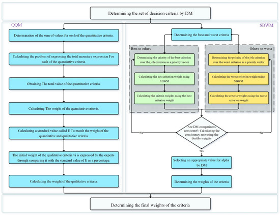
Figure 1.
The framework of QQM-SBWM.
3.1. The BWM
The mathematical formulation proposed in this study is based on BWM reference comparisons and creates a decision platform that can be solved without the need for software and reduces computational time. BWM uses reference comparisons and creates two preference vectors: priorities of the best criterion over the rest of the criteria and priorities of all criteria over the worst criterion (see Figure 2); then a linear or nonlinear programming model is used to determine the weights and ranks. The steps of basic BWM are as follows:
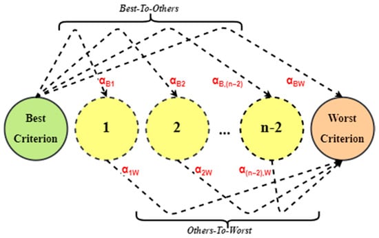
Figure 2.
How to perform reference comparisons in BWM.
- Step 1: The decision-making criteria are defined by the DM as .
- Step 2: The best and worst criteria are determined by DM.
- Step 3: Priorities of the best criterion over other criteria (BO) are determined by the DM as numbers between 1 and 9, which are written as .
- Step 4: Priorities of other criteria over the worst criterion (OW) are determined by the DM as numbers between 1 and 9, which are written as .
- Step 5: Calculating the weights of the criteria, ; the mathematical model of BWM is based on the BO and OW priority vectors.
Optimal weights of the criteria must satisfy the following equations: . To satisfy these conditions, a solution must be found that for each j, maximizes and .
Optimal weights of the criteria in BWM are obtained using Equation (1):
Calculating the CR in BWM: using obtained from Equation (1) and consistency index (CI) provided in Table 1, CR can be calculated as Equation (2) [26]:

Table 1.
Consistency index in BWM.
3.2. The SBWM
The proposed approach in this study calculates two weights for each of the criteria. The first weight is obtained using the best-to-others (BO) preference vector and the second weight is obtained using the others-to-worst (OW) preference vector. Then, the final weight is calculated as a combination of these two weights. One of the goals of the proposed approach is to achieve a powerful computational platform with easy-to-use capabilities that allows the weighing of quantitative and qualitative characteristics that affect the decision-making process.
The steps of SBWM are as follows:
- Step 1: The DM determines the set of criteria as and selects the best and worst criteria.
- Step 2: The priorities of the best criterion over the rest of the criteria (best-to-others) are determined by the DM as numbers between 1 and 9, which are displayed as the vector .
- Step 3: Similar to the previous step, the priorities of all criteria over the worst criterion (Others-to-Worst) are determined by the DM as numbers between 1 and 9, which are displayed as the vector .
- Step 4: Obtaining the weights of the decision criteria based on reference comparisons of the best criterion to the other criteria the equation of priority of BO is formed as Equation (3) and the best criterion weight is calculated. Then, the weights of the other criteria are obtained by substituting the best criterion weight in Equation (4).In another way, we can first calculate the initial weights for the criteria using the equation , then the criteria weights are calculated by normalizing the initial weights using the equation which will be equal to the weights obtained from Equations (3) and (4).
- Step 5: Obtaining the weights of the decision criteria based on reference comparisons of others-to-worst (: the OW priority equation is formed as Equation (5) and the worst criterion weight is calculated. Then, the weights of the other criteria are obtained by substituting the worst criterion weight in Equation (6).In another way, we can first calculate the initial weights for the criteria using the equation , then the criteria weights are calculated by normalizing the initial weights using the equation which will be equal to the weights obtained from Equations (5) and (6).
- Step 6: Obtaining the final weights of the decision criteria: the final weights of the criteria are calculated using a linear combination (Equation (7)). The value of the α parameter in Equation (7) represents the significance of the weights obtained in the two reference comparisons BO and OW and is determined by the DM as a number between 0 and 1.
Here, the researcher can decide which of the two weights will play a greater role in determining the final weights. Overall, α = 0.5 makes more sense. Setting α = 0.5 means that both the BO and OW vectors are equally important, assuming that the DM has answered all the questions of the questionnaire with sufficient accuracy. However, if there is an argument that the DM answers the initial questions of the questionnaire more carefully and that the DM’s accuracy and focus may be reduced when he makes comparisons, then we can choose a value greater than 0.5 for α and in this situation, the weights obtained from the BO vector are more important for determining the final weights.
3.2.1. Consistency Measurement in SBWM
Inconsistent pairwise comparisons lead to inaccurate calculations of priority vector and incorrect rankings of decision criteria and reduce the reliability of DM preferences. Measurement of consistency is used as an important tool to ensure that pairwise comparisons are logical. The consistency measurement mechanism presented in this study is different from the ratio provided in the original BWM. It is clear that if the DM pairwise comparisons are fully consistent, the weights obtained from BO and OW modes (Steps 4 and 5 of the proposed method) will be the same.
Otherwise, as the inconsistency increases, the difference between the weights calculated in these two modes increases. The recommended consistency rate (CR) in this study is calculated based on the sum of absolute differences of the weights calculated from BO and OW modes (Equation (8)). Given that the full consistency in DM pair comparisons is usually unattainable, the closer the CR is to zero, the more consistent the comparisons are.
Therefore, lower CR values are better. This index can also be divided by the number of criteria CR/n to determine differences between the weights obtained from the two comparison vectors. This is especially justified when a large number of criteria are compared.
If the obtained CR is greater than the acceptable DM threshold, it is necessary to revise the pairwise comparisons. Identifying which pairwise comparisons are inconsistent is an important challenge for the DM. For this purpose, a measure known as source of inconsistency (SI) is introduced and correcting related pairwise comparisons will lead to acceptable level of consistency. The SI index is also used to determine the source of inconsistency and it is used only when the CR has a large value; for example, when the CR value is increased, calculation of the SI index will show. When the CR value increases, the SI calculation will show which criterion comparisons made by the decision-maker are incorrect. Equation (9) can help the DM identify the SI.
3.2.2. Total Deviation (TD)
The TD index is used to measure the Euclidean distance between the weight ratios and , and pairwise comparisons related to them. The closer the weight ratio obtained by the model is to the DM preferences, the smaller the TD is [26]. TD can be calculated using Equation (10):
The smaller the TD value, the lower the error rate in decision-maker comparisons. Additionally, in order to have more appropriate values for TD, it can be divided by the number of criteria as TDBWM/2n, where n is the number of criteria [26].
3.3. Quantitative-Qualitative Method (QQM)
This section describes a method for evaluating life cycle of buildings criteria [12]. The proposed method considers the weighting of the criteria according to different qualitative and quantitative aspects simultaneously. A group decision matrix is formed to select the best building life cycle and perform an analysis of various project criteria. The life cycle of a project cannot be described on the mere basis of quantitative criteria, and there is a need for a system of simultaneous evaluation of quantitative and qualitative criteria. Such a variety of criteria requires a more specialized method of problem solving. In the project evaluation, the analysis of a set of economic, technical, qualitative, infrastructural, and other aspects should be considered that provide quantitative and qualitative descriptions of this information.
- Step 1: The sum of the values for each of the quantitative criteria is calculated from the following equation:where indicates the value assigned by the i criterion in the j alternative. In addition, t represents the number of quantitative criteria and n represents the number of problem options.
- Step 2: For each of the quantitative criteria, the problem of expressing the total monetary expression is calculated from the following equation:where the initial weight of the i criterion is denoted by .The quantitative criteria are divided into two categories according to their impact on projects: (a) short-term factors that have an impact on a particular period and (b) long-term factors that affect the entire life cycle of the project.The initial weight of short-term criteria such as construction cost is calculated as . For long-term costs such as maintenance costs, time needs to be taken into account, so the initial weight of long-term criteria can be calculated as ; where is the repayment time of the project and is the monetary evaluation of the i criterion.
- Step 3: The total value of the quantitative criteria is calculated from the following equation:
- Step 4: The weight of the quantitative criteria can be calculated using the following equation:where .
- Step 5: To match the weight of the quantitative and qualitative criteria, a standard value called is calculated. This value is equal to the sum of each selected importance of the quantitative criteria. In this case, the weighting of the qualitative criteria is calculated by comparing their usefulness with the standard value of . Equation (15) shows how is calculated:where indicates the quantitative standard weight of ; and indicates the number of quantitative criteria.
- Step 6: The initial weight of the qualitative criteria is expressed by the experts through comparing it with the standard value of as a percentage.
- Step 7: The equation to calculate the weight of the qualitative criteria as follows:
4. Numerical Examples
In this section, three simple numerical examples are provided to show the application and capabilities of the SBWM. The results of the SBWM are compared with the results of the original linear and nonlinear BWM and the TD level of the methods is analyzed and discussed.
4.1. Example 1
Assume that four criteria are available for evaluation and that the DM seeks to rank and weight these criteria. First, based on the reference comparisons in BWM, the priorities of the criteria are determined as numbers between 1 and 9. Table 2 shows the DM preferences.
Table 2.
DM preferences in Example 1.
To calculate the weights of the decision criteria using the BO priority vector, first, the best criterion weight is calculated from Equation (3). Then, the weights of other criteria are obtained by substituting the weight of the best criterion in Equation (4). Equation (17) calculates the best criterion weight and Equation (18) calculates the weights of the other criteria based on Step 4 of the proposed method.
Calculation of the weights of the decision criteria based on the OW priority vector is performed using Equations (5) and (6). Equation (19) calculates the worst criterion weight and Equation (20) calculates the weights of the other criteria based on Step 5 of the proposed method (calculating the weights based on OW priority vector).
After calculating the double weights of the criteria using BO and OW priority vectors, the final weights of the decision criteria can be calculated. These final weights are calculated using Equation (7). In Example 1, these weights are calculated using Equation (21) for α = 0.5. The α level determines the importance of the double weights in calculating the final weights of the criteria and its value is between 0 and 1.
In this study, comparative analysis was used as an approach to assess the validity and performance of the proposed method and compare it with BWM linear and nonlinear models. Table 3 shows the results of the proposed method for α = 0.5 and compares it with the results of BWM linear and nonlinear models. The TD index was also measured for all three methods, and the results showed that the proposed method had a lower TD than the other two methods.
Table 3.
Comparison of the results for Example 1.
Lower TD levels means that the obtained weights using the priority vectors selected by the DM are more consistent. Calculation of the value of the target function (denoted by ξ in the original BWM linear and nonlinear models) does not required in the proposed approach because there is no need to formulate a programming model.
Figure 3 compares the weights obtained by the proposed approach for α = 0.5 with the results of basic models of BWM for Example 1. The results suggest that the weights calculated by all three methods are very similar.
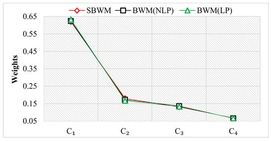
Figure 3.
Comparison of the weights calculated in Example 1.
Given that the proposed formula for calculating the inconsistency rate is specific to the proposed method and calculated based on the double weights obtained for each criterion, here this rate is calculated only for the proposed method. The CR is calculated using of Equation (8) and the sum of the absolute values of the differences of weights obtained in the two modes of BO and OW. In Example 1, this rate is calculated as follows:
4.2. Example 2
Suppose that the DM intends to rank and weigh five criteria. First, the priorities of the criteria over each other are determined based on the double priority vectors (as numbers between 1 and 9). Table 4 shows the priority vectors BO and OW for Example 2.
Table 4.
DM preferences in Example 2.
Equation (22) shows how to calculate the weight of the best criterion using the BO priority vector in Example 2; Equation (23) also shows how the weights of other criteria can be calculated using the weight of the best criterion.
Equation (24) shows the calculation of the worst criterion weight using the OW priority vector for Example 2, and Equation (25) calculate the weights of other decision criteria using the weight of the worst criterion.
Equation (26) shows the combination of the double weights obtained from the BO and OW priority vectors based on α = 0.5 for Example 2. These final weights are used for the final ranking of decision criteria.
In Table 5, the proposed method is compared with BWM linear and nonlinear models for α = 0.5. TD index also shows that in the nonlinear method, there is the least deviation between the calculated weights and the DM priority vectors. In general, however, the TD index in all three methods is not significantly different. In Example 2, the calculated value of CR of the proposed method using Equation (8) is 0.066 which indicates low inconsistency.
Table 5.
Comparison of the results in Example 2.
Figure 4 shows that the weights obtained using SBWM for α = 0.5 are very similar to the weights obtained using the other two models.
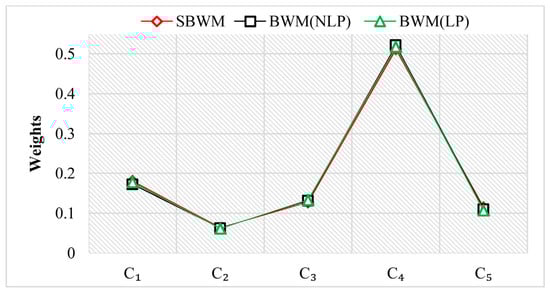
Figure 4.
Comparison of the weights calculated in Example 2.
4.3. Example 3
This example addresses the issue of decision-making regarding buildings’ energy efficiency barriers identified by [75]. In this study, energy efficiency barriers are divided into six main categories, and each category has several sub-criteria. Here, we consider only main barriers and ignore the sub-criteria.
The building sector has a great impact on the environment due to the use of natural resources, release of solid waste, creation of various forms of pollution, reduction of forests, and so on. In the entire life cycle of buildings, energy is consumed for the production of various components such as materials, steel, cement, brick, etc. during construction, the operation of the building, and destruction [75]. The reference comparisons made by the DM and the questionnaire are shown in Table 6. The six main barriers to energy efficiency in buildings are as follows:
Table 6.
Reference comparisons in Example 3.
- Economic Barriers (C1)
- Government Barriers (C2)
- Knowledge and Learning Barriers (C3)
- Market Related Barriers (C4)
- Organizational and Social Barriers (C5)
- Technological Barriers (C6)
Using the questionnaires completed by the DM and the reference comparisons, the best criterion weight is obtained using Equation (27). Then, by substituting the best criterion weight in Equation (28), the weights of the other elements of BO vector are obtained.
Then, using the reference comparisons between all the criteria and the worst criterion, the weight of the worst criterion is calculated using Equation (29) and by substituting this weight in Equation (30), other elements of OW weight vector are obtained.
Equation (7) is used to combine the weights of the BO and OW vectors, and the α level is assumed to be 0.5 by default. The final weights of the decision criteria as well as the comparisons between the proposed method and the BWM linear and nonlinear models are shown in Table 7. It is observed that the lowest amount of TD is obtained in the proposed method compared to the other two methods. Equation (31) shows how the final weights are calculated.
Table 7.
Comparison of the results in Example 3.
Table 7 shows that the proposed method has a lower TD value. The proposed approach and BWM linear and nonlinear models each create their own results, so different weights will be obtained from all three approaches. Figure 5, however, shows that what is more tangible than anything else is the closeness of the weights obtained from deferent methods and their uniform ranking. The CR of the proposed method is equal to 0.052, which indicates that comparisons made by the DM are consistent.
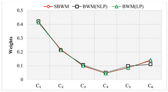
Figure 5.
Comparison of the weights calculated in Example 3.
5. Sensitivity Analysis
Sensitivity analysis is very important for designing new mathematical models and methodologies [76]. Sensitivity analysis was performed to evaluate the robustness of the final weights obtained using SBWM for different α values. After selecting the α value by the researcher in the range of 0 to 1, the TD (corresponding to the selected α value) is calculated to determine the lowest TD and the highest robustness of the obtained weights. Reducing the TD leads to increasing the robustness of the weights.
In BWM, the final weights of the decision criteria are calculated using the BO weight vector (which indicates the priorities of the best criterion over the other criteria) and the OW weight vector (which indicates the priorities of the other criteria over the worst criterion). In both vectors, the priorities of the criteria are determined by the DM as numbers between 1 and 9. The α parameter is introduced for combining the elements of both BO and OW vectors, which are obtained without the need for a programming model or mathematical software.
In the previous examples, the weights obtained from SBWM and the main BWM models were compared for α = 0.5. Selecting the value 0.5 for α by researcher indicates that both BO and OW weight vectors have equal importance, and the final weight of each criterion will be equally affected by both vectors.
However, as mentioned earlier, it may be argued that the DM (due to time constraints or fatigue) examines the questions at the beginning of the questionnaire more accurately (and makes more accurate comparisons for them). In such conditions, the researcher can select a number greater than 0.5 for α and give more importance to the BO weight vector. In this case, the final weight of each criterion will be more dependent on the BO weight vector and the OW weight vector will have fewer effects on the final results.
Table 8 shows the criteria weights obtained in all four examples for 0 ≤ α ≤ 1. For α = 0.5, both the BO and OW weight vectors have equal importance in calculating the final weight of each criterion. When α is changed, the final weight of each criterion is also changed. These changes are calculated and analyzed using the TD.
Table 8.
Sensitivity analysis of weights obtained by SBWM for 0 ≤ α ≤ 1 in 3 examples.
Figure 6 shows the weights obtained by SBWM, taking into account the α parameter in the range 0 to 1. Moreover, Figure 7 compares the TD for different values of α. When the DM preferences and comparisons are the most consistent with the final results of the computational approach or programming models, TD is minimized.
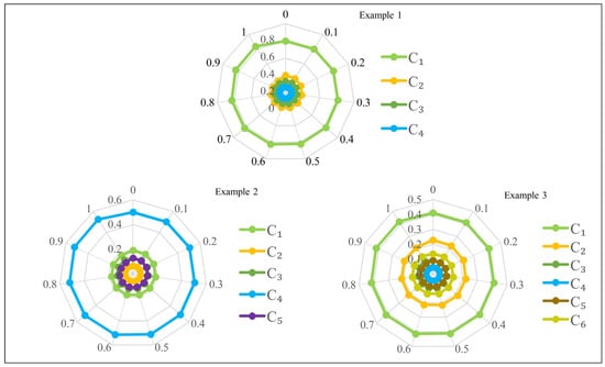
Figure 6.
Weights of decision criteria for 0 ≤ α ≤ 1 in sensitivity analysis.
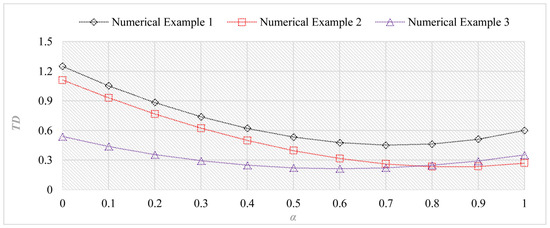
Figure 7.
Values of TD for 0 ≤ α ≤ 1 in sensitivity analysis.
The results of the sensitivity analysis showed that by changing the α level in the range of 0 to 1, the weights of different criteria change but the rankings do not change. In other words, changing the α level changes the importance of the criteria, but the final rankings of the criteria do not change, indicating that the results of the proposed method are robust.
Furthermore, if the rankings do not change when the α values change, it can be said that the pairwise comparisons made by the DMs and their preferences have a good consistency. On the other hand, lower values of TD (which shows the difference between the DM preferences and the weights obtained by the proposed model) indicate lower error and higher reliability of the results.
6. Determining the Importance of Buildings Life Cycle Assessment Criteria
This section describes the QQM [77]. The QQM is an MCDM technique introduced by Kaklauskas [77]. The QQM has been used to obtain criteria weights in decision-making in various fields [12,78,79,80]. The QQM is also known as a method of complex determination of the significances of the criteria taking into account their quantitative and qualitative characteristics. In this section, according to the data in [64], the weight of the buildings life cycle assessment criteria is calculated using QQM and SBWM, which are described in the methodology section. The combined weight of both methods is then calculated, and the results are analyzed. The decision-making problem in study [64] was to determine the weight of the buildings life cycle assessment criteria and finally to select the appropriate alternative according to the data and weights obtained from the QQM method.
Choosing the right criteria is a key step in making a decision. There are two ways to select criteria. One way is to review some articles and use them to select the appropriate criteria. Another way is to consult with experts and use the items they choose [81]. In this study, the importance of decision criteria using QQM and SBWM and the combination of weights obtained from both methods are discussed. The required data, including decision criteria, measure, and decision matrix, are shown in Table 9; for more information on how to select indicators and theoretical concepts, you can refer to the study.
Table 9.
The results of a complex determination of the weights using QQM.
The data needed to decide on the life cycle assessment indicators of the buildings were collected using a questionnaire distributed among 35 experts who were asked to express their preferences regarding the 14 selected criteria. A number of respondents were selected from among members of several organizations (including owners, designers, contractors, and scientists). The remaining respondents were real estate appraisers, brokers, and other specialists. The values of the quantitative criteria were determined based on the analyzed projects, price lists, specifications, reference books, and recommendations [80]. A more complete description of the data presented in Table 9 is available in reference [82].
Using Equations (11)–(16) in the QQM method, the weight of quantitative and qualitative criteria was obtained. As it can be seen, DC1 and DC2 are quantitative criteria, and DC3 to DC14 are qualitative. Having passed special steps to gain the importance of decision criteria, we have tabulated the final weight of each of the 14 criteria in the weight column in Table 9.
In order to obtain the importance of the buildings life cycle assessment criteria using SBWM and compare and combine the results with QQM, two separate pairwise comparisons were performed. Once the quantitative criteria were measured by the experts, and once again the qualitative criteria were analyzed and evaluated. The expert panel consisted of five experts from the construction industry who decided to agree on preferences over other criteria. Thus, for each of the quantitative and qualitative criteria, pairwise comparisons were made only once, and the results were obtained using the SBWM described in the methodology section.
If the experts had not agreed on their preferences, each expert would have had to make a pairwise comparison for each of the quantitative and qualitative criteria separately, and finally a combination of the final weights obtained from each expert would have been presented. From among the quantitative criteria, DC1 was selected as the most important criterion and DC2 as the least important criterion.
The BO and OW preference vectors are formed in order to obtain the final weight of the quantitative criteria using the experts’ preferences, and the pairwise comparisons and preferences are shown in Table 10. Furthermore, DC4 and DC11 are mentioned as the most important and least important qualitative criteria by the experts respectively, Also, the pairwise comparisons and experts’ preferences regarding qualitative criteria are shown in Table 10.
Table 10.
Experts’ preferences regarding quantitative and qualitative criteria.
Using SBWM, the final weight of the quantitative and qualitative indicators was calculated, and the final results of the QQM and SBWM methods and the combination of the weights of both methods are shown and analyzed in Table 11.
Table 11.
Numerical value of weights obtained from the proposed methods.
Based on the final weight obtained from both methods, DC1 = 0.840 has the highest weight among the quantitative indices. Among the qualitative criteria, DC4 = 0.234, DC6 = 0.147 and DC3 = 0.111 are the most important among other qualitative criteria respectively. Figure 8 shows the final weights obtained from the QQM and SBWM methods and the weight combinations of both methods on the quantitative criteria. In addition, in Figure 9, the obtained weights of qualitative criteria of the proposed approach are compared.
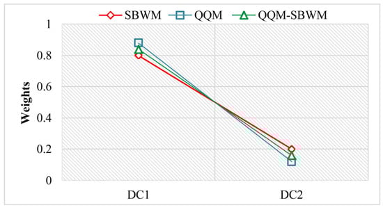
Figure 8.
The weights obtained for quantitative criteria.
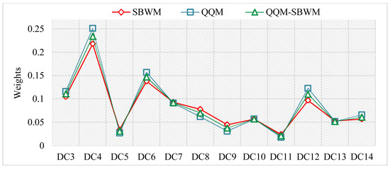
Figure 9.
The weights obtained for qualitative criteria.
With regard to the advancement of technology in the world and the size of existing infrastructure, it is necessary to use evaluation systems that are compatible with new conditions and can be used in all stages of construction and production [83]. Assessing the life cycle of buildings and the results of studies published on this area includes several benefits for stakeholders in the construction industry. For example, governments can benefit from the results of this study to review and build new buildings using new technologies in the construction market [84]. Moreover, construction companies can use the results of this study in product or service development, market development, or supplier and participant selection [85]. Finally, researchers can use these results to address the challenges of building construction [86]. The results of the development of the proposed approach in this study show that combining QQM with SBWM and applying this combination to various decision-making issues can help managers and experts as a powerful decision support tool. This can be concluded considering the advantages of QQM, such as the possibility of determining the weight of the quantitative and qualitative criteria simultaneously in different decision-making issues, as well as the possibility of assessing the degree of participants’ satisfaction in various projects and checking their needs.
In addition, the advantages of the SBWM method—such as simple calculations, not requiring a computer-based platform to solve the problem, and reducing the computational complexity of the problem—are also effective in this regard. Using a decision support system (DSS) provides a more practical approach for construction industry participants [80] and enables decision-makers to make the most of the capabilities of the proposed approach.
The results of simplified BWM were evaluated in three numerical examples and the values of TD and CR were calculated. In each example, the results were compared with the results obtained from the basic BWM separately. In some cases, the TD values of the proposed method were improved compared to the basic BWM. By performing the sensitivity analysis, the final weights were also calculated for different values of the α parameter and the results showed that the final weights had high robustness and reliability. In the practical application of the research, we evaluated the life cycle of buildings using a combination of SBWM and QQM methods and the weights obtained from both methods were combined. We use a simple average method to combine the weights of the two methods. We can use a weighted average as well, but we prefer that both methods contribute equally to the final results. The outputs of both SBWM and QQM are the weights of the decision criteria that have the same dimension; therefore, the final weights can be calculated by combining the weights using the simple average method. Qualitative and quantitative methods each have strengths and weaknesses that limit their use. The QQM-SBWM hybrid method seeks to combine these two approaches and create a new model to take advantage of both methods. The hybrid QQM-SBWM method can be a new and appropriate approach to solve various decision-making problems in many areas.
7. Conclusions
In this paper, a new combined approach based on the computational model of BWM (called SBWM) and QQM was proposed to evaluate buildings’ life cycle and determine the weights of decision criteria. Life cycle analysis of buildings can have very beneficial results for environmental care and, ultimately, sustainability. This analysis usually examines the effects of the building in terms of pollution, greenhouse gas emissions, water consumption, energy consumption, material consumption, and other factors on the environment. Some of these effects may be local, and some may be manifested through diffusion into the air and surface and groundwater regionally or even globally. Therefore, evaluating the life cycle of buildings is an important and necessary issue for decision-makers and policy-makers in the field of construction.
In the SBWM method, the basic idea of the original BWM in relation to reference comparisons is still used but the calculations become simpler and there is no need to solve the linear and nonlinear programming model. The ability to solve the model without using a software platform is another advantage of the proposed method. In recent years, the use of BWM has become very popular; however, in all studies, the weights of the criteria have been obtained by solving linear or nonlinear models. On the other hand, in previous studies, quantitative and qualitative criteria have not been separated; separating these criteria and then calculating their weights using QQM can provide more accurate results. Using the SBWM model eliminates the need for special software packages. In addition, this method will still be applicable when the number of dimensions is very large, while in the conventional method for determining the weights of criteria using BWM, the complexity of the problem is increased by increasing the dimensions of the problem. The QQM has the ability to obtain the weights of quantitative and qualitative criteria simultaneously; therefore, providing a combined approach based on the QQM and SBWM methods can be an effective approach to solving decision-making problems. SBWM first calculates the weights of the criteria based on two priority vectors of BWM, and then calculates the final weights of the criteria. To evaluate the validity and applicability of the proposed method, the method was compared with BWM linear and nonlinear models. These comparisons were made in the form of three numerical examples and one real example adapted from other studies. The proposed model showed that it could provide results close to the BWM linear and nonlinear models. In general, there was not much difference between the weights obtained from LP, NLP, and SBWM models. In addition, the TD level of the proposed method was often close or less than the other two methods. The results of the proposed method showed that it is possible to reach a solution space based on BWM reference comparisons, which is very close to an optimal solution. It has also been shown that if DM preferences are consistent, changing the α level will not change the ranking of criteria and the results of the proposed method are robust. The results of the proposed hybrid approach showed that among the quantitative and qualitative criteria, estimated cost, comfort level, and basic floor area are, in order, the most important among other criteria. Decision-makers in the field of construction and policy-makers in this field can use the results of this research on issues related to the life cycle of buildings.
There are several suggestions for future research. Combining the proposed approach with other existing MCDM methods can be investigated in future research. Similarly, expanding the proposed approach to group decision-making can be attractive. Furthermore, in this study, DM preferences have been considered definitively; in future research, it is possible to consider uncertainty in DM preferences to bring the issue closer to the real world. The development of SBWM using rough theory for group decision-making can also be interesting; this approach can also be compared with other criteria weighting methods such as AHP, SWARA (stepwise weight assessment ratio analysis), LINMAP (linear programming technique for multidimensional analysis of preference), and MEREC (MEthod based on the Removal Effects of Criteria).
Author Contributions
Conceptualization, M.A.; methodology, M.H.-T. and E.K.Z. and M.G.; validation, M.K.-G. and A.K.; formal analysis, M.A. and M.H.-T.; investigation, E.K.Z. and M.G.; resources, E.K.Z. and A.K.; data curation, M.K.-G. and M.A.; writing—original draft preparation, M.H.-T. and M.G.; writing—review and editing, M.A. and E.K.Z.; supervision, M.K.-G. and A.K. All authors have read and agreed to the published version of the manuscript.
Funding
There is no external fund for this study.
Institutional Review Board Statement
Not applicable.
Informed Consent Statement
Not applicable.
Data Availability Statement
Not applicable.
Conflicts of Interest
The authors declare no conflict of interest.
References
- International Organization for Standardization. Environmental Management: Life Cycle Assessment; Principles and Framework; ISO: Geneva, Switzerland, 2006; Volume 14044, ISBN 0626183502. [Google Scholar]
- Bilec, M.; Ries, R.; Matthews, H.S.; Sharrard, A.L. Example of a hybrid life-cycle assessment of construction processes. J. Infrastruct. Syst. 2006, 12, 207–215. [Google Scholar] [CrossRef]
- Hollberg, A.; Ruth, J. LCA in architectural design—A parametric approach. Int. J. Life Cycle Assess. 2016, 21, 943–960. [Google Scholar] [CrossRef]
- Nwodo, M.N.; Anumba, C.J. A review of life cycle assessment of buildings using a systematic approach. Build. Environ. 2019, 162, 106290. [Google Scholar] [CrossRef]
- Xue, Z.; Liu, H.; Zhang, Q.; Wang, J.; Fan, J.; Zhou, X. The Impact Assessment of Campus Buildings Based on a Life Cycle Assessment–Life Cycle Cost Integrated Model. Sustainability 2020, 12, 294. [Google Scholar] [CrossRef]
- Chau, C.K.; Leung, T.M.; Ng, W.Y. A review on life cycle assessment, life cycle energy assessment and life cycle carbon emissions assessment on buildings. Appl. Energy 2015, 143, 395–413. [Google Scholar] [CrossRef]
- Dong, Y.H.; Ng, S.T. A life cycle assessment model for evaluating the environmental impacts of building construction in Hong Kong. Build. Environ. 2015, 89, 183–191. [Google Scholar] [CrossRef]
- Alizadeh, R.; Beiragh, R.G.; Soltanisehat, L.; Soltanzadeh, E.; Lund, P.D. Performance evaluation of complex electricity generation systems: A dynamic network-based data envelopment analysis approach. Energy Econ. 2020, 91, 104894. [Google Scholar] [CrossRef]
- Williams, J.; Alizadeh, R.; Allen, J.K.; Mistree, F. Using Network Partitioning to Design a Green Supply Chain. In Proceedings of the International Design Engineering Technical Conferences and Computers and Information in Engineering Conference; American Society of Mechanical Engineers: New York, NY, USA, 2020; Volume 84010, p. V11BT11A050. [Google Scholar]
- Zabalza, I.; Scarpellini, S.; Aranda, A.; Llera, E.; Jáñez, A. Use of LCA as a tool for building ecodesign. A case study of a low energy building in Spain. Energies 2013, 6, 3901–3921. [Google Scholar] [CrossRef]
- Kofoworola, O.F.; Gheewala, S.H. Environmental life cycle assessment of a commercial office building in Thailand. Int. J. Life Cycle Assess. 2008, 13, 498–511. [Google Scholar] [CrossRef]
- Zavadskas, E.K.; Kaklauskas, A.; Kvederytė, N. Multivariant design and multiple criteria analysis of a building life cycle. Informatica 2001, 12, 169–188. [Google Scholar]
- Brooks, R.J.; Tobias, A.M. Choosing the best model: Level of detail, complexity, and model performance. Math. Comput. Model. 1996, 24, 1–14. [Google Scholar] [CrossRef]
- Tzeng, G.-H.; Huang, J.-J. Multiple Attribute Decision Making: Methods and Applications; Chapman and Hall/CRC: Boca Raton, FL, USA, 2011; ISBN 0429110707. [Google Scholar]
- Zhang, H.; Kou, G.; Peng, Y. Soft consensus cost models for group decision making and economic interpretations. Eur. J. Oper. Res. 2019, 277, 964–980. [Google Scholar] [CrossRef]
- Kou, G.; Lin, C. A cosine maximization method for the priority vector derivation in AHP. Eur. J. Oper. Res. 2014, 235, 225–232. [Google Scholar] [CrossRef]
- Wang, J.-J.; Jing, Y.-Y.; Zhang, C.-F.; Zhao, J.-H. Review on multi-criteria decision analysis aid in sustainable energy decision-making. Renew. Sustain. Energy Rev. 2009, 13, 2263–2278. [Google Scholar] [CrossRef]
- Kumar, A.; Sah, B.; Singh, A.R.; Deng, Y.; He, X.; Kumar, P.; Bansal, R.C. A review of multi criteria decision making (MCDM) towards sustainable renewable energy development. Renew. Sustain. Energy Rev. 2017, 69, 596–609. [Google Scholar] [CrossRef]
- Baumann, M.; Weil, M.; Peters, J.F.; Chibeles-Martins, N.; Moniz, A.B. A review of multi-criteria decision making approaches for evaluating energy storage systems for grid applications. Renew. Sustain. Energy Rev. 2019, 107, 516–534. [Google Scholar] [CrossRef]
- Kabir, G.; Sadiq, R.; Tesfamariam, S. A review of multi-criteria decision-making methods for infrastructure management. Struct. Infrastruct. Eng. 2014, 10, 1176–1210. [Google Scholar] [CrossRef]
- Alizadeh, R.; Lund, P.D.; Soltanisehat, L. Outlook on biofuels in future studies: A systematic literature review. Renew. Sustain. Energy Rev. 2020, 134, 110326. [Google Scholar] [CrossRef]
- Guarini, M.R.; Battisti, F.; Chiovitti, A. A methodology for the selection of multi-criteria decision analysis methods in real estate and land management processes. Sustainability 2018, 10, 507. [Google Scholar] [CrossRef]
- Campos-Guzmán, V.; García-Cáscales, M.S.; Espinosa, N.; Urbina, A. Life Cycle Analysis with Multi-Criteria Decision Making: A review of approaches for the sustainability evaluation of renewable energy technologies. Renew. Sustain. Energy Rev. 2019, 104, 343–366. [Google Scholar] [CrossRef]
- Alizadeh, R.; Soltanisehat, L.; Lund, P.D.; Zamanisabzi, H. Improving renewable energy policy planning and decision-making through a hybrid MCDM method. Energy Policy 2020, 137, 111174. [Google Scholar] [CrossRef]
- Chumaidiyah, E.; Dewantoro, M.D.R.; Kamil, A.A. Design of a Participatory Web-Based Geographic Information System for Determining Industrial Zones. Appl. Comput. Intell. Soft Comput. 2021, 2021, 6665959. [Google Scholar] [CrossRef]
- Rezaei, J. Best-worst multi-criteria decision-making method. Omega 2015, 53, 49–57. [Google Scholar] [CrossRef]
- Mi, X.; Tang, M.; Liao, H.; Shen, W.; Lev, B. The state-of-the-art survey on integrations and applications of the best worst method in decision making: Why, what, what for and what’s next? Omega 2019. [Google Scholar] [CrossRef]
- Amiri, M.; Tabatabaei, M.H.; Ghahremanloo, M.; Keshavarz-Ghorabaee, M.; Zavadskas, E.K.; Antucheviciene, J. A new fuzzy approach based on BWM and fuzzy preference programming for hospital performance evaluation: A case study. Appl. Soft Comput. 2020, 106279. [Google Scholar] [CrossRef]
- Jia, L.; Alizadeh, R.; Hao, J.; Wang, G.; Allen, J.K.; Mistree, F. A rule-based method for automated surrogate model selection. Adv. Eng. Inform. 2020, 45, 101123. [Google Scholar] [CrossRef]
- Bai, C.; Kusi-Sarpong, S.; Badri Ahmadi, H.; Sarkis, J. Social sustainable supplier evaluation and selection: A group decision-support approach. Int. J. Prod. Res. 2019, 7046–7067. [Google Scholar] [CrossRef]
- Gupta, H.; Barua, M.K. Supplier selection among SMEs on the basis of their green innovation ability using BWM and fuzzy TOPSIS. J. Clean. Prod. 2017, 152, 242–258. [Google Scholar] [CrossRef]
- Haeri, S.A.S.; Rezaei, J. A grey-based green supplier selection model for uncertain environments. J. Clean. Prod. 2019, 221, 768–784. [Google Scholar] [CrossRef]
- Jafarzadeh Ghoushchi, S.; Khazaeili, M.; Amini, A.; Osgooei, E. Multi-criteria sustainable supplier selection using piecewise linear value function and fuzzy best-worst method. J. Intell. Fuzzy Syst. 2019, 37, 2309–2325. [Google Scholar] [CrossRef]
- Vahidi, F.; Torabi, S.A.; Ramezankhani, M.J. Sustainable supplier selection and order allocation under operational and disruption risks. J. Clean. Prod. 2018, 174, 1351–1365. [Google Scholar] [CrossRef]
- Amiri, M.; Hashemi-Tabatabaei, M.; Ghahremanloo, M.; Keshavarz-Ghorabaee, M.; Zavadskas, E.K.; Banaitis, A. A new fuzzy BWM approach for evaluating and selecting a sustainable supplier in supply chain management. Int. J. Sustain. Dev. World Ecol. 2020. [Google Scholar] [CrossRef]
- You, P.; Guo, S.; Zhao, H.; Zhao, H. Operation performance evaluation of power grid enterprise using a hybrid BWM-TOPSIS method. Sustainability 2017, 9, 2329. [Google Scholar] [CrossRef]
- Zhao, H.; Guo, S.; Zhao, H. Comprehensive performance assessment on various battery energy storage systems. Energies 2018, 11, 2841. [Google Scholar] [CrossRef]
- Zhao, H.; Zhao, H.; Guo, S. Comprehensive Performance Evaluation of Electricity Grid Corporations Employing a Novel MCDM Model. Sustainability 2018, 10, 2130. [Google Scholar] [CrossRef]
- Kumar, A.; Aswin, A.; Gupta, H. Evaluating green performance of the airports using hybrid BWM and VIKOR methodology. Tour. Manag. 2020, 76, 103941. [Google Scholar] [CrossRef]
- Chen, Z.; Ming, X.; Zhou, T.; Chang, Y.; Sun, Z. A hybrid framework integrating rough-fuzzy best-worst method to identify and evaluate user activity-oriented service requirement for smart product service system. J. Clean. Prod. 2020, 253, 119954. [Google Scholar] [CrossRef]
- Hussain, A.; Chun, J.; Khan, M. A novel framework towards viable Cloud Service Selection as a Service (CSSaaS) under a fuzzy environment. Future Gener. Comput. Syst. 2020, 104, 74–91. [Google Scholar] [CrossRef]
- Keshavarz-Ghorabaee, M.; Amiri, M.; Hashemi-Tabatabaei, M.; Ghahremanloo, M. Prioritizing the Barriers and Challenges of Big Data Analytics in Logistics and Supply Chain Management Using MCDM. In Big Data Analytics in Supply Chain Management: Theory and Applications; CRC Press: Boca Raton, FL, USA, 2020; p. 29. [Google Scholar]
- Karimi, H.; Sadeghi-Dastaki, M.; Javan, M. A fully fuzzy best–worst multi attribute decision making method with triangular fuzzy number: A case study of maintenance assessment in the hospitals. Appl. Soft Comput. J. 2020, 86, 105882. [Google Scholar] [CrossRef]
- Maghsoodi, A.I.; Rasoulipanah, H.; López, L.M.; Liao, H.; Zavadskas, E.K. Integrating Interval-valued Multi-granular 2-tuple Linguistic BWM-CODAS Approach with Target-based Attributes: Site Selection for a Construction Project. Comput. Ind. Eng. 2019, 139, 106147. [Google Scholar] [CrossRef]
- Rahimi, S.; Hafezalkotob, A.; Monavari, S.M.; Hafezalkotob, A.; Rahimi, R. Sustainable landfill site selection for municipal solid waste based on a hybrid decision-making approach: Fuzzy group BWM-MULTIMOORA-GIS. J. Clean. Prod. 2020, 248, 119186. [Google Scholar] [CrossRef]
- Tabatabaei, M.H.; Firouzabadi, S.M.A.K.; Amiri, M.; Ghahremanloo, M. A combination of the fuzzy best-worst and Vikor methods for prioritisation the Lean Six Sigma improvement projects. Int. J. Bus. Contin. Risk Manag. 2020, 10, 267–277. [Google Scholar] [CrossRef]
- Zhou, J.; Wu, Y.; Wu, C.; He, F.; Zhang, B.; Liu, F. A geographical information system based multi-criteria decision-making approach for location analysis and evaluation of urban photovoltaic charging station: A case study in Beijing. Energy Convers. Manag. 2020, 205, 112340. [Google Scholar] [CrossRef]
- Liu, A.; Zhao, Y.; Meng, X.; Zhang, Y. A three-phase fuzzy multi-criteria decision model for the charging station location of the sharing electric vehicle. Int. J. Prod. Econ. 2019, 225, 107572. [Google Scholar] [CrossRef]
- Ghoushchi, S.J.; Yousefi, S.; Khazaeili, M. An extended FMEA approach based on the Z-MOORA and fuzzy BWM for prioritization of failures. Appl. Soft Comput. 2019, 81, 105505. [Google Scholar] [CrossRef]
- Luo, S.; Xing, L. A Hybrid Decision Making Framework for Personnel Selection Using BWM, MABAC and PROMETHEE. Int. J. Fuzzy Syst. 2019, 21, 2421–2434. [Google Scholar] [CrossRef]
- Pamucar, D.; Chatterjee, K.; Zavadskas, E.K. Assessment of third-party logistics provider using multi-criteria decision-making approach based on interval rough numbers. Comput. Ind. Eng. 2019, 127, 383–407. [Google Scholar] [CrossRef]
- Ramezanali, A.K.; Feizi, F.; Jafarirad, A.; Lotfi, M. Application of Best-Worst method and Additive Ratio Assessment in mineral prospectivity mapping: A case study of vein-type copper mineralization in the Kuhsiah-e-Urmak Area, Iran. Ore Geol. Rev. 2020, 117, 103268. [Google Scholar] [CrossRef]
- van de Kaa, G.; Fens, T.; Rezaei, J. Residential grid storage technology battles: A multi-criteria analysis using BWM. Technol. Anal. Strateg. Manag. 2019, 31, 40–52. [Google Scholar] [CrossRef]
- Rezaei, J. Best-worst multi-criteria decision-making method: Some properties and a linear model. Omega 2016, 64, 126–130. [Google Scholar] [CrossRef]
- Guo, S.; Zhao, H. Fuzzy best-worst multi-criteria decision-making method and its applications. Knowl. Based Syst. 2017, 121, 23–31. [Google Scholar] [CrossRef]
- Mou, Q.; Xu, Z.; Liao, H. A graph based group decision making approach with intuitionistic fuzzy preference relations. Comput. Ind. Eng. 2017, 110, 138–150. [Google Scholar] [CrossRef]
- Pamučar, D.; Petrović, I.; Ćirović, G. Modification of the Best–Worst and MABAC methods: A novel approach based on interval-valued fuzzy-rough numbers. Expert Syst. Appl. 2018, 91, 89–106. [Google Scholar] [CrossRef]
- Aboutorab, H.; Saberi, M.; Asadabadi, M.R.; Hussain, O.; Chang, E. ZBWM: The Z-number extension of Best Worst Method and its application for supplier development. Expert Syst. Appl. 2018, 107, 115–125. [Google Scholar] [CrossRef]
- Li, J.; Wang, J.; Hu, J. Multi-criteria decision-making method based on dominance degree and BWM with probabilistic hesitant fuzzy information. Int. J. Mach. Learn. Cybern. 2019, 10, 1671–1685. [Google Scholar] [CrossRef]
- Hafezalkotob, A.; Hafezalkotob, A. A novel approach for combination of individual and group decisions based on fuzzy best-worst method. Appl. Soft Comput. J. 2017, 59, 316–325. [Google Scholar] [CrossRef]
- Safarzadeh, S.; Khansefid, S.; Rasti-Barzoki, M. A group multi-criteria decision-making based on best-worst method. Comput. Ind. Eng. 2018, 126, 111–121. [Google Scholar] [CrossRef]
- Mohammadi, M.; Rezaei, J. Bayesian best-worst method: A probabilistic group decision making model. Omega 2019. [Google Scholar] [CrossRef]
- Tabatabaei, M.H.; Amiri, M.; Khatami Firouzabadi, S.M.A.; Ghahremanloo, M.; Keshavarz-Ghorabaee, M.; Saparauskas, J. A new group decision-making model based on bwm and its application to managerial problems. Transform. Bus. Econ. 2019, 18, 197–214. [Google Scholar]
- Tabatabaei, M.H.; Amiri, M.; Ghahremanloo, M.; Keshavarz-Ghorabaee, M.; Zavadskas, E.K.; Antucheviciene, J. Hierarchical Decision-making using a New Mathematical Model based on the Best-worst Method. Int. J. Comput. Commun. Control 2019, 14, 710–725. [Google Scholar] [CrossRef]
- Liao, H.; Mi, X.; Yu, Q.; Luo, L. Hospital performance evaluation by a hesitant fuzzy linguistic best worst method with inconsistency repairing. J. Clean. Prod. 2019, 232, 657–671. [Google Scholar] [CrossRef]
- Ijadi Maghsoodi, A.; Mosavat, M.; Hafezalkotob, A.; Hafezalkotob, A. Hybrid hierarchical fuzzy group decision-making based on information axioms and BWM: Prototype design selection. Comput. Ind. Eng. 2019, 127, 788–804. [Google Scholar] [CrossRef]
- Brunelli, M.; Rezaei, J. A multiplicative best–worst method for multi-criteria decision making. Oper. Res. Lett. 2019, 47, 12–15. [Google Scholar] [CrossRef]
- Wu, Q.; Zhou, L.; Chen, Y.; Chen, H. An integrated approach to green supplier selection based on the interval type-2 fuzzy best-worst and extended VIKOR methods. Inf. Sci. 2019, 502, 394–417. [Google Scholar] [CrossRef]
- Mou, Q.; Xu, Z.; Liao, H. An intuitionistic fuzzy multiplicative best-worst method for multi-criteria group decision making. Inf. Sci. 2016, 374, 224–239. [Google Scholar] [CrossRef]
- Akbarian-Saravi, N.; Mobini, M.; Rabbani, M. Development of a comprehensive decision support tool for strategic and tactical planning of a sustainable bioethanol supply chain: Real case study, discussions and policy implications. J. Clean. Prod. 2020, 244, 118871. [Google Scholar] [CrossRef]
- Ali, A.; Rashid, T. Hesitant fuzzy best-worst multi-criteria decision-making method and its applications. Int. J. Intell. Syst. 2019, 34, 1953–1967. [Google Scholar] [CrossRef]
- Bonyani, A.; Alimohammadlou, M. A novel approach to solve the problems with network structure. Oper. Res. 2019, 1–19. [Google Scholar] [CrossRef]
- Amiri, M.; Emamat, M.S.M.M. A Goal Programming Model for BWM. Informatica 2020, 31, 21–34. [Google Scholar] [CrossRef]
- Amiri, M.; Hashemi-Tabatabaei, M.; Ghahremanloo, M.; Keshavarz-Ghorabaee, M.; Kazimieras Zavadskas, E.; Antucheviciene, J. A novel model for multi-criteria assessment based on BWM and possibilistic chance-constrained programming. Comput. Ind. Eng. 2021, 107287. [Google Scholar] [CrossRef]
- Gupta, P.; Anand, S.; Gupta, H. Developing a roadmap to overcome barriers to energy efficiency in buildings using best worst method. Sustain. Cities Soc. 2017, 31, 244–259. [Google Scholar] [CrossRef]
- Keshavarz-Ghorabaee, M.; Amiri, M.; Zavadskas, E.K.; Turskis, Z.; Antucheviciene, J. Determination of Objective Weights Using a New Method Based on the Removal Effects of Criteria (MEREC). Symmetry 2021, 13, 525. [Google Scholar] [CrossRef]
- Kaklauskas, A. Multiple Criteria Decision Support of Building Life Cycle; Vilnius Technika: Vilnius, Lithuania, 1999. [Google Scholar]
- Zavadskas, E.K.; Kaklauskas, A.; Banaitis, A.; Kvederyte, N. Housing credit access model: The case for Lithuania. Eur. J. Oper. Res. 2004, 155, 335–352. [Google Scholar] [CrossRef]
- Zavadskas, E.K.; Kaklauskas, A.; Vilutiene, T. Multicriteria evaluation of apartment blocks maintenance contractors: Lithuanian case study. Int. J. Strateg. Prop. Manag. 2009, 13, 319–338. [Google Scholar] [CrossRef]
- Banaitiene, N.; Banaitis, A.; Kaklauskas, A.; Zavadskas, E.K. Evaluating the life cycle of a building: A multivariant and multiple criteria approach. Omega 2008, 36, 429–441. [Google Scholar] [CrossRef]
- Bazrafshan, R.; Hashemkhani Zolfani, S.; Al-e-hashem, S.M.J. Comparison of the Sub-Tour Elimination Methods for the Asymmetric Traveling Salesman Problem Applying the SECA Method. Axioms 2021, 10, 19. [Google Scholar] [CrossRef]
- Kvederyte, N. Efficiency of Single-Family Houses in Harmonisation of Interests of Participants of Their Life Cycle. Ph.D. Thesis, Vilnius Gediminas Technical University, Vilnius, Lithuania, 2000. [Google Scholar]
- Shen, C.; Zhao, K.; Ge, J. An Overview of the Green Building Performance Database. J. Eng. 2020, 2020, 3780595. [Google Scholar] [CrossRef]
- Simonen, K. Life Cycle Assessment; Routledge: Oxfordshire, UK, 2014; ISBN 1317697367. [Google Scholar]
- Hauschild, M.Z.; Rosenbaum, R.K.; Olsen, S.I. Life Cycle Assessment; Springer: Berlin/Heidelberg, Germany, 2018; Volume 2018. [Google Scholar]
- Liu, H.; He, Y.; Hu, Q.; Guo, J.; Luo, L. Risk management system and intelligent decision-making for prefabricated building project under deep learning modified teaching-learning-based optimization. PLoS ONE 2020, 15, e0235980. [Google Scholar] [CrossRef] [PubMed]
Publisher’s Note: MDPI stays neutral with regard to jurisdictional claims in published maps and institutional affiliations. |
© 2021 by the authors. Licensee MDPI, Basel, Switzerland. This article is an open access article distributed under the terms and conditions of the Creative Commons Attribution (CC BY) license (https://creativecommons.org/licenses/by/4.0/).