1. Introduction
The global food crisis in 2008 had a significant and historical impact. It was reported that 963 million people suffered from hunger, and food crises occurred in poor and developing countries [
1]. World food prices continued to increase for almost all commodities during the 2007–2008 crisis, and prices jumped up sharply, and now the level of price volatility is getting higher. Global food security is one of the leading development priorities of every country, notably countries facing the threat of environmental changes [
2]. It also causes a reduction in the level of food availability, while populations requiring access to food continue to increase [
3]. Market instability from international agricultural products also makes it difficult to access food supplies [
4,
5]. In the concept of sustainable development, it is necessary to integrate environmental systems into economic and social policies [
6], including developing the community’s ability to access food. Food security development must not compromise the ability of future generations to meet their needs. The volatility of food prices during the global crisis caused food uncertainty to increase [
7,
8]. The most significant impact is felt by poor people in developing countries, whose food reserves depend on imports [
9].
Population growth is always increasing and causing a growing need for more food [
10]. If the agricultural food production capacity reaches the environmental limit, it is feared that food production and ecological conditions will be harmed [
11]. Food security can be achieved if the entire population has daily access to food with adequate nutrition. Changes in the level of prosperity will also shift the need for food nutrition that must be used to maintain food security [
12]. The Food and Agriculture Organization of the United Nations (FAO) in 2019 stated that globally, one in nine people experience hunger or difficulty accessing food with proper nutrition. Increasing food production is conventionally carried out by growing more in the agricultural areas, which means that it becomes a threat to biodiversity [
13]. The food system is the sector that contributes the most to greenhouse gas emissions. Due to the addition of agricultural land for food by employing deforestation and the food production process, which involves a distribution process that requires energy and chemicals to suppress crop pests [
14], FAO provided recommendations to all countries in the world to support the realization of sustainable food by carrying out efficiency in the food system, especially in the production process, creating policies to reduce consumption rates, and managing the system’s social economy while still referring to natural sustainability [
15].
Sustainable food refers to the growth of food supply based on environmental sustainability [
16]. Currently, a lot of food production has reached its limits and exceeds environmental capacity. Nitrogen synthesis and phosphorus use that have passed threshold levels, land-use changes, and human dependence on fossil energy contribute to increased greenhouse gas emissions. Food production from agriculture is also a driver of biodiversity loss [
13]. The global food system contributes to greenhouse gas emissions from agri-food production, processing, and distribution to retail and food preparation for households [
17]. In addition, the increase in food industrialization also has a broad impact on the environment. Policymakers are increasingly aware of the need to resolve food system problems. At the same time, they are also faced with an increased burden of food security, specifically in terms of nutrition and its relationship to global population growth. Sustainable food tries to solve two problems: how to support both a sustainable environment and the food system [
18].
Price volatility is one of the signals in detecting market instability, which can impact people’s welfare. Many studies have analyzed this issue, but only focused on price volatility, including future volatility and past trends, oil price volatility, export concentration, stock levels, and yields [
19]. Climate change is said to also have a significant impact on food security [
20,
21]. Financial securities and market fluctuations are also affected by extreme weather frequency, which psychologically influences investor behavior in making decisions, including food investment [
22,
23].
This study explicitly analyzes the influence of climate on food price volatility for a sustainable food system. Volatility is a value that shows how much and how fast something changes over time, such as what happens in commodity prices [
24]. Variations in food commodity prices can be a problem and increase the risk for actors in the food system: producers, consumers, and the government. In simple terms, volatility can be seen from the mean value of price variations [
25]. Economic volatility is closely related to commodity prices, including public food products in the agricultural sector. Its value is formed in the middle of the market, influenced by other factors. One is the energy issue, which has triggered the use of food crops as an alternative to renewable energy. The factor that is considered the most dominant is the variation in the amount of food production and consumption caused by differences in demand and supply [
26]. The most recent issue is climate change, which profoundly impacts production and markets [
27]. The increasing frequency of natural disasters tends to reduce agricultural production [
28]. Further research is needed to examine rice price volatility with an approach using natural and market factors.
Indonesia is a region with varied topography and abundant biological wealth, with a maritime and archipelagic area, so the potential for natural resources is immense. The large amount of solar radiation received by the Earth’s surface every day results in a unique climate in Indonesia. By receiving relatively consistent energy, rain clouds tend to be abundant every year [
29]. This condition affects the area’s humidity, with high rainfall values [
30], which is an advantage for the food system with the right design of agricultural, economic, and social policies. Community welfare can be realized through the potential of its resources. The Constitution’s mandate states that food is a basic human need that must be fulfilled at any time, so that the right to meet food needs is a human right. Law No. 7 of 1996 also states that it is the right of every human being in Indonesia to be free from hunger. In Indonesia, food security has been affirmed in Law No. 18 of 2012, with three main pillars concerning food: availability, affordability, and stability. This can be more clearly stated as a condition where the population’s food needs are met in an equitable manner, and everyone is provided with sufficient, good quality, diverse food with good nutrition that is affordable, not against any religion, and produced sustainably.
The main objective of this study was to introduce how to determine the level of price volatility for major food commodities with a climatic condition and macroeconomic approach that affects the price of rice and manage the shocks that can cause disruption to the welfare of society in Indonesia. This study focuses on the provincial level because it is the most relevant scale to local and national needs. Data used include rice price with nineteen variables from macroeconomic and climate dynamics components covering 2009 to 2018.
The article is organized as follows:
Section 1 explains the background and brief introduction of the work;
Section 2 describes a theoretical review about price volatility and variables that use this in this work;
Section 3 describes the methodological approach and explain the formula employed; the result is presented in
Section 4; a brief discussion of the result describes in
Section 5, and the conclusion appears at the end of the paper.
2. Literature Review
In economic theory, volatility not only describes overall movement, but also represents unpredictable change. Price fluctuation is a normal thing when the market functions to keep going with the formation of a competitive market. There are specific periods that affect identified food price movements on a seasonal basis. It will be a problem if there is a very high unpredictable spike, which can ultimately increase the risk for market players, the government, and even the community. Changes from market prices that do not reflect market performance will cause new problems. Sometimes the policies taken do not follow market conditions, especially environmental conditions. Food price volatility shows the distribution or direction of food commodity prices as measured by the distribution and quantity of costs or their transformation. Logarithmic standard deviation is widely used as a measure of independent units, because it is easy to interpret and explains price variations used for decision-making. The problem is that low-level volatility values use various approaches besides volatility, in the form of a time series that is often not linear and deterministic [
31].
Volatility in market commodities has generally been very high, since other structural factors can also explain the upward pressure on commodity prices; such an important factor has been part of the rapid development in China and India since the 1990s, leading to higher demand for food and energy products. Another factor is the use of feed crops for biofuels such as corn, soybeans, rapeseed, and sunflower, which act as alternate traditional energy sources. These factors contribute to the long-term downward trend in prices for some commodities.
Based on historical data, extreme price volatility in food commodities has rarely occurred. There is a relationship between commodity supply and natural disasters and climatic conditions. There is a very close relationship to the understanding of how the natural environment contributing to price stability is ultimately related to economic stability and substantially impacts the community’s needs based on ecological factors.
Management of food security, especially community agriculture, cannot avoid volatility. The right policies in local and national structures play a crucial role in providing support for economic stability for the community. A price stabilization policy is often a top priority for developing countries. However, it tends to be temporary because there is no improvement in the necessary process of increasing agricultural production capacity. Over the last few years, Indonesia has adopted a social safety approach for poor farmers who do not implement good planning. Policies on imports and maintaining domestic food reserves are also among the steps in controlling volume. The increasing frequency of natural threats resulting in the vulnerability of agricultural productivity makes it necessary to analyze climate change policies and the environment, in order to engage more robustly with intensive strategies and comprehensive price control.
The agricultural food production sector has the most substantial relationship with production effects, due to the interaction of climate variables in a region, such as the effects of El Niño and La Niña on agricultural production and commodity supply [
32,
33,
34,
35], and it is stated that this phenomenon triggers fluctuations in food prices [
36]. In general, El Niño has a negative impact on crop yields and affects price increases, and in particular, climate also determines the level of volatility in food prices [
7]. Apart from cumulative rainfall associated with agricultural production, the increasing frequency of extreme weather due to climate change also triggers increased extreme food price volatility due to global warming and climate change [
37]. Prolonged drought in Australia partly caused the global food crisis in 2008, and extreme weather in the United States hampered food production and then caused food price volatility to increase [
27]. The global goal of sufficient food production and climate change mitigation is achieved simultaneously [
38].
There is a strong relationship between the international and domestic markets, therefore world food prices can be called a determining factor [
39]. The world food crisis in 2008 was proven to influence domestic market conditions; decreased income and high production value were obstacles faced by farmers in Indonesia [
40]. The interactions between world food prices are often considered to be influential due to international food imports [
41]. Changes in global food prices must be addressed wisely by the government, because different fluctuations can cause misperceptions about domestic behavior. The food import process to cover the shortage of domestic supply requires transaction value and foreign exchange in trade between countries.
The value of the rupiah exchange rate will appreciate lower than the domestic value [
19]. The threat of excessive food supply due to the rupiah value also needs to be anticipated to reduce the market value of domestic products. The reference for detecting price volatility is the exchange rate against the US dollar [
32]. Interest is a cost that arises on loans or returns from stocks, and this variable is often used as a factor to describe economic conditions. The uncertainty of interest rates is often associated with crisis conditions and pressing prices for commodities, including food. This value can also be used as a reference for maintaining price stability. When the interest rate is low, there is usually a shift in investment to the physical sector. When the interest rate increases, the volatility value will decrease [
27].
The distribution of domestic oil prices and the uneven availability of oil also trigger market price volatility, affecting food prices. The fuel cost in Indonesia is an indicator of government intervention to curb inflation and rising food prices, namely through subsidies. The need for transportation in the food system, which requires an energy supply through fuel oil, keeps the price under control. On the other hand, it also negatively impacts when subsidies are carried out and burdens other economic variables. The high demand will not affect food price volatility if the supply increases and sufficient reserves are produced. When production decreases but demand remains high, volatility will increase due to the scarcity of food items. Food production is very vulnerable to climate conditions, pests, and socioeconomic effects. One production measurement to determine food supply availability can be the planted area and the number of harvests. Efforts made by the government are always in line with increasing food production to maintain price stability and reduce volatility [
42].
Gross regional domestic product (GRDP) at market price, arises from all economic sectors in a region. The value of GRDP contains a complete monetary instrument, because it includes gross added value, such as wages, interest, land rent, and profits, so that it can be used as a macroeconomic indicator [
43]. The increase in GRDP value is used to measure the level of prosperity in general [
44] and as a reference for analyzing the level of welfare and determining the food security of an area, partly by measuring the volatility of food prices.
An increase will also follow a rise in farm wages in general in the farmers’ exchange rate [
45]. Farm wages are payments provided by employers for the value of services provided physically and mentally, with specific terms and conditions. The value of farm wages is used as a reference by the government for standard food production in a region. In principle, by increasing farmers’ incomes, their purchasing power will also increase [
46]. Farmer exchange rates are an indicator of farmer welfare, because the value generated results from a comparison between what is received and what is spent. Farmers’ exchange rates are also used to indicate the competitiveness of agricultural products compared with other products.
The government should maintain food price stability, as mandated by law. A price-stabilizing policy is carried out by the state-owned public company engaged in food logistics. The logistics agency sets government purchase prices (GPPs), provides food reserves to anticipate increased demand, and sells cheap subsidized rice to the poor while reducing market prices. GPPs have an essential position, because the value that emerges is used as a starting point in developing rice value. As a form of policy, GPPs were formed to protect farmers and consumers from middle- to low-income people [
47]. This value is used to keep the country’s macroeconomic conditions stable [
48].
3. Materials and Methods
3.1. Data and Variables
This research covers all 33 provinces in Indonesia for the period of 2009–2018, integrating a new section in North Kalimantan with East Kalimantan, due to its relatively new formation, to facilitate calculation. With Indonesia’s vast territory, each province represents the market price value obtained from the average market rate in each region. The data used in this study were obtained from various sources, a summary of sources and variables is shown in
Table A1. The macroeconomics data are from the Central Statistics Agency (BPS), the Ministry of the Agriculture Republic of Indonesia and the International Monetary Fund (IMF), Rainfall from the Indonesian Agency for Meteorology, Climatology, and Geophysics of the Republic of Indonesia (BMKG), Climate indices sources available online from the National Oceanic and Atmospheric Administration (NOAA), Japan Agency for marine-earth science and technology (JAMSTEC), and the Australian Bureau of Meteorology (BOM).
In the volatility model, factors that act as determinants are considered to determine Indonesia’s food price volatility. These variables are then referred to as independent variables that affect rice prices, while rice price volatility becomes dependent. The independent variables to be measured include planting area, harvested area, inflation rate, farm wages, fuel oil prices, farmer exchange rates, exchange rate (rupiah rates against the US dollar), GRDP, GPP, global prices, bank interest rates, rice import and export rates, rainfall data, and climate indices. This study uses five global indices of atmosphere dynamics around the research area that influence regional climatic conditions: southern oscillation index (SOI), oceanic Niño index (ONI), Nino 3.4, El Niño Modoki, and Indian Ocean dipole (IOD).
3.2. Empirical Methodology
Apart from standard deviation, coefficient of variation, conditional variance, and other classical methods that were evaluated by Offutt and Blandford [
49], we measure volatility by using a range of percentages, mean change in percentage, moving average, and Coppock index. However, this technique is considered insufficient to provide accurate information on the volatility of food, which is very volatile. Logarithmic standard deviation and conditional variance are still considered the most efficient [
50,
51]. This study performed a log-return series of rice prices because it is considered a complete summary and a free scale and more comfortable understanding returns. The augmented Dickey-Fuller (ADF) test is applied to examine the unit root [
52] and determine the magnitude or size of differentiation needed to generate the stationarity of the measured variables. The ADF test is also a part of measuring volatility with autoregressive conditional heteroscedasticity ARCH or generalized autoregressive conditional heteroscedasticity (GARCH). For processes that cannot pass the first differential with ADF, further analysis can be carried out by finding the autoregressive integrated moving average (ARIMA) model’s best integration order.
Before building the ARCH-GARCH model, a stationarity test of the data used for volatility analysis must be conducted. Time series data problems arise if the range and mean value are constant continuously, and the covariance value depends on the lag value in that period. A differentiation process can be undertaken from the first time series value or by transforming ln or the square root to solve the non-stationarity problem.
The method used in this research is the ADF test, comparing the
τ statistic with the MacKinnon
τ statistic, as in Equation (2), using the regression Equation (1):
The hypothesis used in the ADF test is as follows:
H0: γ = 0 (yt not stationary)
H1: γ < 0 (yt stationary)
If the τ statistic is greater than the MacKinnon τ statistic, then H0 is rejected.
The ARCH and GARCH models are widely used to measure volatility in the stock market [
53,
54]. Although this method has been used for a long time, it is still considered the most effective way, primarily when heteroscedasticity problems are found, which often show varying but low volatility values. Both ARCH and GARCH models can calculate volatility and are considered the most efficient [
55]. However, other methods such as the standard deviation from return [
56] and the normal distribution and distribution of Student’s-t [
57] are also used.
3.3. Autoregressive Moving Average (ARMA)
The Box–Jenkins model was invented by G.E.P. Box and G.M. Jenkins in 1960; this forecasting method with this model performed better than the others because it uses the time series rule. This model uses stationary time series regression and does not weigh seasonal elements [
58]. The Box–Jenkins model has three components: autoregressive (AR), moving average (MA), and integrated (I). Combinations of the three form the ARMA and ARIMA models. These models are built to identify the presence of heteroscedastic elements. If any are present, then the volatility measurement is continued using the GARCH model [
59].
ARIMA is a forecasting method used to measure variables in time series. It is often referred to as the Box–Jenkins method, with various combinations of autoregressive and moving averages that can be used to obtain time-series projections. This model tends to ignore independent variables in making estimates or forecasts. It takes the value of past data training to produce useful forecasts. This method is best used to determine the historical importance of data, including food price volatility [
50]. Analysis of the volatility of food prices can also be carried out using the vector autoregressive (VAR) method, which can measure total net volatility, including the impulse response function to variables that affect the volatility value. This method can measure many variables, but it has the weakness that the bias toward the dominant variable is less clear [
60].
3.4. Autoregressive Conditional Heteroscedasticity (ARCH)
Rice price volatility is calculated using the ARCH-GARCH method. Price changes with sharp fluctuations often occur, forcing market conditions to respond and impacting society, such as consumers. Volatility calculations are critical to see food price behavior, and policymakers can take intervention steps to maintain household food security for farmers. The analysis of price volatility is often in a homoscedastic state, thus several calculation stages are needed to obtain the ideal volatility. In the case of food commodity prices that have high volatility, the ARCH model is used. High volatility is characterized by fluctuations with high residual values in one period, followed by low residues. There is a strong correlation between the current residual value and the previous period. The ARCH model can only solve time series problems because the historical data of the prior period are needed to obtain residual difference values. The residual value that changes is not the result of a single independent variable function, but due to a large variety of previous residues.
The ARCH model [
54] can explain the variety of residual prices used as volatility values. The value commonly used is the logarithmic standard deviation. In the ARCH Equation (3), constant
is part of the variety of residue
, which is calculated by adding up the residual difference squared from the past value
, and the nature of heteroscedasticity is at that stage. This model is still simple, and Equation (4) is used in various residuals depending on the residual squared at several previous values (
lag p).
Bollerslev (1986) developed the ARCH model into the GARCH model by explaining that the value of various residues can depend on the previous period’s deposition [
53]. From Equation (5), we can see that GARCH calculates all changes in the length of the time series, so low volatility values can also be appropriately detected. However, the ARCH-GARCH model must be calculated in several stages, hence the resulting volatility value describes the fluctuation in the residual value accurately [
61].
Furthermore, we measured the effect of ARCH or heteroscedasticity on the Box–Jenkins model that was built. In this study, the ARCH-LM test was used to measure the heteroscedasticity effect before continuing the modeling process with GARCH. This process is vital in determining the time series model to be used. If it is found that the Box–Jenkins model is still homoscedastic, the estimation of price volatility will use the residual value of the model that has been selected. The ARCH-LM test stage estimates the equation using the ordinary least squares (OLS) method to obtain the residual and residual squared values. This is followed by making a regression of the residual with its lag value. Chi-square will be accepted, and the nature of the model can be seen. If the value is greater than the critical point (0.05), then H0 is rejected, or the model has ARCH elements.
3.5. Generalized Autoregressive Conditional Hertoscedaticity (GARCH)
The GARCH model is simple, apart from the main advantage of being a straightforward process, and has a weakness for the forecast value when there are several lags in one variable. Asymmetrically, the response to volatility values is often disrupted due to independent shocks. The residual value squared is used as a general form to find the highest volatility. The resulting predictions are often underestimated, so the volatility in the market is higher than what is calculated. This effect is known as the leverage effect [
62]. This knowledge can be provided to policymakers so that they do not misinterpret it.
In this study, three GARCH scenarios were used: EGARCH, TGARCH, and PGARCH. The advantages offered are that the model allows for solving the asymmetric effect on data series. The EGARCH model logs conditional variants, hence there are no restrictions on the parameters measured. EGARCH is a volatility prediction model based on the logarithmic standard deviation to reduce the regression model’s absolute error lag value; it can also respond to lagged errors to be asymmetrical, so that regressive high-value residues will have a different effect from low residues.
Another scenario that is used is TGARCH, which is used to divide the value of innovation distribution into separate intervals and approximate the conditional standard deviation [
63]. This initial threshold model was extended by including the conditional standard deviation of each variance as a regressor. This evolution model is called PGARCH because it has high flexibility in estimating the conditional standard deviation value.
3.6. Parameter Estimation and Model Selection of ARCH/GARCH
The selection of the best model is made by looking at the significance value of the estimated parameters. The maximum likelihood (ML) method is chosen to determine the goodness of fit and is measured from the value of the log-likelihood, Akaike information criterion (AIC), and smallest Schwartz criterion (SC):
where
MSE is mean square error,
K is the number of parameters, and
N is the number of observations. In determining the best model selection, several estimation models that pass the identification test stage can be selected. Whether one continues with the GARCH method or with the Box–Jenkins estimation, each modeling result is still subject to a heteroscedasticity test. In the regression problem, the residual variant will be homoscedastic or a constant value.
The normality test is used to measure whether the analyzed data are spread commonly or not. One way is to do this is to look at the standard normal distribution. The residual randomness test and ARCH effect re-test were carried out. The ARCH-GARCH model is good if it eliminates autocorrelation. To measure the factors that affect rice price volatility, the ARCH-GARCH model is used. Thus, the volatility values of all commodities must be calculated for all local units. This model is considered to have gone through the process of eliminating autocorrelation problems and the ARCH effect. The model must be carried out in the F test stage and with the unit root test.
4. Results
4.1. Statistical Description
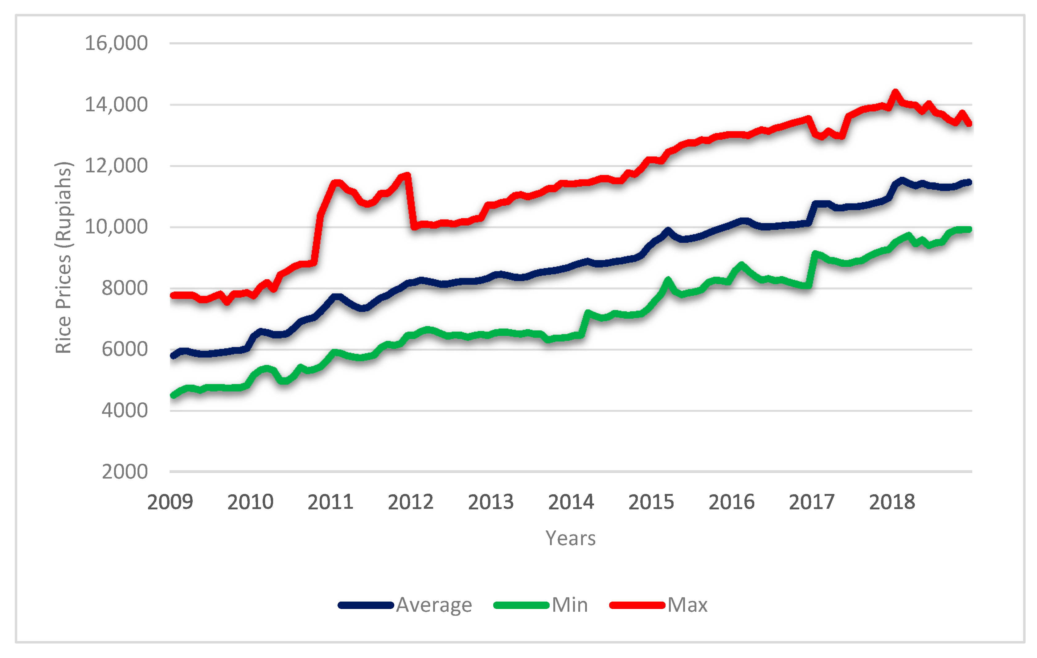
The data used in this study are rice prices (in kg per rupiah) from January 2009 to December 2018 (
Figure 1). The logarithmic return series was calculated from the monthly rice series prices to check price volatility. The development of rice price data is measured nationally in 33 provinces in
Table 1, with variations. It can be seen that the average price of rice is Rp. 8823.12, with a minimum price of Rp. 4404.00 and a maximum price of Rp. 14,422. Ten years of values are presented as the values of all markets at the provincial level aggregated from all 33 locations to become the national price.
The return series shows a negative skewness and a kurtosis coefficient of around 1.288, and 14.501, which means that the return series value is very leptokurtic. The kurtosis value indicates that the return data on rice prices have a heteroscedasticity problem. We can interpret this to mean that the distribution of the economic variables analyzed has a tail that is denser than the normal distribution. The skewness value of rice prices and the return value are greater than 0, which means that the data distribution slopes to the right and tends to accumulate at a low value. The estimated rice price data are the return data, because they are calculated based on current and past prices using natural logarithms.
The observed rice prices showed an increasing trend during the study period and had high volatility from the observed absolute return series under consideration. The average value of all regions is used, but the figure shows the maximum and minimum values to see the difference. This difference indicates a huge boundary between the average and the highest and lowest values, due to regional geographic differences. Based on the community’s economic carrying capacity, it is known that not all regions have rice production.
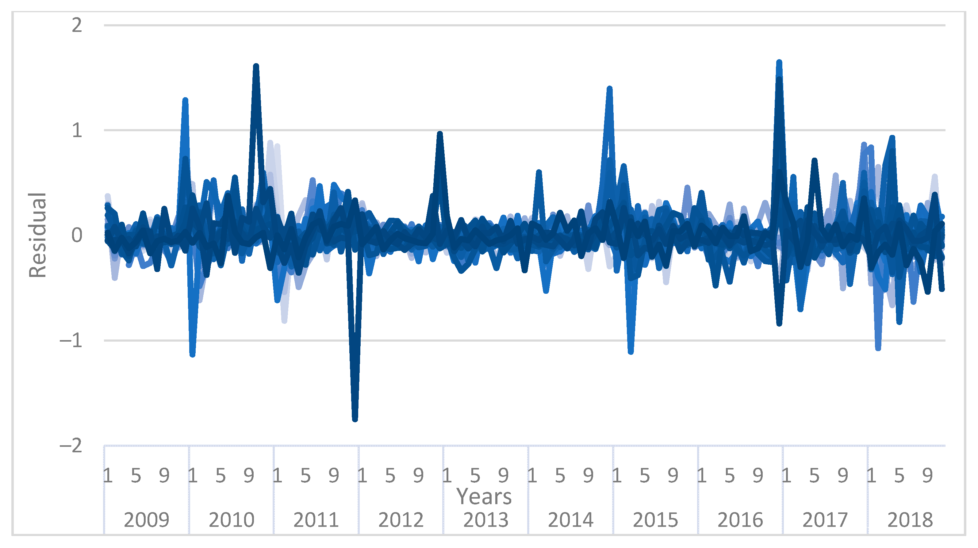
The residue shows the volatility in rice prices in the market through the log return value;
Figure 2 shows years when the volatility rate slopes, but several periods have high fluctuation values. This condition indicates that unstable volatility is a pattern to be concerned about, as well as increasing prices, especially at the farm level.
4.2. Unit Root Test, Box–Jenkins Model, and ARCH Test
The ARCH-GARCH model can be built after going through several stages of estimation. The first is to test the stationarity of the data to be analyzed. Second, we identify the Box–Jenkins model (AR, MA, ARMA, and ARIMA) by observing the stationarity test results. Third, we test the ARCH effect of the selected Box–Jenkins model. The ARCH effect test will determine whether the selected model can be further analyzed using the ARCH-GARCH model. Fourth, we estimate the ARCH-GARCH model by choosing the best model. Finally, we use the normality test to evaluate the model and perform the ARCH-LM test to determine whether the selected ARCH-GARCH model is free from the ARCH effect. If desired, forecasting can be done on the ARCH-GARCH. The data on rice prices for estimation of volatility value were tested for stationarity. The stationarity test can be done by looking at graphs or correlograms, or doing the unit root test. The unit root test can use many test tools, one of which is the augmented Dickey–Fuller (ADF) test. The stationarity test is essential to do on time series data so that the resulting data is predictable and unbiased, and it can be carried out at the level, first difference, and second difference. Research on rice prices in Indonesia shows that the data are stationary in the first difference.
The Box–Jenkins model was determined after the stationarity test was carried out, including auto-regressive (AR), moving average (MA), auto-regressive moving average (ARMA), and auto-regressive integrated moving average (ARIMA) models. If the data are stationary at the level, then the estimation model uses ARMA; if the information is stationary in the first difference, it uses ARIMA. The model was made for all 33 provinces, showing that the variable is stationary at the first difference level, so the Box–Jenkins model used is ARIMA (
Table 2). The best model is chosen after doing several ARIMA model simulations. The criteria for selecting ARIMA are based on significant estimation coefficients, with the largest R-squared and adjusted R-squared, the smallest AIC and SIC values, and relatively small values of standard error of regression and sum square residual.
The ARCH-GARCH model can calculate volatility if there is an ARCH effect on the selected ARIMA model. The ARCH effect test is intended to determine whether there is a heteroscedasticity model to determine the actions to take for the next step.
There is a problem in the three rice price variables of all provinces. It can be seen that the probability value of each food price is less than 5% of the real level, so it can be concluded that there is a heteroscedasticity problem in the rice price variables. The heteroscedasticity problem can be solved using the ARCH-GARCH model. A probabilistic value above 0.05 indicates homoscedasticity. Testing the ARCH effect (
Table 2) shows that there are models with a heteroscedasticity problem for six provinces, because the ARCH effect is found. The ARCH effect found in each of the best ARIMA models indicates that the calculated volatility varies over time.
4.3. Rice Price Volatility
The ARCH effect in the ARIMA model will determine the model for further analysis using ARCH-GARCH.
Table 3 shows six models of rice prices at the provincial level, namely West Sumatra, Babel Islands, Central Java, Central Kalimantan, Central Sulawesi, and Maluku. The volatility values of the six models were processed using the ARCH-GARCH model. The best ARCH-GARCH model was selected based on the criteria. All significant coefficients in the variance equation have the most considerable log-likelihood value and the smallest AIC and SIC values. They have positive values for all coefficients in the variance equation. Based on the existing criteria, the ARCH-GARCH model was selected for rice price variables.
The GARCH model is the best for the three food commodities studied. After selecting the best GARCH model, the next thing to do is to evaluate the model. Model evaluation can be done through the normality test by paying attention to the Jarque–Bera statistical value. The results of the Jarque–Bera statistical test can be seen in
Table 3. The normality test results show that the Jarque–Bera value is statistically significant, which means that the model error is not normally distributed. All ARCH-GARCH models for each variable were tested for normality and show that all of their errors are not normally distributed, so the ARCH-GARCH model is still the best.
The last part is to evaluate the model using the normality test. The value seen is Jarque–Bera. If the test results are significant, the model error is not normally distributed. The model is again tested if it still has an ARCH effect by using the ARCH-LM test. The probability score is greater than the 5% confidence level (α). If there is still an ARCH effect, the model must be revised until it obtains a result that is free from the ARCH effect.
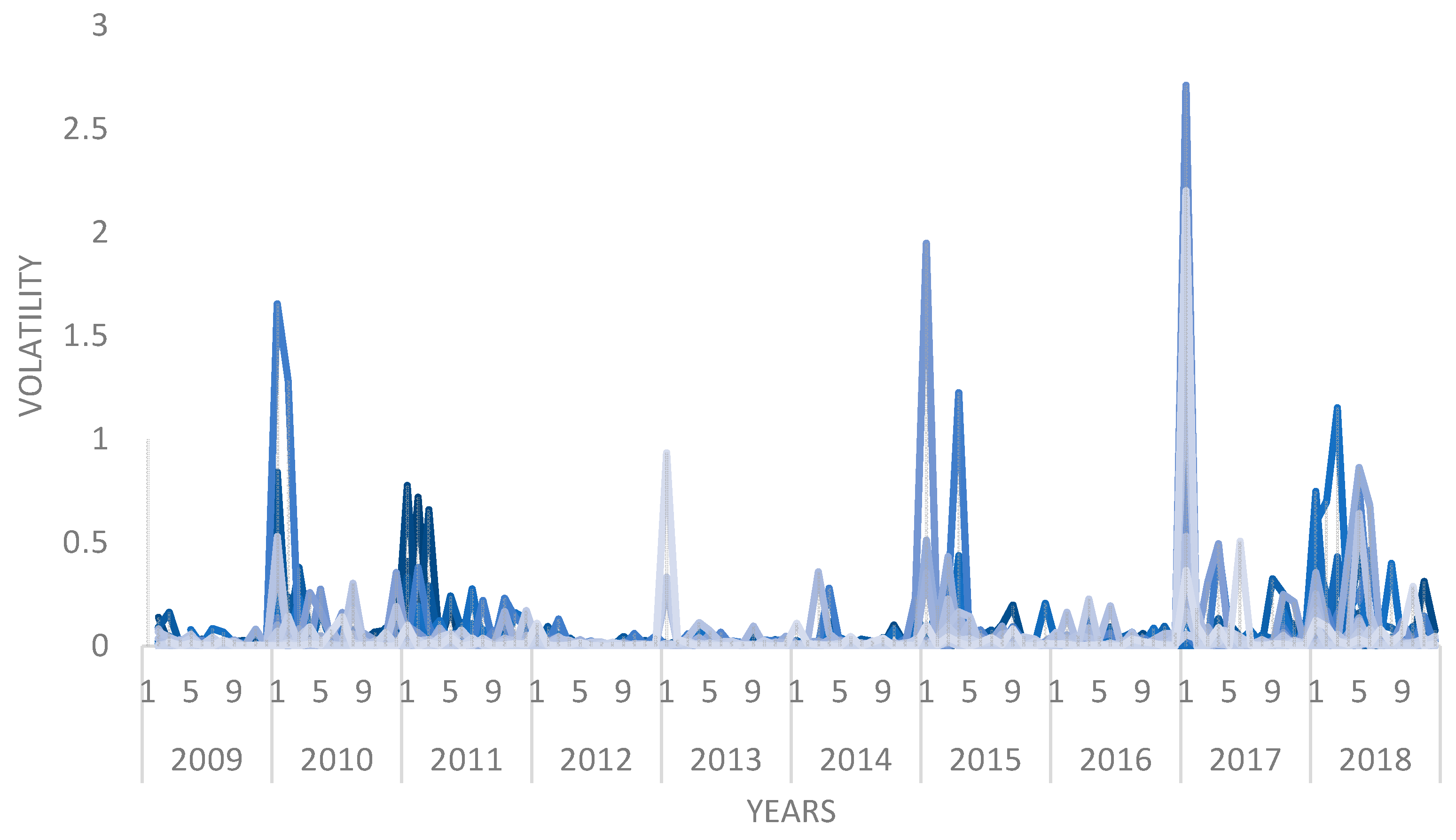
Rice price volatility in this section uses the square of the logarithmic standard deviation of provincial monthly food price. Values below the average of 0.03 are rice prices with little volatility. So, it can be seen that rice has exceptionally high price volatility in several periods (
Figure 3). The period with high volatility over the longest time refers to the value above the standard deviation from August to September 2017. High volatility values also occurred from May to December 2015 and from April to November 2010. Some values also had very high volatility. The conditions occurred in several regions with price volatility, such as in January to February 2016 and January to February 2010.
4.4. Effect of Macroeconomics and Climatic Determination for Rice Volatility
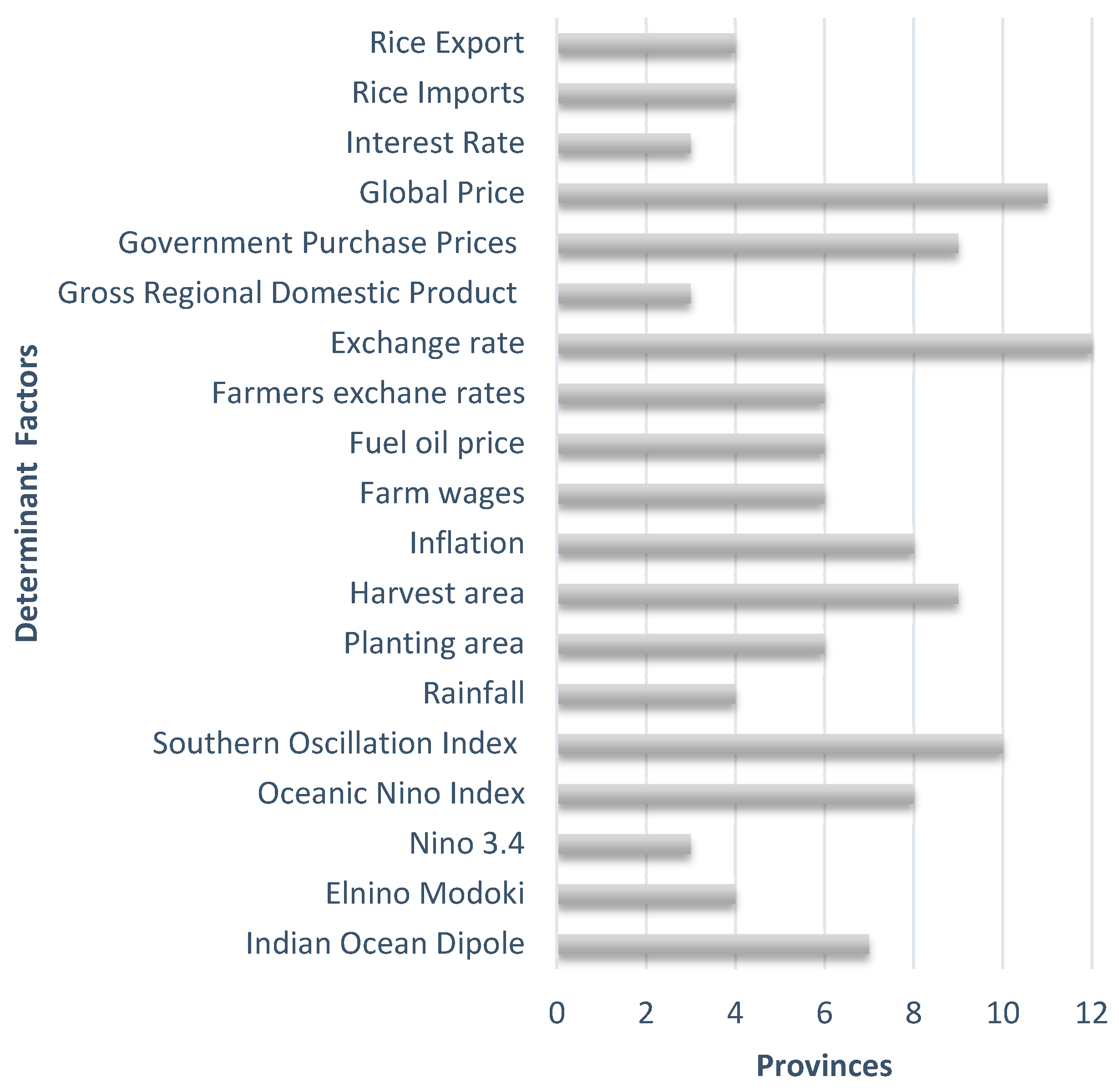
The data show the most dominant influence on the volatility of rice prices in each province (
Figure 4). To make it easier to accumulate, the most dominant influencing variables with various determinative factors are not shown here. We can get an overview of the most dominant climate variables and macroeconomic groups that affect rice prices at the provincial level. The results show that the rupiah exchange rate against the dollar dominates the pattern of rice price volatility at the regional level. However, if it is related to local influences, only four provinces have a significant influence. Global rice prices also remain a determinant in influencing price volatility at the national level. Government intervention on prices is considered as one way to control the level of volatility in line with the 10 provinces as a whole group.
In the climate variable, a component that is directly considered related to agriculture and the availability of rainfall, significantly affects four provinces. Regarding the triggering factors, it is known that the southern oscillation index has the most influence on ten 10 provinces in Indonesia. This is inseparable from the prevailing climate conditions in the central and eastern parts of Indonesia. The second component is the oceanic Nino index, which also shows El Nino and La Nina’s effects on rice price volatility, especially in eight provinces. The trigger for wet and dry conditions for the western region, the Indian Ocean dipole, strongly affects seven areas.
Inflation and gross domestic regional product are two of the macroeconomic indicators. Inflation was chosen as a variable for macroeconomic performance because it is one of the economic problems affecting the real sector. In the entire industry, inflation affects government spending and taxes. In the monetary sector, inflation can affect interest rates and the money supply. The real and financial sectors are the two main sectors in the economy. If inflation occurs, the impact will spread to various economic actors such as the government, households, and companies. The inflation data used in this study represent general price inflation, affecting eight provinces.
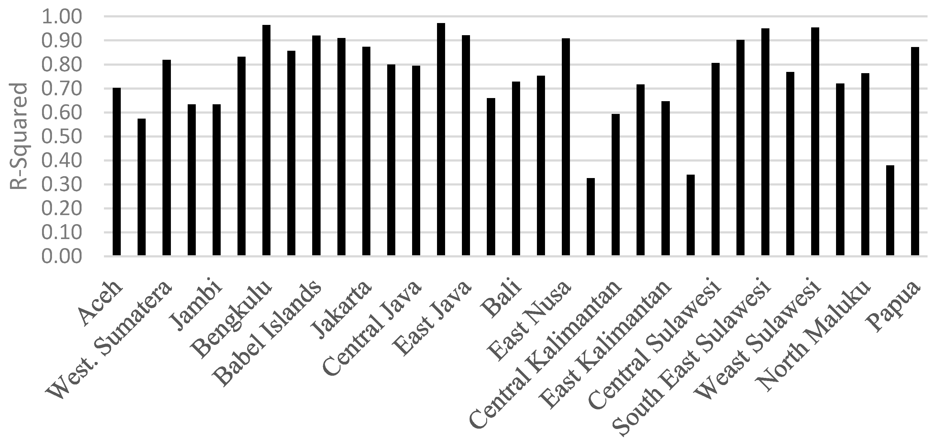
The model can effectively describe rice price volatility in combination with macroeconomic components and climatic conditions, but not all regions are well represented, as seen in
Figure 5. Three provinces respond less well to the R-squared value, namely West Kalimantan, North Sulawesi, and West Papua. This was reflected in the climatic factors, because these three regions have unique patterns and the least measurable agriculture components. Provinces that are based on food agriculture show an average value of 70% in the Java Island region, except Banten Province does not respond well. There are two perceptions through the R-squared model: only a few dominant variables influence an area, or most of the variables affect it. The Riau Islands region was influenced predominantly by the value of wages, and Papua by fuel oil price.
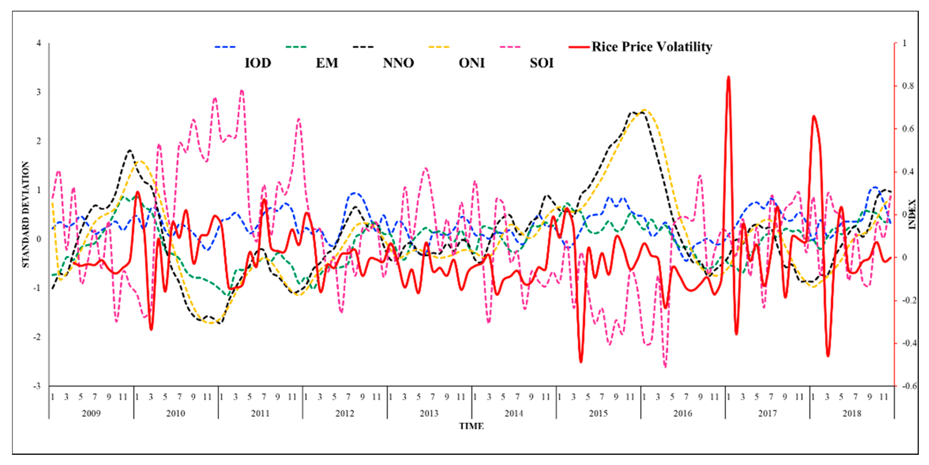
In analyzing Indonesia’s natural factors, the seasonal factor was put into a series to be compared with the level of price volatility (
Figure 6). Years with substantial fluctuations, such as the end of 2009 to early 2010, show the strong influence of SOI and Nino 3. The impact of El Nino and La Nina conditions on agricultural economic conditions in the Indonesian region is emphasized. The variations are quite diverse compared to the robust EL Nino in 2015, when price volatility was quite intense at the beginning of the year. La Nina has shown a more dominant influence, such as in 2006, and the volatility of rice prices tended to persist in 2012 to 2014, which was also marked nationally by fluctuations in climate dynamics that were not too extreme. The volatility shock at the end of the data period in 2018 was only shown to be an effect of La Niña.
5. Discussion
Increasing food prices at the global level is also in line with rice prices in the Indonesian market, which have shown an increasing trend in the last 10 years and a tendency to decline with difficulty. The same threat could be faced in other countries in the world [
1], because it is relatively tricky to control price reduction. The world population continues to increase, as noted in [
3], which tends to be the same condition in Indonesia, and its impact means an increasing need for access to food. The fact that the population continues to increase will undoubtedly lead to an increase in food needs, and coupled with the number of poor people, price shocks can be a threat to environmental sustainability. Extreme volatility of rice prices has been seen in several periods in the Indonesian market. It also causes difficulties in accessing food by the public, as described in [
5]. Although the results obtained show that global market conditions do not influence Indonesia’s rice market, this is different from research that tends to show better food security [
10].
It is feared that global climate change will increase the threat to food availability [
22]. The carelessly designed climate mitigation policies can increase the number of people at risk of hunger [
2]; a volatility model that performs better with climate and macroeconomic variables is expected to reduce this gap with more relevant information. In line with [
38], the result supports the global goal of food production efforts to be carried out simultaneously with climate change mitigation. The effects of the five climate indices used in this paper show that climate has a strong influence on rice market conditions. These conditions are directly caused by decreased production and many other things that need to be studied in depth in the future. It is successfully confirmed that rice price volatility shows a similar pattern or a time difference, but with a strong correlation. Threats arising from changes in the global environment are in line with findings showing that the readiness of the market system, especially for people with low income, is not the object with the most loss [
27]. A government that can control price volatility needs to prepare the best scenario to reduce social impacts.
A model used to measure the volatility of rice prices can optimally present outputs at the provincial level. The unit root test [
52] with ADF is still a practical test to measure the magnitude of the stationary variables. The choice of a time series model with ARIMA is known to be dominant in the research area. As obtained from previous research [
51], rice at the provincial level in Indonesia has also been measured well. Measuring the ARCH effect with ARCH-LM can measure the heteroscedasticity effect in order to determine the six provinces for which the GARCH model must be used. The best model besides GARCH is EGARCH, which can respond to lagged errors in asymmetry so that the residue for rice price volatility can be measured as a whole. Further integration of the different models is needed to better explain multi-level and cross-scale feedback in food systems [
64]. Cumulatively, the picture of national rice price volatility can be seen by combining all data at the provincial level.
The climate data approach used to identify the value of price volatility shows relatively strong interactions. These price shocks appear in line with the time series of climate anomalies. A strong El Nino effect, as measured by the ONI and Nino 3.4, indicates strong price shocks in the Indonesian region from late 2009 to the early La Nina conditions that followed. Volatility returned to a slope but then La Nina strengthened in late 2010 to early 2011, causing the volatility to bounce back. These two things show the strength of the interaction between Indonesia and climate dynamics in the Pacific Ocean, in the form of both rainfall and an increase in extreme events that impact price volatility. The strong La Nina year in 2015 also showed intense price volatility. However, apart from climatic factors, such as rice prices, volatility in 2018 tended to be dominated by macroeconomic factors. El Nino and La Nina affected rice conditions but did not cause fluctuations, because conditions neutralized the value of price volatility [
33,
34]. The development of climate dynamics can be identified, which can influence volatility.
The GARCH method can provide an overview of volatility in the level of shocks to the food economy at a regional scale, accompanied by various determinants in each region that can be used for policymaking. On rice price volatility, the average R-squared of provinces in Indonesia is 0.75, an excellent value in describing variables that explain the significance of volatility. In general, it was 25% defined by other components nationally. High volatility is proven to be always due to the influence of macroeconomic and climatic features. This situation increases the risk for lower class farming communities. The low exchange rate of farmers indicates that the emergence of rice price volatility will have a significant impact on their household economies.
This research is in line with [
39,
65], marked by global prices in local economic conditions. Still, it is found that the effect of exchange rates is more dominant than the level of international prices and the number of imports. It is in line with [
40], which showed that increasing prices on a local scale due to the global food crisis and long-term effects are still being felt. This situation can always be helped by increased farmer value and controlled inflation, but what needs more attention is the very high price volatility that accompanied the global crisis in 2008. Factors such as climate dynamics can also worsen local conditions. Policies to deal with similar situations are needed to address the impact on the poor. Similar to [
66], government intervention in the purchase and distribution of food can empirically control price volatility. From the results of the study, ten provinces were dominantly controlled by government intervention. The increase in the price of imported rice has impacted poor households more than wealthy households [
41], one of the efforts to increase food security by reducing global shocks’ impact on food price imports.
The rupiah tended to be stable from October 2009 to May 2013, and depreciation occurred again in 2013, with a sharp decline in value at the end of December, when there was a deficit balance of payments and foreign investors’ flight uncertainty over the debt crisis in Europe, foreign exchange liquidity, and a reduction in stimulus in the United States. Rupiah depreciation was recorded twice. The first was in 2015 due to the global impact of the protracted crisis in Greece, which affected global markets, the recovery of economic conditions in the US, and domestic needs undergoing government transition. Various aspects influenced the depreciation of the rupiah. A government policy package was carried out, plus there was an increase in prices followed a policy to abolish fuel subsidies in 2015. At the end of the year, there was a decline in global oil prices to help the rupiah remain stable. However, several areas were hit by high volatility at the provincial level, coupled with decreased rice availability due to El Nino. The dynamics of exchange rates was in line with [
19] and price uncertainty were also found following an investigation by [
40].
In 2018, with the trade war between the US and China and the current account deficit, the rupiah weakened again. Bank Indonesia implemented a monetary policy by raising the benchmark interest rate to 5.5%. In October 2018, the rupiah reached its highest value in the 2009–2018 period, resulting in volatility shocks that were almost evenly distributed in all provinces. The inflation rate has been shown to have a strong influence on price volatility, including rice supply availability. The agricultural area does not always indicate a dominant effect, although this is very significant in some areas. However, on a large scale, in Indonesia’s case, the export and import factors of rice do not have a strong influence on the level of price volatility, including GRDP, which only affects provinces that fully legalize agriculture with low farmer income levels. This study is slightly different from [
43], which could not reflect macroeconomic indicators, but this may also be caused by differences in measurement methods. The purchasing power of farmers may not increase as long as price volatility can be kept at a safe level, in contrast to [
46], which recommended expanding the wage level. However, in the context of household food security, how to maintain the availability of rice supply and the ability to access it can be measured by price volatility. The government purchase price policy can be maintained because it has a reasonably dominant influence in several provinces, but it needs to be accompanied by better policies.
Agricultural production has been shown to influence the volatility of rice prices. When the volatility of rice prices experiences shocks, the poor are the most affected, many of whom reside in the study area. If food shortages increase, there is the potential for agricultural expansion that will threaten increased deforestation for both agricultural and other purposes. Increasing the food stock by enlarging the agricultural area is not recommended, advisable to exploit the harvest and enforce policies [
67]. Farming areas that tend to be homogeneous also do not positively affect food price stability, impacting food access. Biodiversity can coexist with rice farming systems in the Indonesian region. However, it is still necessary to have good management and increase agricultural variation to maintain soil fertility. Rice farming threatens biodiversity and environmental sustainability. When viewed from the high level of rice price volatility in times of climate threats and macroeconomic conditions, this research is very encouraging in terms of increasing the choice of food availability, which is positive for biodiversity. Low agricultural income affecting price volatility will also be related to the available labor force. Options will arise when agriculture is no longer attractive to the younger generation, the industrial world will increase, and migration will continue to increase the deforestation rate. On a broader scale, if rice price stability can be maintained, then policy efforts that emphasize increasing rice production can be changed, because the consequences that arise from changes in agricultural systems are increased with the use of fossil fuels and monoculture agriculture, and increased greenhouse gases. Even though this situation is global, environmental sustainability must be maintained.
6. Conclusions
For the first time, rice price volatility was measured by involving climate dynamics and macroeconomic variables. For most Asian countries, the results are significant because food security is often linked to staple food availability for the community. Especially after the global food crisis that caused global food prices to jump, knowledge about maintaining price volatility is fundamental, mainly to not interfere with the ability of the poor to provide food for their households. With the threat of future climate change, knowledge of rice price controlling factors must be improved. Attention must also be paid to reducing poverty, which is closely related to the lack of sustainability, due to the higher potential for environmental damage, due to land clearing to meet food needs.
The model for measuring rice price volatility has high complexity, and it depends on many variables. An interrelated pattern can be obtained using a combination of market price data at the consumer level and macroeconomic variables with climate variables. The use of models for each province also shows better results than using only one ideal setting for the entire nation. Estimates and predictions of rice price volatility can be used to support the process of determining policies that promote the level of access to food for the community.
The ARCH-GARCH model was successfully built after going through several stages. The stationarity ADF test shows a stationary value in the first difference. The Box–Jenkins model for rice prices in Indonesia uses the ARIMA model. ARCH-LM is also proven to be useful in testing the ARCH effect, so that some models continue to use the GARCH method, and some also efficiently use EGARCH. The model can also be used to describe the dependent variable that affects the level of price volatility. The price of rice at the market level in Indonesia demonstrates an increase in value. The volatility that has arisen in the last few years is also getting steeper. In general, low-income farming communities will have a substantial impact on the economy at the household level. It is feared that employment in agriculture will be abandoned because the average farmer’s income is low.
The macroeconomy is still the most significant factor in Indonesia influencing the levels of price volatility, exchange rate, global price, GPP, and harvest areas as the most dominant factors. These results indicate that although import factors do not predominantly influence the Indonesian market, shocks in the exchange rate can affect rice price volatility. Other factors that are also quite dominant include the inflation rate, farmers’ exchange rate, fuel oil prices, and farm wages. Even though they are not as prevalent as the main factors, they can be considered mainly for their impact on the local market level because they can also appear on the micro level.
The influence of climate on rice prices is also shown through the indices used, with the SOI and ONI values being the most dominant. This shows that the influence of El Niño and La Niña is the primary driver of the volatility of rice prices in Indonesia, so in the future, we must look not only at the impact of climate on rice production, but also at macroeconomic factors. The influence of phenomena in the Pacific and the effect of IOD, which is a phenomenon in the Indian Ocean, are also quite dominant in influencing rice price volatility in several regions. The combination of climate index data and macroeconomic variables successfully represents the characteristics and patterns of volatility at the provincial level in Indonesia. Of the 33 provinces analyzed, only 3 provinces had a group of representation below 50%. An explanation of other variables that may arise due to the region’s uniqueness is needed. However, for provinces that are well described, they can start to use the climate and macroeconomic approach to maintain the sustainability of both agriculture and the economy of the community.


 ,
, 


