Abstract
In this paper, we apply a combined revenue sharing and buyback contract to investigate the channel coordination of a two-echelon supply chain with a loss-averse retailer. Since loss-averse decision makers usually take on more risks, the Conditional Value-at-Risk (CVaR) measure is introduced to hedge against it and the retailer’s objective is to maximize the CVaR of utility. We obtain the retailer’s optimal order quantity under the combined contract. It is shown that there is a unique wholesale price coordinating the supply chain if the retailer’s confidence level is less than a threshold that is independent of contract parameters. Moreover, a complete sensitivity analysis of parameters is carried out. In particular, the retailer’s optimal order quantity and coordinating wholesale price decreases as the loss aversion or confidence level increases, while it increase as the buyback price or sharing coefficient increases. Furthermore, there exists the situation where the combined contract can coordinate the chain even though neither the revenue sharing nor buyback contract can when the contract parameters are constrained.
1. Introduction
Sustainable supply chain management has drawn a great deal of attention in recent years and has been studied in various contexts (e.g., [1,2,3,4,5,6,7,8]). Sisco et al. [9] define it as jointly considering multiple effects (e.g., environmental, economic, and social) and implementing friendly manufacturing practices during the product life cycle. Choi and Chiu [10] classify supply chain sustainability into economic and environmental sustainability, where the former refers to a supply chain’s sustainable operation ability. However, as is well known, double marginalization prevailing in supply chain management creates supply chain inefficiency. To solve this problem, various contracts such as buyback, quantity flexibility, and revenue sharing that can coordinate the supply chain have been proposed to provide incentives to adjust the members’ relationship. Cachon [11] and Hezarkhani and Kubiak [12] provide good surveys on this topic. Cachon [11] identifies that there are several key conclusions in the supply chain contracting research: Coordination failure is common and its consequence is context specific; multiple kinds of contracts are capable of coordinating the chain and arbitrarily dividing profit; and managing incentive conflicts can lead to Pareto improvements. Hezarkhani and Kubiak [12] find out that the decision makers are assumed to be rational, risk-neutral, and profit-oriented in most of the literature. That is, their objectives are to maximize their own expected profits or minimize their own expected costs. Nevertheless, there are many counter examples implying that the decision makers do not always practice as the risk-neutral models predict (e.g., [13,14,15,16,17]). For example, through experiments, Schweitzer and Cachon [14] and Zhang and Siemsen [17] show that subjects often underorder a high-profit product and overorder a low-profit product, which is called pull-to-center effect. Thus, developing alternative choice models instead of risk neutrality to represent more realistic situations is becoming increasingly important. Within this research stream, many studies have deviated from this assumption and incorporated loss-averse preferences into supply chain models (e.g., [18,19,20,21,22]). Loss aversion is the key feature of Prospect Theory proposed by Kahneman and Tversky [23], and means that people are more averse to losses than the same amount of gains. Since loss aversion is intuitively appearing and is supported in many fields, supply chain management with loss aversion has gradually attracted increasing attention and plays an important role in a manager’s procurement strategy.
Although models based on loss aversion provide useful guidance to managers on their optimal inventory decisions, they are generally studied within the expected utility theory framework and the decisions can be made to maximize the expected utility. However, some studies on portfolio management indicate that loss-averse investors usually take on more risks (e.g., [24,25]). In view of this, a few recent works on the inventory problems consider the risk management of the loss-averse decision makers and then incorporate other objectives rather than utility maximization (e.g., [26,27,28]). For instance, Xu et al. [27] introduce Conditional Value-at-Risk (CVaR) measure into the loss-averse newsvendor problem. They formulate the CVaR of utility and demonstrate that the loss-averse newsvendor’s ordering policy with this CVaR objective is significantly different from that with an expected utility-maximizing objective. They also point out that the CVaR of utility exhibits some desirable properties as a risk measure. Motivated by their work, some interesting questions naturally arise: (1) How does the loss-averse retailer determine the optimal order quantity under a CVaR criterion in a supply chain? (2) What impacts will the retailer’s loss-averse preferences and risk attitude have on the supply chain’s operational decisions? (3) How does one coordinate the supply chain when this CVaR criterion incorporated?
To address the above issues, we try to apply a combined revenue sharing and buyback contract to investigate the channel coordination of a two-echelon supply chain. The manufacturer is a supply chain leader and can diversify their assets across multiple firms, then is assumed to be risk-neutral. The retailer is a follower and the income depends highly on their principal, and then is assumed to be loss-averse. Although this setting of one risk-neutral supplier and one retailer with preferences is adopted in many supply chain contract models, the retailer is generally assumed to be loss-averse and the objective is to maximize the expected utility (e.g., [18,19,20]), or risk-averse and the objective is to maximize the CVaR of profit (e.g., [29,30,31]). Different from them, we simultaneously consider the loss aversion and risk management, and the CVaR measure is introduced to hedge against the loss-averse retailer’s risk. The retailer’s objective is to maximize the CVaR of utility under the combined contract. To the best of our knowledge, this model has not been considered in the literature. In particular, Zhao et al. [29] have adopted this combined contract to study the supply chain in risk-averse setting and clearly demonstrated that this combined contract has advantages over both buyback and revenue sharing contracts in terms of supply chain coordination and profit allocation. Although their research is most related to ours, they only take into account the risk management and fail to consider the retailer’s loss-averse preferences. Moreover, Yang et al. [30] also investigate the supply chain coordination with CVaR criterion, but they only take into account several single contracts and fail to consider composite form as well as loss-averse preferences. Therefore, our model can be thought of as an extension to the above two works. The loss-averse retailer’s optimal ordering policy under the combined contract is firstly obtained. Besides, the impacts of the retailer’s loss aversion and confidence levels on their expected utility under the optimal order quantity are investigated. Then whether the contract parameters can be set to coordinate the supply chain is analyzed, and the sufficient condition of coordination is established. Finally, we compare the performance of this combined contract with both its component contracts, and show that the former has an advantage over the latter when contract parameters are restricted. Our results indicate that when adopting a combined revenue sharing and buyback contract, the supply chain with a loss-averse retailer under a CVaR criterion can be coordinated by setting a proper wholesale price. Thus, double marginalization is eliminated, and the supply chain achieves its optimal performance and becomes sustainable.
The rest of this paper is organized as follows. In Section 2, we review the literature related to the present paper. In Section 3, we describe our model. Section 4 discusses the retailer’s optimal policy under the combined contract and Section 5 investigates the issue of supply chain coordination. In Section 6, numerical experiments are conducted to validate our analysis. In Section 7, we come to the conclusion and future research directions.
2. Literature Review
There are three research areas that are most relevant to our study, namely the supply chain contract models incorporating loss aversion, supply chain contract models incorporating risk aversion, and the inventory models incorporating both loss aversion and risk management.
The literature on the supply chain contract models with loss-averse agents is first discussed. Wang and Webster [18] consider a combined contract in the supply chain with a loss-averse retailer and show there exists a special class of coordinating contracts that are independent of demand. Chen et al. [32] investigate a supply chain via an option contract and derive the retailer’s and supplier’s optimal policies. They also show there always exists a Pareto contract. Zhai and Yu [19] use a robust approach to study supply chain coordination when the distributional information of demand is limited. Xu et al. [20] investigate the retailer’s optimal option purchase decision under emergent replenishment. Chen and Xiao [33] design a buyback-setup-cost-sharing contract to study the supply chain coordination under three different ordering policies. Zhang et al. [34] investigate the loss-averse supplier’s preferences and contract performance between buyback and revenue sharing contracts. Moreover, since supply chain risk managementhas received increasing attention over the past few decades (e.g., [35,36]), some researchers have incorporated supply uncertainty into the supply chain contract models. For example, Xie et al. [37] propose a revenue-cost-sharing contract to study the supply chain with a loss-averse retailer, yield uncertainty, and marketing effort. Du et al. [38] also consider a supply chain with yield risk, where both the supplier and retailer are loss-averse. Both parties’ optimal decision making under the wholesale price contract and the impacts of loss aversion on them are investigated.
Second, the present paper is also related to the literature on the supply chain contract models with risk-averse agents. Although there are multiple research methods for risk management including Mean-Variance (e.g., [39,40]), VaR (e.g., [41,42]), and CVaR, CVaR has drawn a great deal of attention and been widely adopted in the literature because of its better computational characteristics [43]. We briefly review the models under CVaR criterion that are most relevant to ours. Yang et al. [30] consider four different contracts and show that a supply chain with a risk-averse retailer can all be coordinated. Zhao et al. [29] extend their work by using a combined revenue sharing and buyback contract. They also demonstrate this combined form has advantages over both component contracts. Chen et al. [44] consider random default probability and analyze the effect of trade credit on supply chain coordination. In the case with and without horizontal price competition, Hsieh and Lu [31] investigate the manufacturer’s return policy in a supply chain with two risk-averse retailers and price-dependent demand. Xie et al. [45] assume the retailer takes mean-CVaR as their performance measure and demonstrate that three common types of contracts can coordinate the chain under mild conditions. Wu et al. [46] consider a commitment-option contract and analyze the impact of risk aversion on the manufacturer’s optimal decisions. Wang et al. [47] study a supply chain under option contract where two risk-averse retailers compete for demand.
Finally, the present paper is related to the literature on inventory models incorporating both loss aversion and risk management. Although the inventory research with loss-averse or risk-averse preferences has made a lot of achievements (e.g., [48,49,50,51]), the publications jointly considering both factors are relatively limited. Xu et al. [27] study the loss-averse newsvendor problem under CVaR criterion and present management insights on how to balance loss aversion and fill rate. Xu et al. [52] investigate the newsvendor problem with backlogging and the objectives are to maximize the expected utility and CVaR of utility, respectively. The optimal ordering policies are obtained and the impacts of backlogging on them are analyzed. Sun and Xu [53] propose a new loss aversion utility function composed of losses weighted by a coefficient and profit in the newsvendor model. The optimal order quantity maximizing the CVaR of utility is decreasing in loss aversion and confidence levels. Chan and Xu [28] extend their model by considering shortage cost and find that the order quantity may increase when loss aversion or confidence level increases. Liu et al. [54] also adopt this utility function to study the newsvendor problem with backlogging. Moreover, Xu et al. [26] propose a legacy loss defined either as the loss for excess order or the shortage penalty, and study the newsvendor problem under different objectives.
3. Model Description
The paper considers a supply chain composed of a large manufacturer and a small retailer. The risk-neutral manufacturer is the leader and announces a supply contract before the selling season. The loss-averse retailer facing random customer demand is the follower and makes the ordering decisions if they accept it. Then the manufacturer begins to produce and provides the quantity ordered. The retailer sells the products directly to the customers and unsold units will be salvaged at the end of the period. Notations concerned in this paper are listed in Table 1.

Table 1.
Summary of notations. CVaR: Conditional Value-at-Risk.
To provide a benchmark, we first take into account an integrated supply chain where the risk-neutral manufacturer owns a retail channel and acts as a central controller. In this case, the manufacturer faces a newsvendor problem and it is well known that the optimal production quantity is (e.g., [18]):
In a decentralized chain, the manufacturer and retailer are independent and seek individual performance maximization. For any given supply contract, the loss-averse retailer is assumed to take the CVaR of utility as the performance measure. When the retailer’s profit is , their utility is:
where reflects the degree of the loss aversion, and the retailer is loss-neutral when . This function has been widely adopted in supply chain management due to its simplicity (e.g., [18,37,48,49]).
It follows from Xu et al. [27] that the VaR and CVaR of utility are defined as:
and
where is the retailer’s confidence level and reflects the degree of the risk aversion. Note that when , the CVaR of utility reduces to the expected utility, which is the objective function in many inventory models based on loss aversion (e.g., [18,20]). When , the CVaR of utility reduces to the CVaR of profit, which is the objective function in many inventory models based on risk aversion (e.g., [29,47]). Furthermore, when both and , the CVaR of utility reduces to the expected profit, which is the objective function in many inventory models based on risk neutrality. Then the loss-averse retailer’s ordering problem when incorporating risk management can be expressed as:
From Xu et al. [27] we can obtain that the optimal order quantity of the retailer facing a newsvendor problem is less than the system-wide optimal production quantity due to double marginalization, loss aversion, and risk aversion. Thus, the supply chain behaves poorly and is inefficient. Our purpose is to design a proper contract that can eliminate these negative effects and coordinate the chain. That is, the contract can induce the retailer to order the system-wide optimal quantity (e.g., [29,30]).
4. Retailer’s Optimal Policy under the Combined Contract
To coordinate the supply chain, we propose a combined buyback and revenue sharing contract with parameters , and its operation sequence is as follows. The manufacturer charges the retailer w per unit purchased, but the unsold products will be returned to them with price b per unit at the end of the period. Then the retailer shares the fraction of the total revenue over the selling season to the manufacturer and retains the remainder. For simplicity, assume all the retailer’s revenue is shared (e.g., [30]), i.e., the revenue comes from buyback is also shared. Therefore, the retailer actually receives from the customer for each unit sold and from the manufacturer for each unit unsold. It is reasonable to assume , since the retailer will order as much as possible when , and not order when . Note that the combined contract is the buyback one if , and is the revenue sharing one if . Thus both are special cases of the combined contract.
Under this combined contract, the retailer’s profit is:
There exists a break-even quantity of the realized demand, below which the retailer’s profit is negative, that is, incurring a loss. Otherwise, the profit is positive, that is, making a gain. The following theorem gives the loss-averse retailer’s optimal order quantity under the CVaR of utility for a given contract .
Theorem 1.
The CVaR objective of utility for the loss-averse retailer is concave. Thus, there exists a unique optimal order quantity that satisfies:
Proof.
See Appendix A. □
The impacts of loss aversion, confidence level, and contract parameters on the optimal order quantity are as follows.
Corollary 1.
The retailer’s optimal order quantity is decreasing in λ, α, and w, whereas increasing in b and β.
Proof.
See Appendix A. □
This corollary shows that the lower loss aversion or confidence level motivates the retailer to order more products and drives the inventory up. The less loss-averse or risk-averse the retailer is, the larger the order quantity. In particular, the loss-averse retailer’s optimal order quantity is less than the risk-neutral one’s ( and ). Moreover, the retailer will order fewer products when the manufacturer charges a larger wholesale price, and order more when the buyback price or sharing coefficient increases, which is consistent with our common sense. Note that these impacts of individual contract parameters on the order quantity are in accordance with that in the existing research on buyback and revenue sharing contracts. This means that comparing with single buyback or revenue sharing contract, their combined form and the retailer’s preferences do not alter the effects of contract parameters.
Since reduces to the optimal order quantity maximizing expected utility when , then and it follows from (7) that satisfies:
The following theorem characterizes how the retailer’s expected utility under the optimal order quantity changes when loss aversion or confidence level increases.
Theorem 2.
When the order quantity is , the retailer’s expected utility is decreasing in α and λ.
Proof.
See Appendix A. □
5. Supply Chain Coordination
We next study supply chain coordination under a combined contract. That is, whether the manufacturer can set the proper contract parameters to induce the retailer to order . The following theorem shows this is possible under the certain condition.
Theorem 3.
If , then there exists a unique wholesale price that can coordinate the supply chain, where satisfies:
Otherwise, the wholesale price coordinating the chain does not exist.
Proof.
See Appendix A. □
This theorem indicates that the combined contract may coordinate the supply chain with a loss-averse retailer who operates under CVaR. There exists a unique coordinating wholesale price if the confidence level is less than a threshold. That is, if the retailer is not too risk-averse (level is less than ), then the combined contract can induce the retailer to order the system-wide optimal production quantity so that the supply chain can be coordinated. Moreover, it is shown that the coordinating wholesale price relates to the retailer’s loss aversion level, which means that the combined contract designed by Zhao et al. [29] does not coordinate the supply chain any more when considering the retailer’s loss-averse preferences. Note that in the special case when , the proposed contract by this theorem is just the one given by Zhao et al. [29] for risk-averse setting.
We next carry out the sensitivity analysis and investigate the impacts of parameters on the coordinating wholesale price.
Corollary 2.
If , then is decreasing in λ and α, whereas increasing in b and β.
Proof.
See Appendix A. □
When the retailer becomes more loss-averse or risk-averse, the manufacturer must charge a lower wholesale price which can induce the retailer to order more products. However, when the buyback price or sharing coefficient increases, the inventory risk transfers from the retailer to the manufacturer. Thus, the latter must enhance the wholesale price to hedge against the risk.
We have mentioned above that the buyback and revenue sharing contracts are special cases of the combined contract. In particular, the combined contract reduces to the revenue sharing one if , and the coordinating wholesale price is . The combined contract reduces to the buyback one if , and the coordinating wholesale price is . Therefore, when the buyback or revenue sharing contract can coordinate the supply chain, the combined contract can as well. An interesting question is whether there is the case that the coordinating combined contract exists even though neither the coordinating buyback nor revenue sharing one exists. The following theorem shows this may occur when the contract parameters are restricted.
Theorem 4.
Suppose and . If and , then neither the coordinating buyback nor revenue sharing contract exists, while the coordinating combined one exists.
Proof.
See Appendix A. □
6. Numerical Experiments
In this section, we proceed with several numerical experiments to illustrate how the optimal order quantity, coordinating wholesale price, and expected profit change when the loss aversion or confidence level increases. Let , , , and . The demand X follows a truncated normal distribution with a mean of 200 and a standard deviation of 100. To illustrate the impacts of loss aversion and buyback price, we fix , , and vary from 1 to 3. Three different buyback prices are considered: , , and . To illustrate the impacts of confidence level and sharing coefficient, we fix , , and vary from 0 to (from Theorem 3 that the supply chain can not be coordinated when ). Three different sharing coefficients are considered: , , and .
Figure 1, Figure 2, Figure 3 and Figure 4 shows how the parameters affect the optimal order quantity and coordinating wholesale price. Figure 1 and Figure 2 illustrate that for any given buyback price, the optimal order quantity and coordinating wholesale price are decreasing in the loss aversion level. Moreover, for any given loss aversion level, both are increasing in the buyback price. Figure 3 and Figure 4 illustrate that for any given sharing coefficient, the optimal order quantity and coordinating wholesale price decrease in confidence level. Moreover, for any given confidence level, both increase in the sharing coefficient. As a whole, the more loss-averse or risk-averse the retailer is, the less the optimal order quantity and wholesale price are. The higher the buyback price or sharing coefficient is, the larger the optimal order quantity and wholesale price are. These results are consistent with Corollaries 1 and 2. The retailer will decrease the order quantity when the retailer becomes more loss-averse or risk-averse. To stimulate a larger order from the retailer, the manufacturer must charge a lower wholesale price. On the other hand, when the buyback price or sharing coefficient increases, the supply risk transfers from the retailer to the manufacturer. Then the retailer will order more products, whereas the manufacturer will enhance the wholesale price to reduce risk. Moreover, it is also apparent that when the loss aversion or confidence level increases, the degrees of change to order quantity and coordinating wholesale price are affected by the buyback price and sharing coefficient. For example, the curves when are steeper than in Figure 1 and Figure 2, while the curves when are steeper than in Figure 3 and Figure 4. Therefore, a larger buyback price (sharing coefficient) has a weaker (stronger) effect on reducing the order quantity and coordinating wholesale price.
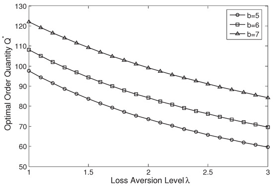
Figure 1.
Impacts of the loss aversion level on the optimal order quantity for different buyback prices.
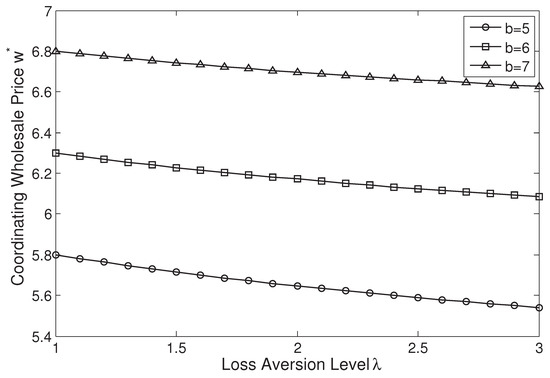
Figure 2.
Impacts of the loss aversion level on the coordinating wholesale price for different buyback prices.
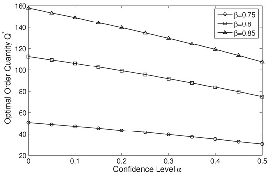
Figure 3.
Impacts of the confidence level on the optimal order quantity for different sharing coefficients.
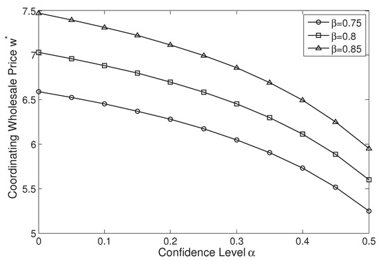
Figure 4.
Impacts of the confidence level on the coordinating wholesale price for different sharing coefficients.
Although the influences of the contract parameters, loss aversion, and confidence levels on the manufacturer’s and retailer’s expected profits are complex in an analytic technique, Figure 5 and Figure 6 illustrate them and present managerial insights. It is shown that the higher loss aversion or confidence level drives the retailer’s profit up while the manufacturer’s profit down, which can be explained as follows. When the retailer becomes more loss-averse or risk-averse, the order quantity is less. To stimulate the retailer to order the system-wide optimal quantity, the manufacturer must share more profit with the retailer. Moveover, when the sharing coefficient increases, Figure 6 shows the retailer gains more profit while the manufacturer gains less, which is consistent with our common sense. However, when the buyback price increases, the phenomenon shown in Figure 5 that the manufacturer gains more profit is counter-intuitive, because one may suppose that they should prefer a lower buyback price to reduce the payment for the unsold products. Although this supposition usually holds for a constant wholesale price, it is not always the case when this price is affected by the buyback price. Since a higher buyback price will make the manufacturer charge a higher coordinating wholesale price (see Figure 2), then they can gain more.
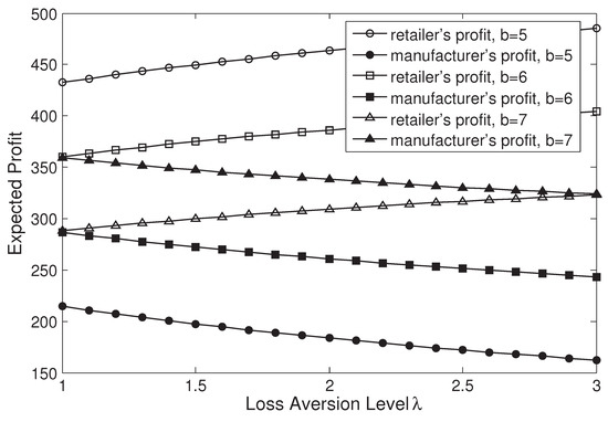
Figure 5.
Impacts of the loss aversion level on the expected profit for different buyback prices.
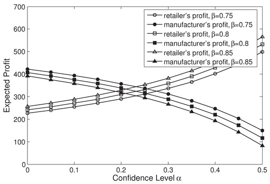
Figure 6.
Impacts of the confidence level on the expected profit for different sharing coefficients.
7. Conclusions
In this paper, we investigated supply chain coordination with a loss-averse retailer. Different from prior research where the loss-averse retailer’s objective is to maximize the expected utility, the retailer was assumed to take the CVaR of utility as their performance measure. A combined buyback and revenue sharing contract was proposed to study this problem. We first characterized the retailer’s optimal ordering policy and analyzed the impact of parameters on it. It is shown that the retailer’s optimal order quantity and expected utility decreased as the loss aversion or confidence level increased. Then the sufficient condition of supply chain coordination was established. If the retailer was not too risk-averse, that is, their confidence level was less than a threshold, then the manufacturer could set a wholesale price to coordinate the supply chain. We also conducted sensitivity analysis of the coordinating wholesale price with respect to contract parameters, loss aversion, and confidence levels.
Our results offer several important managerial implications. First, we found that when the retailer’s loss aversion or confidence level increased, they will reduced the order quantity to hedge against the potential losses or risk, and thus the corresponding expected utility was lower. On the contrary, if the retailer had a lower loss aversion or confidence level, they would order more products and then obtain a higher utility. This result confirms that low return implies low risk and vice versa, thus the retailer should strike a balance between them. Second, when the contract parameters are constrained, there is the situation where the coordinating combined contract exists even though neither the coordinating buyback nor revenue sharing one exists. Thus the combined contract has an advantage over both component contracts in terms of supply chain coordination, and has more opportunities to coordinate the chain. In addition, this combined contract is composed of two well-known contracts and is easy to implement in practice. Third, note that Yang et al. [30] and Zhao et al. [29] have examined the supply chain coordination under single and this combined contracts in risk-averse setting, respectively. The models in the above two works are special cases of ours. In contrast to them, our results indicate that the contract designed by them does not coordinate the supply chain any more when considering loss aversion. Therefore, loss-averse preference is a very crucial factor to set the coordinating contract parameters and has an important effect on supply chain coordination.
There are several possible extensions of this research. First, the reference point in the loss aversion utility function is set to zero to facilitate the analysis. However, some studies (e.g., [50,55]) have pointed out that the reference point has an important effect on the ordering decisions. The model incorporating reference dependence deserves further study. Second, the manufacturer is assumed to have prior knowledge of the retailer’s loss aversion and confidence levels. When these two levels are asymmetric information, that is, they are unknown by the manufacturer, and how to set the contract parameters to coordinate the chain will be a direction for future research. Third, the supply is treated as certain and unlimited in our model, but supply uncertainty commonly occurs in practice. It is interesting to consider a chain with both demand and supply risks, and investigate the effect of supply (e.g., yield or capacity) uncertainty on the coordination. Finally, future study can also think about a supply chain composed of a risk-neutral supplier and multiple competing loss-averse retailers.
Author Contributions
Conceptualization, W.L. and H.Z.; Methodology, W.L. and S.S.; Software, X.L.; Writing—original draft, W.L., H.Z. and W.H.; Writing-review and editing, W.L. and H.Z. All authors have read and agreed to the published version of the manuscript.
Funding
This research was funded by the Research Project of Hubei Provincial Department of Education (grant number B2020240), the Youth Foundation of Wuhan Donghu University (grant number 2020dhzk005), and the National Key Research and Development Project of China (grant number 2018YFB1702903).
Institutional Review Board Statement
Not applicable.
Informed Consent Statement
Not applicable.
Data Availability Statement
Not applicable.
Acknowledgments
The authors thank the editor and anonymous referees for their valuable remarks.
Conflicts of Interest
The authors declare no conflict of interest.
Appendix A
Proof of Theorem 1.
It follows from Rockafellar and Uryasev [43] that:
To simplify the notation, let:
We first solve the problem and let is its optimal solution. Consider the following four cases:
Case 1: .
In this case,
Then is increasing in v since .
Case 2: .
In this case,
Since,
and , then is concave. It is apparent that . If , that is , then the optimal solution satisfies the first-order condition and is .
Case 3: .
In this case,
We have:
and , then is concave. If and , that is , then .
Case 4: .
In this case,
Since,
then is decreasing in v and .
In light of the above analysis, for any given Q, the optimal solution of problem is:
To obtain the optimal policy, we next solve problem , and the following three cases are discussed:
Case 1: .
In this case, it follows from (A5) that:
Since,
then is linearly decreasing in Q.
Case 2: .
In this case, it follows from (A7) that:
Then we have:
and , which implies that is concave and decreasing in Q.
Case 3: .
In this case, it follows from (A9) that:
Since,
and , then is concave. Moreover, we have and , then the optimal order quantity satisfies , i.e., (7).
Summarizing the three cases above, is concave in and is the unique optimal solution of problem . □
Proof of Corollary 1.
Let
By using implicit function theorem to , we can derive , where:
and
Thus is decreasing in .
Similarly, we have , ,
and . Since the first-order partial derivatives of with respect to , w, b, and are:
and
then other results can be directly obtained. □
Proof of Theorem 2.
Since and satisfies (8), then we have:
Moreover, it follows from Corollary 1 that . Therefore, and then is decreasing in .
Similarly, since , then is decreasing in . □
Proof of Theorem 3.
Let,
If , then and there exists a unique that satisfies . That is, the supply chain can be coordinated. Otherwise, and then always holds for any . Hence, the wholesale price that satisfies does not exist and the supply chain can not be coordinated. □
Proof of Corollary 2.
Using implicit function theorem to yields . Since:
then combining with (A28) we have . That is, is decreasing in .
Similarly, we have , and . The first-order partial derivatives of with respect to , b, and are:
and
then other results can be directly obtained. □
Proof of Theorem 4.
Since and , then it follows from Corollary 2 that and are increasing in b and , respectively. Since , there is not the coordinating buyback contract when .
On the other hand, since , there is not the coordinating revenue sharing contract when . In addition, we have . Thus, neither the buyback nor revenue sharing contract can coordinate the supply chain when , while the combined contract can. □
References
- Kechagias, E.P.; Gayialis, S.P.; Konstantakopoulos, G.D.; Papadopoulos, G.A. An Application of a multi-criteria approach for the development of a process reference model for supply chain operations. Sustainability 2020, 12, 5791. [Google Scholar] [CrossRef]
- Kechagias, E.P.; Gayialis, S.P.; Konstantakopoulos, G.D.; Papadopoulos, G.A. An application of an urban freight transportation system for reduced environmental emissions. Systems 2020, 8, 49. [Google Scholar] [CrossRef]
- Yang, Y.; Wang, Y. Supplier selection for the adoption of green innovation in sustainable supply chain management practices: A case of the chinese textile manufacturing industry. Processes 2020, 8, 717. [Google Scholar] [CrossRef]
- Bullon Perez, J.J.; Queiruga-Dios, A.; Gayoso Martinez, V.; Martin del Rey, A. Traceability of ready-to-wear clothing through blockchain technology. Sustainability 2020, 12, 7491. [Google Scholar] [CrossRef]
- Touboulic, A.; McCarthy, L.; Matthews, L. Re-imagining supply chain challenges through critical engaged research. J. Supply Chain Manag. 2015, 56, 36–51. [Google Scholar] [CrossRef]
- Zimon, D.; Tyan, J.; Sroufe, R. Drivers of sustainable supply chain management: Practices to alignment with un sustainable development goals. Int. J. Qual. Res. 2020, 14, 219–236. [Google Scholar] [CrossRef]
- Reefke, H.; Ahmed, M.; Sundaram, D. Sustainable supply chain management-decision making and support: The SSCM maturity model and system. Glob. Bus. Rev. 2014, 15, 1S–12S. [Google Scholar] [CrossRef]
- Sroufe, R.; Melnyk, S. Developing Sustainable Supply Chains to Drive Value, Management Issues, Insights, Concepts, and Tools; Business Expert Press: New York, NY, USA, 2017. [Google Scholar]
- Sisco, C.; Chorn, B.; Pruzan-Jorgensen, P.M. Supply Chain Sustainability: A Practical Guide for Continuous Improvement; United Nations Global Compact: New York, NY, USA, 2011. [Google Scholar]
- Choi, T.M.; Chiu, C.H. Mean-downside-risk and mean-variance newsvendor models: Implications for sustainable fashion retailing. Int. J. Prod. Econ. 2012, 135, 552–560. [Google Scholar] [CrossRef]
- Cachon, G.P. Supply chain coordination with contracts. Handb. Oper. Res. Manag. Sci. 2003, 11, 227–339. [Google Scholar]
- Hezarkhani, B.; Kubiak, W. Coordinating contracts in SCM: A review of methods and literature. Decis. Mak. Manuf. Serv. 2010, 4, 5–28. [Google Scholar] [CrossRef]
- Brown, A.O.; Tang, C.S. The impact of alternative performance measures on single-period inventory policy. J. Ind. Manag. Optim. 2006, 2, 297–318. [Google Scholar] [CrossRef]
- Schweitzer, M.E.; Cachon, G.P. Decision Bias in the newsvendor problem with a known demand distribution: Experimental evidence. Manag. Sci. 2000, 46, 404–420. [Google Scholar] [CrossRef]
- Fisher, M.; Raman, A. Reducing the cost of demand uncertainty through accurate response to early sales. Oper. Res. 1996, 44, 87–99. [Google Scholar] [CrossRef]
- Feng, T.; Keller, L.R.; Zheng, X. Decision making in the newsvendor problem: A cross-national laboratory study. Omega 2011, 39, 41–50. [Google Scholar] [CrossRef]
- Zhang, Y.; Siemsen, E. A meta-analysis of newsvendor experiments: Revisiting the pull-to-center asymmetry. Prod. Oper. Manag. 2019, 28, 140–156. [Google Scholar] [CrossRef]
- Wang, C.X.; Webster, S. Channel coordination for a supply chain with a risk-neutral manufacturer and a loss-averse retailer. Decis. Sci. 2007, 38, 361–389. [Google Scholar] [CrossRef]
- Zhai, J.; Yu, H. Robust coordination of supply chain with loss aversion. J. Ambient Intell. Humaniz. Comput. 2019, 10, 3693–3707. [Google Scholar] [CrossRef]
- Xu, X.; Chan, F.T.; Chan, C.K. Optimal option purchase decision of a loss-averse retailer under emergent replenishment. Int. J. Prod. Res. 2019, 57, 4594–4620. [Google Scholar] [CrossRef]
- Choi, S. A loss-averse newsvendor with cap-and-trade carbon emissions regulation. Sustainability 2018, 10, 2126. [Google Scholar] [CrossRef]
- Lee, J. Impact of loss-aversion on a financially-constrained supply chain. Sustainability 2019, 11, 2680. [Google Scholar] [CrossRef]
- Kahneman, D.; Tversky, A. Prospect theory: An analysis of decision under risk. Econometrica 1979, 47, 263–291. [Google Scholar] [CrossRef]
- Fulga, C. Portfolio optimization under loss aversion. Eur. J. Oper. Res. 2016, 251, 310–322. [Google Scholar] [CrossRef]
- Guo, J.; He, X.D. Equilibrium asset pricing with Epstein-Zin and loss-averse investors. J. Econ. Dynam. Control 2017, 76, 86–108. [Google Scholar] [CrossRef]
- Xu, X.; Meng, Z.; Shen, R.; Jiang, M.; Ji, P. Optimal decisions for the loss-averse newsvendor problem under CVaR. Int. J. Prod. Econ. 2015, 164, 146–159. [Google Scholar]
- Xu, X.; Chan, C.K.; Langevin, A. Coping with risk management and fill rate in the loss-averse newsvendor model. Int. J. Prod. Econ. 2018, 195, 296–310. [Google Scholar] [CrossRef]
- Chan, F.T.; Xu, X. The loss-averse retailer’s order decisions under risk management. Mathematics 2019, 7, 595. [Google Scholar] [CrossRef]
- Zhao, H.; Song, S.; Zhang, Y.; Gupta, J.N.D.; Devlin, A.G.; Chiong, R. Supply chain coordination with a risk-averse retailer and a combined buy-back and revenue sharing contract. Asia Pac. J. Oper. Res. 2019, 36, 1950028. [Google Scholar] [CrossRef]
- Yang, L.; Xu, M.; Yu, G.; Zhang, H. Supply chain coordination with CVaR criterion. Asia Pac. J. Oper. Res. 2009, 26, 135–160. [Google Scholar] [CrossRef]
- Hsieh, C.C.; Lu, Y.T. Manufacturer’s return policy in a two-stage supply chain with two risk-averse retailers and random demand. Eur. J. Oper. Res. 2010, 207, 514–523. [Google Scholar] [CrossRef]
- Chen, X.; Hao, G.; Li, L. Channel coordination with a loss-averse retailer and option contracts. Int. J. Prod. Econ. 2014, 150, 52–57. [Google Scholar] [CrossRef]
- Chen, K.; Xiao, T. Reordering policy and coordination of a supply chain with a loss-averse retailer. J. Ind. Manag. Optim. 2013, 9, 827–853. [Google Scholar] [CrossRef]
- Zhang, Y.; Donohue, K.; Cui, T.H. Contract preferences and performance for the loss-averse supplier: Buyback vs. revenue sharing. Manage. Sci. 2016, 62, 1734–1754. [Google Scholar] [CrossRef]
- Blos, M.F.; Quaddus, M.; Wee, H.M.; Watanabe, K. Supply chain risk management (SCRM): A case study on the automotive and electronic industries in Brazil. Supply Chain Manag. Int. J. 2009, 14, 247–252. [Google Scholar] [CrossRef]
- Zimon, D.; Madzik, P. Standardized management systems and risk management in the supply chain. Int. J. Qual. Reliab. Manag. 2020, 37, 305–327. [Google Scholar] [CrossRef]
- Xie, W.; Chen, B.; Huang, F.; He, J. Coordination of a supply chain with a loss-averse retailer under supply uncertainty and marketing effort. J. Ind. Manag. Optim. 2020. [Google Scholar] [CrossRef]
- Du, S.; Zhu, Y.; Nie, T.; Yu, H. Loss-averse preferences in a two-echelon supply chain with yield risk and demand uncertainty. Oper. Res. 2018, 18, 361–388. [Google Scholar] [CrossRef]
- Choi, T.M.; Chow, P.S. Mean-variance analysis of quick response program. Int. J. Prod. Econ. Bus. Educ. 2008, 114, 456–475. [Google Scholar] [CrossRef]
- Wu, J.; Li, J.; Wang, S.; Cheng, T.C.E. Mean-variance analysis of the newsvendor model with stockout cost. Omega 2009, 37, 724–730. [Google Scholar] [CrossRef]
- Gan, X.; Sethi, S.P.; Yan, H. Channel coordination with a risk-neutral supplier and a downside-risk-averse retailer. Prod. Oper. Manag. 2005, 14, 80–89. [Google Scholar] [CrossRef]
- Ozler, A.; Tan, B.; Karaesmen, F. Multi-product newsvendor problem with Value-at-Risk considerations. Int. J. Prod. Econ. 2009, 117, 244–255. [Google Scholar] [CrossRef]
- Rockafellar, R.T.; Uryasev, S. Optimization of conditional value-at-risk. J. Risk 2000, 2, 21–42. [Google Scholar] [CrossRef]
- Chen, Z.; Yuan, K.; Zhou, S. Supply chain coordination with trade credit under the CVaR criterion. Int. J. Prod. Res. 2019, 57, 3538–3553. [Google Scholar] [CrossRef]
- Xie, Y.; Wang, H.; Lu, H. Coordination of supply chains with a retailer under the mean-CVaR criterion. IEEE Trans. Syst. Man Cybern. Syst. 2018, 48, 1039–1053. [Google Scholar] [CrossRef]
- Wu, J.; Wang, S.; Chao, X.; Ng, C.; Cheng, T. Impact of risk aversion on optimal decisions in supply contracts. Int. J. Prod. Econ. 2010, 128, 569–576. [Google Scholar] [CrossRef]
- Wang, R.; Song, S.; Wu, C. Coordination of supply chain with one supplier and two competing risk-averse retailers under an option contract. Math. Probl. Eng. 2016, 7, 1970615. [Google Scholar] [CrossRef]
- Wang, C.X.; Webster, S. The loss-averse newsvendor problem. Omega 2009, 37, 93–105. [Google Scholar] [CrossRef]
- Liu, W.; Song, S.; Li, B.; Wu, C. A periodic review inventory model with loss-averse retailer, random supply capacity and demand. Int. J. Prod. Res. 2015, 53, 3623–3634. [Google Scholar] [CrossRef]
- Liu, W.; Song, S.; Qiao, Y.; Zhao, H.; Wang, H. The loss-averse newsvendor problem with random yield and reference dependence. Mathematics 2020, 8, 1231. [Google Scholar] [CrossRef]
- Zhang, D.; Xu, H.; Wu, Y. Single and multi-period optimal inventory control models with risk-averse constraints. Eur. J. Oper. Res. 2009, 199, 420–434. [Google Scholar] [CrossRef]
- Xu, X.; Wang, H.; Dang, C.; Ji, P. The loss-averse newsvendor model with backordering. Int. J. Prod. Econ. 2017, 188, 1–10. [Google Scholar] [CrossRef]
- Sun, J.; Xu, X. Coping with loss aversion in the newsvendor model. Discret. Dyn. Nat. Soc. 2015, 2015, 851586. [Google Scholar] [CrossRef]
- Liu, X.; Chan, F.T.S.; Xu, X. Hedging risks in the loss-averse newsvendor problem with backlogging. Mathematics 2019, 7, 429. [Google Scholar] [CrossRef]
- Wu, M.; Bai, T.; Zhu, S.X. A loss averse competitive newsvendor problem with anchoring. Omega 2018, 81, 99–111. [Google Scholar] [CrossRef]


Publisher’s Note: MDPI stays neutral with regard to jurisdictional claims in published maps and institutional affiliations. |
© 2021 by the authors. Licensee MDPI, Basel, Switzerland. This article is an open access article distributed under the terms and conditions of the Creative Commons Attribution (CC BY) license (https://creativecommons.org/licenses/by/4.0/).