Abstract
The integrated night light (NTL) datasets were used to represent the economic development level, and visual analysis was carried out on the evolution characteristics of the economic spatial pattern of various urban agglomerations in the Yellow River Basin (YRB), at a county-scale, in 1992, 2005, and 2018. The Global Moran’s I and the local Getis-Ord G methods were used to explore the overall spatial correlation and local cold–hot spot of economic development levels, respectively. The spatial heterogeneity of the influence of relevant factors on the economic development level at the municipal scale was analyzed by using the multi-scale geographically weighted regression (MGWR) model. The results show that the county-level economic spatial pattern of urban agglomeration in the YRB has an obvious “pyramid” characteristic. The hot spots are concentrated in the hinterland of the Guanzhong Plain, the Central Plains, and the Shandong Peninsula urban agglomeration. The cold spots are concentrated in the junction of urban agglomerations, and the characteristics of “cold in the west and hot in the east” are obvious. Labor input and import and exporthave a positive impact on the economic development level for each urban agglomeration, government force has a negative impact, and education shows both positive and negative polarization on economic development.
1. Introduction
The Yellow River Basin (YRB) is the birthplace of Chinese civilization, traversing the three strategic regions of East, West, and East of China, and playing an important role in the social and economic development. It is also a key region for national poverty alleviation and regional coordinated development [1,2]. The development of the economy and other aspects of the YRB has been highly valued by the state and is a major national strategy [2]. The economic development of the YRB is a strategic choice to promote China’s economic development [3] and narrow the regional development gap. Exploring the spatial–temporal evolution of the YRB economy has important theoretical significance [4] and practical value for analyzing the coordinated promotion path of urban development and promoting the overall economic development of the YRB.
With the changes in the spatial structure of China’s economic development, central cities and urban agglomerations [5] are becoming the main spatial forms that carry development factors [6]. Urban agglomerations are an important growth pole that promotes regional economic development [7,8,9,10] and can balance efficiency and equity [11]. In the context of the new era, using the urban agglomerations as a means to evaluate the spatial–temporal evolution of the regional economy scientifically in the YRB can provide new directions for its coordinated economic development.
In macroeconomics, gross domestic product (GDP) is the core analysis variable [12]. However, in actual operation, there is still a certain gap between the GDP data and the objectively prepared economic performance [13,14]. In order to make the alternative metric of economic development level more accurate, integrated night light (NTL) can be employed as a substitution variable [15]. Global remote-sensing image data, especially DMSP-OLS (Defense Meteorological Satellite Program’s Operational Linescan System) [16] and NPP/VIIRS (National Polar-orbiting Partnership and Visible Infrared Imaging Radiometer Suite) [17], have the advantages of objectivity, good economy, strong timeliness, large continuous time span, and wide space coverage. It is widely used in the field of spatial estimation of social and economic [18] indicators, urbanization process research [19] and other fields. The surface light intensity information recorded by the NTL data more directly reflects the difference in human activities [20]. With the increasingly mature application of NTL, in order to realize the research on the analysis of the economic development level of the YRB on a smaller scale, NTL is used as a substitute variable for the economic development level to study the spatial–temporal evolution of regional economy in the YRB.
Scale is the most important topic in geographic information science [21]. On the one hand, the development process of different types of socioeconomic factors often corresponds to different spatial scales. On the other hand, multiple spatial processes of different scales often determine the emergence of a certain socioeconomic phenomenon [22]. In the research on the influence mechanism of the economic development level of the urban agglomeration in the YRB, the influence of heterogeneity scale is also crucial. The economic influencing factors of different urban agglomerations are significantly different, and different influencing factors have different heterogeneity and scales. The effect size is similar within a certain range, and the effect size difference is obvious after exceeding this range [22]. Therefore, choosing a regression method that reflects the influence of different variables on the scale of the dependent variable is very important to the reliability of the regression results.
2. Literature Review
The regional economy presented an unbalanced development trend in space, and regional economic differences and changes reflected changes in the regional economic development pattern. It was the main topic of regional economics or economic geography to explore the spatial–temporal evolution characteristics of regional economic development from the perspective of regional differences [23]. From the perspective of the scope of the study area, early attention was paid to the differences between the three major regions at the national level in China [24], the North–South differences [25], the coastal and inland differences [26], and the inter-provincial differences [27]. Recent research had shifted to medium-scale urban agglomeration [28,29], economic zone [30], provincial level [31], and even smaller city-level regional economic differences.
From the perspective of research methods, mathematical statistical analysis (standard deviation, coefficient of variation [32], Gini coefficient, Theil index [33], etc.) was gradually integrated with spatial analysis or geostatistical analysis to explore regional spatial agglomeration, spatial heterogeneity or spatial pattern, etc. In summary, the research on regional economic differences and development patterns mainly had the following changes: (1) The regional scope had changed from administrative regions or small-scale regions. (2) The method changed from mathematical analysis to spatial analysis and from single-method measurement to multi-method comprehensive application. In addition, in the area of research on the spatial pattern of regional economy, the research on the pattern of urban agglomeration economic development was worthy of attention [23].
In the selection of research indicators for the level of economic development, there were mainly two methods: compound indicators and single indicators. Among the composite indicators, Zhang et al. [1] combined population, land, production and other indicators to construct a comprehensive index of economic density. Liu et al. [34] and Zhang and Wang [32] constructed a comprehensive index of economic development level. In the selection of a single indicator, per capita GDP was used to measure the level of social and economic development [27,35]. In fact, the GDP indicator was not enough to reflect the comprehensive development of the economy. As a single evaluation index, GDP indicator was limited by statistical standards and administrative units. Therefore, it was difficult to reflect the comprehensive level of the regional economy objectively [36].
In order to reduce the statistical error of the data and refine the research scale, NTL data were widely used in urban development research [37,38,39], population density simulation [40,41,42], energy consumption research [43,44,45,46], and economic development level Research [17,47,48,49,50], to name a few. The NTL data were represented by DMSP-OLS and NPP/VIIRS data. It had three advantages of high objectivity, time-series stability, and comprehensiveness. It was an important replacement and reverse evolution of the classic GDP indicator, which could better measure the level of regional economic development and had gradually become an important means for monitoring urban economic activities [39].
Many scholars had studied the correlation between NTL data and GDP. On the one hand, directly explored the correlation between NTL data and GDP data [43,48,49], on the other hand, used NTL data to explore the authenticity of economic data [39,50]. These research results showed that the brightness of night lights could be used as a substitute variable for GDP and could be used to measure the actual economic growth rate. In other words, it was reasonable to use NTL data to characterize the level of regional economic development. In the existing NTL studies, most of them chose either the DMSP-OLS or NPP/VIIRS data [16,17] for research, or made a comparative study of the two [17]. However, there were few studies on the fusion of the two NTL data [19].
Most methods for influencing factors of economic development were based on methods in econometrics. Spatial analysis had been used to extend traditional non-spatial econometrics to analyze the effects of economic development levels. Although the classical geographically weighted regression (GWR) solved the spatial heterogeneity problem that the traditional linear regression model cannot deal with to a certain extent, it ignored the difference in the spatial heterogeneity scale of different influencing factors, which led to larger estimation errors [22]. Among the current research methods that dealt with scale issues, semiparametric geographic weighting (SGWR) regression [51] only divided the influence scales of different variables into global and local categories, and cannot be further subdivided. The multi-scale GWR (MGWR) method proposed by Fotheringham [52] in 2017 had made a response to this shortcoming. Yu et al. [53] supplemented and improved the statistical inference of MGWR in 2019, so that the method can be widely used in empirical research. MGWR improved the classical GWR by allowing the bandwidth of each variable to be different, then obtained a more credible estimation result, and gave the influence scale of different variables. This article was based on MGWR, combined with the data of relevant influencing factors in the YRB, to study the impact mechanism of the economic development level of the urban agglomeration in the YRB in 2018, at the municipal scale.
Based on the existing studies, the NTL data were used as a substitute variable for GDP to represent the economic development level of each county in the seven urban agglomerations in the YRB. In order to provide data support with long time series and strong timeliness, referring to the team’s previous achievements [54], integrated the advantages of the DMSP-OLS and NPP/VIIRS NTL datasets to describe the long-term dynamic changes in the regional economic development. Using the fused DMSP-OLS and NPP/VIIRS NTL datasets to characterize the level of the economic development, visual analysis of the evolution characteristics of the economic spatial pattern of the urban agglomerations in the YRB in the years 1992, 2005, and 2018 was carried out at the county level. The spatial autocorrelation and the local Getis-Ord G methods were used to explore the overall spatial correlation of the economic development level and the concentration of local cold and hot spots at the county-scale. The MGWR was used to analyze the spatial heterogeneity of the impact of relevant factors on the level of economic development at the city-scale. The purpose of this paper is to provide a decision-making basis for the economic development priorities of the seven urban agglomerations in the YRB.
3. Methodology and Data Sources
3.1. Study Area
Referring to the latest development plans of the urban agglomeration approved by the State Council after the issuance of the National New-Type Urbanization Plan (2014–2020), Figure 1 shows the distribution map of urban agglomerations in the YRB. The Yellow River Basin contains seven urban agglomerations, including Lanxi urban agglomeration, Ningxia YanHuang urban agglomeration, HuBao EYu urban agglomeration, Guanzhong Plain urban agglomeration, Jinzhong urban agglomeration, Central Plains urban agglomeration, and Shandong Peninsula urban agglomeration.
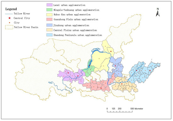
Figure 1.
Schematic diagram of the urban agglomeration in the Yellow River Basin (YRB).
3.2. Data Sources
The data sources included NTL data: DMSP-OLS and NPP/VIIRS. Statistical data: labor put, capital input, education development, and traffic level, in terms of city scale (72 cities in total). Descriptive information on the data sources is given in Table 1.

Table 1.
Description of the data sources.
DMSP-OLS, Defense Meteorological Satellite Program’s Operational Linescan System; NPP/VIIRS, National Polar-orbiting Partnership/Visible Infrared Imaging Radiometer Suite; GDP, gross domestic product.
Among them, the missing highway mileage of Xining city in Qinghai province, Wuzhong city in Ningxia Autonomous Region, Yinchuan city, and Shizuishan city was calculated by multiplying the highway mileage in the historical years by the estimated growth rate.
3.3. Night Light Datasets
The official website of the National Geophysical Data Center (NGDC) of the National Oceanic and Atmospheric Administration (NOAA) can download DMSP-OLS and NPP/VIIRS night light data for free. Among them, DMSP-OLS contained 6-generation satellite data that can be detected from 1992 to 2013. This paper selected DMSP-OLS night stable light data as the research basis. DMSP-OLS data have been widely used in many research fields due to its advantages, such as wide spatial coverage and long time span. However, there were two problems with this data. The first was the problem of pixel saturation in the center of the city, and the second was the lack of comparability between the pixels of the DMSP-OLS NTL data [55].
Compared with DMSP-OLS NTL data, the NPP/VIIRS sensor can detect weaker light, with higher temporal and spatial resolution. NPP/VIIRS NTL data did not have the “ceiling phenomenon” of pixels, but it did not remove the sporadic faint lights, such as flares, which will cause high image noise. At the same time, although the NPP/VIIRS NTL data were more time-sensitive monthly synthetic data, the time span was relatively short, only starting to save lighting image data in 2012; and only 2015 and 2016 provide annual synthetic data, and the rest were monthly. In order to overcome this interference, based on annual synthesis of the data, it was necessary to perform noise reduction processing and resampled the resolution to 1 km × 1 km so that it can be fused with DMSP-OLS NTL data to construct an NTL dataset with a large time span.
In order to obtain long-time series of NTL data to represent the level of economic development, the results of the literature [54,56] were applied, mainly including the following aspects. (1) Through mutual correction and fusion of DMSP-OLS NTL data, the problem of pixel saturation of DMSP-OLS data and lack of comparability of data pixels was solved. (2) In order to reduce the influence of noise, this paper took the stable bright element area of the 2016 annual synthetic data as the invariable area and makes stability corrections to the 2012–2018 data. (3) The last aspect is integrating these two datasets. Consequently, we produced the integrated NTL datasets (1995–2018); more details can be seen in Reference [54].
In the ArcGIS software environment, at the projection of Lambert Azimuthal Equal Area, the image was cut with the vector map mask of the urban agglomerations in the YRB in order to obtain the NTL image data of the corresponding year. The spatial resolution was 1 km × 1 km. In order to avoid the interference of the county area, the average light value for each county at night was employed to measure the economic development level for each county.
3.4. Research Methods
3.4.1. Spatial Autocorrelation Analysis
Spatial autocorrelation analysis can analyze the distribution characteristics and regular pattern of each economic attributes, and whether there are aggregation characteristics or interdependence.
- (1)
- Global spatial autocorrelation
Global Moran’s I was selected to test the overall spatial attribute of the economic development level for all counties in the urban agglomeration of the YRB. The specific calculation is as follows:
where and represent the economic development level of and counties, respectively; represents the number of counties; is the space weight matrix; and represents the surface distance between counties calculated by latitude and longitude. The value range of I is [−1, 1]; the closer to 1, the positive spatial correlation is significant; the closer to −1, the negative spatial correlation is significant. Equation (4) was used to conduct a statistical test on the Global Moran’s I results:
In the formula, represents the variance of Global Moran’s I. When is greater than the critical value 1.96 of normal distribution at the significant level of 0.05, it is considered that Global Moran’s I results are significant.
- (2)
- Local Getis-Ord G
The Local Getis-Ord G, also known as a hot-spot analysis, was used to generate the weight matrix with the spatial approach defined by distance, and its calculation formula is as follows:
The test of statistics is similar to the local Moran index, and its test value is as follows:
When the value of local Getis-Ord G is greater than the mathematical expectation and passes the hypothesis test, it shows that the value around the county is relatively high (higher than the average) and belongs to the spatial agglomeration of high value (hot spot). When the value of local Getis-Ord G is less than the mathematical expectation and passes the hypothesis test, it shows that the value around the county is relatively low (lower than the average) and belongs to the spatial clustering of low values (cold spot area). To further, identify whether there is a hot spot clustering location for regional economic attribute development in a small local area.
3.4.2. Standard Deviation and Coefficient of Variation
The sample standard deviation is usually used to reflect the dispersion degree of individuals in a group. The larger the sample standard deviation is, the greater the difference between most of the values and the average value will be, and vice versa, as shown in Equation (7):
The coefficient of variation is the ratio between the standard deviation of the original data and the average of the original data that also reflects the degree of data dispersion. As shown in Equation (8), it can eliminate the influence of measurement scale and dimension.
In the above two equations, is the economic development level of each county, is the number of counties in the YRB urban agglomerations, and is the average economic development level of all counties in the YRB urban agglomerations in 2018.
3.4.3. MGWR
Compared with the traditional classic GWR, MGWR mainly has the following three important improvements: The first is allowing each variable to have a different spatial smoothing level solves the shortcomings of the classic GWR model. Second, the specific bandwidth of each variable can be used as an indicator of the spatial scale of each spatial process. Third, the multi-bandwidth method produces a more realistic and useful spatial process model [22]. The calculation formula of the MGWR model is as shown in Equation (9):
where represents the bandwidth used by the regression coefficient of variable. Each regression coefficient of MGWR is obtained based on local regression, and the bandwidth is specific. This is the biggest difference from the classic GWR. In the classic GWR, all variables of have the same bandwidth. This paper uses Gaussian kernel function and Akaike information criterion (AIC) as the kernel function and bandwidth selection criterion of MGWR. The details of the process can be found in Fotheringham et al. (2017) [52] and Oshan, Li, Kang, Wolf, and Fotheringham (2019) [57].
In this article, all calibrations of the MGWR models were undertaken by MGWR2.2 software [57].
4. Results and Analysis
4.1. Spatio-Temporal Evolution Analysis
Using ArcGIS software and adopting the natural fracture method, economic development levels of the counties in 1992, 2005, and 2018 were divided into five grades: highest level, higher level, medium level, lower level, and lowest level (Figure 2).
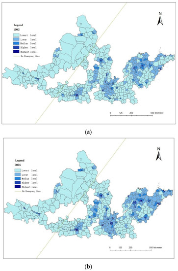
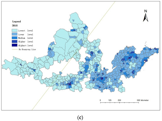
Figure 2.
Economic development levels of counties in seven urban agglomerations: (a) 1992, (b) 2005, and (c) 2018.
The overall economic development of counties in the urban agglomeration of the YRB is at a low and uneven level, representing a development trend of “low in the west, high in the east”. The number of counties belonging to the lower level is more as compared to the other levels. The number of highest and higher level counties is much less than that of the low and lower level counties. The overall development level of counties in the east of Hu Huanyong Line is comparatively higher than that in the west. In terms of time trend, the number of counties above the medium level is gradually increasing, while the number of counties at a low level is gradually decreasing. In addition, low-level counties are more concentrated in the urban agglomerations to the west of the Hu Huanyong Line, as compared to the other places, and their geographical location is closer to the provincial boundary with prominent characteristics of boundary effect.
Figure 3 shows the number of counties with the highest and higher levels corresponding to the seven urban agglomerations in the YRB in 1992, 2005, and 2018, respectively.
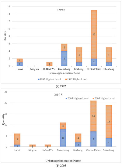
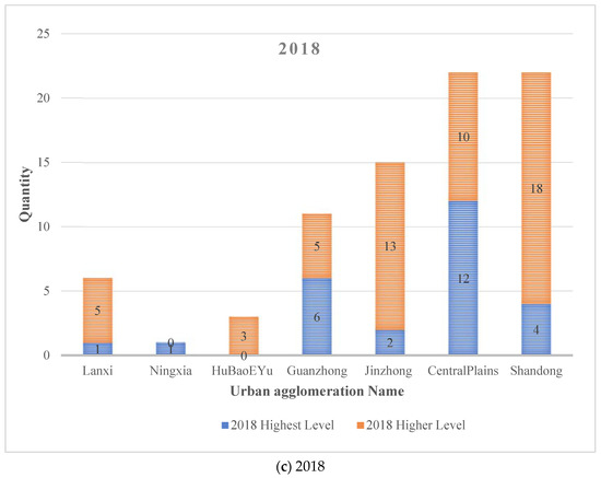
Figure 3.
The number of counties above the medium level in the seven urban agglomerations.
In 1992, the highest-level counties were mainly concentrated in the Central Plains urban agglomeration. In 2005, it was mainly concentrated in the Guanzhong Plain, Central Plains, and Shandong Peninsula urban agglomeration. In 2018, it was mainly concentrated in the Guanzhong Plain, Jinzhong, Central Plains, and Shandong Peninsula urban agglomeration. Although the number of counties in Lanxi, Ningxia Yanhuang, and Hubao Eyu urban agglomerations increased with time, the overall number is still small.
As shown in Figure 4, from 1992 to 2018, the standard deviation of the economic development level of counties in the urban agglomerations of the YRB has risen from 9.1876 to 24.6360, indicating that the economic development level of most the counties is still far from the medium development level. The coefficient of variation decreased from 1.4662 to 1.0325, indicating that the relative differences in the level of economic development of counties in the YRB are reduced to some extent, and the situation of economic development imbalance is alleviated.
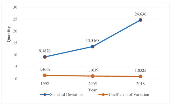
Figure 4.
Standard deviation and coefficient of variation of the economic development levels in the seven urban agglomerations.
4.2. Spatial Autocorrelation Analysis
4.2.1. Global Autocorrelation Analysis
Table 2 shows the global Moran’s I index of the average night light data for each county in the urban agglomeration of the YRB. The Z-value shows that the test results are significant, indicating that the night light data of counties in the urban agglomeration in the YRB have positive spatial autocorrelation. The Moran’s I index has been continuously improving from 1992 to 2018, indicating that the spatial correlation of counties in the urban agglomeration of the YRB has been increasing year by year. The overall Moran’s I index values are not high, which reflects the low spatial agglomeration degree of urban agglomeration in the YRB as a whole, and there is a need to strengthen the economic relations among the counties.
Table 2.
Overall Moran’s I index.
4.2.2. Local Cold and Hot Spots Analysis
Using ArcGIS software, according to the critical value of the corresponding Z-value under 5% and 10% confidence level, the local spatial correlation index of the respective economic development level in 1992, 2005, and 2018 was divided into five types of regions, as shown in Table 3.
Table 3.
Cold and hot spots partitioning.
By analyzing and comparing the changes of cold and hot spots (as shown in Figure 5), the clustering evolution pattern of the county economic space in the urban agglomeration of the YRB is further grasped.
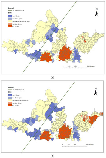
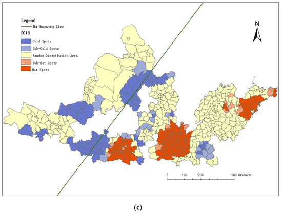
Figure 5.
Cold and hot spots of economic development: (a) 1992, (b) 2005, and (c) 2018.
Overall, the sub-hot spots and hot spots of county economic development in the urban agglomeration of the YRB are concentrated to the east of the Hu Huanyong Line, and the sub-cold spots and cold spots are mostly distributed in the urban agglomeration near and to the west of the Hu Huanyong Line. The imbalance pattern of “West-cold and East-hot” polarization is obvious.
From the perspective of geographical location, most of the sub-hot spots and hot spots are located in the central hinterland of urban agglomerations, mainly in Guanzhong, Central Plains, and Shandong Peninsula urban agglomerations.
The sub-cold spots and cold spots are mainly located at the junction of the urban agglomerations, far away from the counties of central cities. The shielding effect of the boundary makes their economic development level low, and they represent the characteristics of contiguous poverty. These spots are Longxi County, Wushan County, Qinzhou District, Maiji District, Feng County, etc., at the junction of the Lanxi and the Guanzhong Plain urban agglomerations, as well as the contiguous destitute areas that appeared in the Jinzhong urban agglomerations in 2018, including Xiangning County, Lingshi County, Huozhou City, Hongdong County, Xiangfen County, and Hancheng City.
- (1)
- Hot spots
As observed from the time trends of hot spots (Figure 6), the Jinzhong urban agglomeration and the Central Plains urban agglomeration have not changed much in the three time sections, while the Guanzhong Plain urban agglomeration shows a weak contraction trend. On the contrary, the Shandong Peninsula urban agglomeration shows a clear expansion trend with the passing of time, which means that the central city has a strong driving effect on the economic development of the hinterland counties, showing a spillover effect of “contiguous development”.
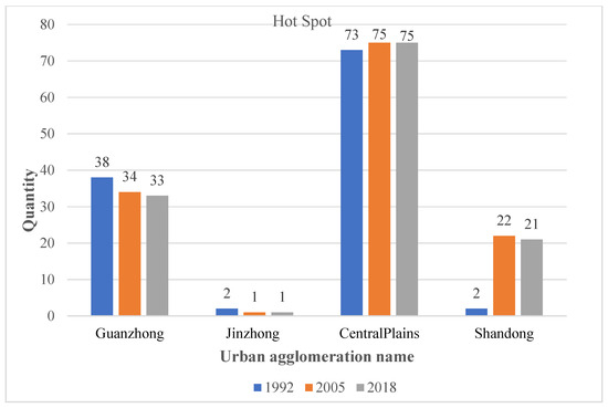
Figure 6.
Number of hot spots in 1992, 2005, and 2018.
The Central Plains, Guanzhong Plain, and the Shandong Peninsula urban agglomeration are all hot spots with high significance in the three time sections, indicating that these three places have a relatively high level of economic development compared to other regions and are the most dynamic core of the economic development of the urban agglomeration in the YRB.
- (2)
- Cold spots
As shown in Figure 7, except for the Central Plains and Shandong Peninsula urban agglomeration, the cold spot areas of other urban agglomerations showed an increasing trend with time. The number of cold spot counties at the junction of the Central Plains and the Shandong Peninsula decreased from 14 in 1992 to 10 in 2005 and to 3 in 2018.
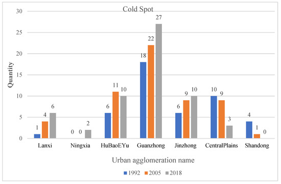
Figure 7.
Number of cold spots in 1992, 2005, and 2018.
4.2.3. Analysis of Influencing Factors
- (1)
- Model selection
The MGWR was more suitable to analyze the influencing factors of the economic development in the seven urban agglomerations of the YRB, because it not only allowed the parameter estimates to vary over space, but also produced individual optimal bandwidths for the conditional relationships between the response variable and each predictor variable, which allowed the spatial variation of different processes to be modeled at different spatial scales. Table 4 shows that the R2 and the adjusted R2 of the MGWR model were both higher, and the AIC value was lower than those of classic GWR model, indicating that the fitting performance of the MGWR model was better.
Table 4.
Model index of geographically weighted regression (GWR) and multi-scale GWR (MGWR) model.
- (2)
- Spatial Heterogeneity Regression Analysis
In order to maintain the integrity of statistical data to the greatest extent, this study took cities in the YRB urban agglomeration as the scale to study the different influences of various influencing factors on their economic development level and selected 2018 with good timeliness as the key year for research. The NTL data at the municipal scale representing the economic development level were the explained variable, and labor input, capital input, government force, traffic level, education development, medical level, and import and export as the explanatory variables.
As can be seen from Table 5, MGWR could directly reflect the differential action scales of different variables, while GWR could only reflect the average of the action scales of various variables.
Table 5.
Bandwidth comparison between MGWR and GWR.
In the MGWR regression results, labor input, government force, education development, import and export, and the regression coefficients of four variables were overall significant. The regression coefficients of capital input, traffic level and medical level were not significant. The statistical description of each coefficient of MGWR was shown in Table 6.
Table 6.
Statistical description of MGWR coefficient.
The spatial distribution of the coefficients of the four significant indicators was shown in Figure 8. Figure 8 used the natural fracture method to divide the impact of (a) labor input, (b) government force, (c) education development, and (d) import and export on the level of economic development in 2018.
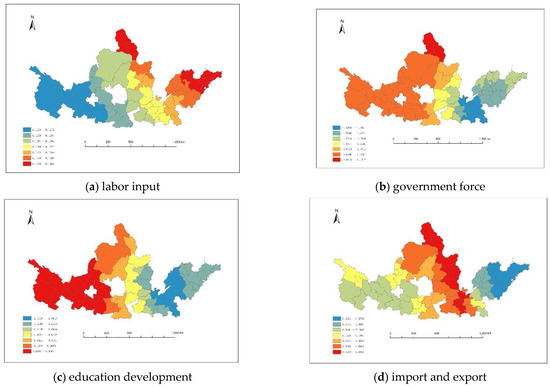
Figure 8.
Spatial differentiation of regression coefficients: (a) labor input, (b) government force, (c) education development, (d) import and export.
Labor input had a significant positive impact, as shown in Figure 8a. The impact of labor input had the characteristics of “polarization”. High values were mainly concentrated in the eastern part of the Hubao Eyu urban agglomeration, the northeast of the Jinzhong urban agglomeration, the eastern part of the Central Plains urban agglomeration and Shandong Peninsula urban agglomeration. The low values were mainly concentrated in Lanxi, Ningxia Yanhuang, and Guanzhong Plain urban agglomeration. The labor input coefficient ranged from 0.1271 to 0.1456, with a mean value of 0.133 and a standard deviation of 0.05. The maximum value was Weihai City in Shandong Peninsula urban agglomeration, 0.1455, and the minimum value was 0.1271 in the Huangnan Tibetan Autonomous Region in Lanxi urban agglomeration. From the point of view of the absolute value of the coefficient, the intensity of its influence was greater among all variables.
The government force had a significant and negative impact on the level of economic development, as shown in Figure 8b. Contrary to the influence of labor input, the influence coefficient of government force was “high in the west and low in the east”. The high values were mainly concentrated in Lanxi, Ningxia Yanhuang, Hubao Eyu, Guanzhong Plain urban agglomeration, and the northwestern part of Jinzhong urban agglomeration. The low values were mainly concentrated in the eastern part of Central Plains urban agglomeration and Shandong Peninsula urban agglomeration. The government force coefficient ranged from −0.1301 to −0.1547, with a mean value of −0.850 and a standard deviation of 0.398. The maximum value was Baotou City (−0.154676) in Hubao Eyu urban agglomeration, and the minimum value was Zhoukou City (−1.3009) in Central Plains urban agglomeration. From the point of view of the absolute value of the coefficient, the intensity of its influence was greater among all variables.
Education development reflected the duality of its impact on economic development, as shown in Figure 8c. The regions that reflected the positive impact of education development on the level of economic development were Lanxi; Ningxia Yanhuang; and Qingyang City, Pingliang City, Tianshui City, and Baoji City in the Guanzhong Plain urban agglomeration. Moreover, it had a negative impact on other regions. The value range of the education development coefficient was −1.4328~0.0984, the mean was −0.769, and the standard deviation was 0.636. The impact of education development on the level of economic development spaned a wide range. The maximum value was 0.0984 in Dingxi City in Lanxi urban agglomeration, and the minimum value was −1.4328 in Liaocheng City in Shandong Peninsula urban agglomeration.
Import and export had a significant positive impact on the development of the economic level, as shown in Figure 8d. High values were concentrated in Hubao Eyu, Jinzhong, and Central Plains urban agglomeration. Low values were concentrated in Shandong Peninsula, Lanxi urban agglomeration, and the western part of the Guanzhong Plain urban agglomeration. The import and export coefficient ranged from 0.2261 to 0.6988, with a mean value of 0.444 and a standard deviation of 0.115. It was the smallest span of regional differences among the four significant impact indicators. The maximum value was the Baotou City of Hubao Eyu urban agglomeration, which was 0.6988. The minimum value was the Weihai City in Shandong Peninsula urban agglomeration, which was 0.2261. From the perspective of the absolute value of the import and export coefficient, import and export had a relatively small impact on the level of economic development.
5. Discussion
The level of economic development was generally considered to be characterized by GDP. However, the calculation of GDP was based on various statistical data and statistical reports, and its authenticity or accuracy had always been questioned. The accuracy of GDP, especially in economically underdeveloped areas, had a larger gap than economically developed areas. Secondly, GDP was limited by statistical administrative units and lacks effective and accurate spatial location information, which was not conducive to small-scale regional economic development level research, such as the county level. In order to be more objective and to achieve the economic development level of the seven urban agglomerations in the YRB on a smaller scale, NTL datasets closely related to human activities were used as a substitute variable for the economic development level.
The most common DMSP-OLS or NPP/VIIRS NTL dataset had problems, such as time span. DMSP-OLS can be detected from 1992 to 2013, while NPP/VIIRS has only been detected since 2012. In order to study the level of economic development over a long period, it was necessary to effectively integrate the two types of NTL datasets. Using the team’s existing results, the integrated NTL dataset can be directly used to characterize the economic development level in the YRB, which can achieve a more effective analysis of spatial–temporal evolution over a longer span of time and on a smaller scale.
In the analysis of the spatial–temporal evolution of the economic development level at the county scale of the seven urban agglomerations in the YRB, it was found that the overall development level of the YRB is “low in the west and high in the east” (Figure 2). The urban agglomeration where counties above the medium level were concentrated had changed from the Central Plains urban agglomeration (1992, Figure 3a) to the Guanzhong Plain, Central Plains, and Shandong Peninsula urban agglomerations (2005, Figure 3b), and finally to the Guanzhong Plain, Jinzhong, Central Plains, and Shandong Peninsula urban agglomeration (2018, Figure 3c). The difference in the overall economic development level of the seven urban agglomerations in the YRB was analyzed by using the standard deviation and the coefficient of variation. Although the relative difference in economic development level of each urban agglomeration was decreasing over the years, the economic development level of most counties was still below the medium level (Figure 4).
In the analysis of the spatial autocorrelation of the economic development levels of the seven urban agglomerations at the county level, the global Moran’s I index showed that, although the economic spatial correlation of the counties in the urban agglomerations has increased year by year, the degree of spatial agglomeration was still low (Table 2). Analysis of local cold and hot spots showed that the economic development level of the seven urban agglomerations was “cold in the west and hot in the east”. Most of the secondary hot spots and hot spots were located in the central hinterland of the urban agglomeration, and the secondary cold spots and cold spots were located at the boundary of the urban agglomeration (Figure 5). The hot spots are mainly concentrated in the Central Plains, Guanzhong Plain and Shandong Peninsula urban agglomeration. The Shandong Peninsula urban agglomeration showed a trend of “contiguous overflow” (Figure 6). Except for the Central Plains and Shandong Peninsula urban agglomeration, the cold spots in other urban agglomerations showed the increasing trend year by year (Figure 7).
All indicators in Table 4 showed that the fitting performance of MGWR was better than that of the GWR model. Moreover, MGWR provided different bandwidth for different variables (Table 5). It was more appropriate to choose the MGWR model to analyze the influencing factors of the level of economic development. Labor input had positive impact on the level of economic development, and its spatial distribution was “low west and high east” (Figure 8a). Government force had negative impact. Moreover, the spatial distribution of government force was opposite to that of labor input, which was “high west and low east” (Figure 8b). The education development had both positive and negative effects, and the positive effects were concentrated in the west of the YRB. (Figure 8c). The import and export had positive impact on the level of economic development, and its spatial distribution was “high in the middle and low on the sides” (Figure 8d).
6. Conclusions and Suggestions
In order to obtain an alternative variable of the economic development levels with a long sequence and strong timeliness, this paper studied the economic development differences and spatial–temporal evolution rules of seven urban agglomerations in the YRB, at the county scale, based on the integrated DMSP-OLS and NPP/VIIRS NTL datasets. The results showed that the spatial pattern of its economic development presents an unbalanced trend of “low west and high east”. The “pyramid” level of economic development had obvious characteristics. In addition, the “contiguous extreme poverty” effect was obvious.
The global Moran’s I index showed that, although the spatial correlation of all counties in the YRB had been strengthened year by year, the overall degree of agglomeration was still not that high. Therefore, in future policymaking, policy makers should consider strengthening the intensity of economic ties between counties. The local Getis-Ord G showed that the Guanzhong Plain, Central Plains, and Shandong Peninsula urban agglomerations with concentrated hot spots and their central cities had a strong driving ability to the surrounding areas. Cold-spot areas, such as the counties adjacent to the Central Plains and Shandong urban agglomerations, showed a clear decreasing trend over time, indicating that the central cities of the two urban agglomerations had a good synergistic development effect on the economic development of the county near the provincial boundary. However, most cold spots still lacked connections with central cities and thus failed to establish a good synergy effect and present the characteristics of “contiguous poverty”. In future policy formulations, in addition to focusing on the economically active core areas of the Central Plains, Guanzhong Plain, and Shandong Peninsula urban agglomeration, more attention should be paid to the concentration of cold spots and the “contiguous poverty” areas. These areas were the key to attention and support area.
The results of the MGWR showed that labor input and import and export had a positive impact on the economic development level for each urban agglomeration, government force had a negative impact, and education showed both positive and negative polarization on economic development.
The regression coefficient of labor input showed that the marginal output of labor in the east was higher than that in the west, possibly because the technology level and high-tech industries in the east are relatively developed and concentrated, while the industries in the west were mostly low-value-added agricultural and resource-based. The employment quality of the local labor force should be improved in western urban agglomerations with a low marginal output of labor force. The first step is to support and build qualified business incubation bases, actively develop labor-intensive industries, and expand nearby employment space for labor. The second step is to strengthen labor skills training, guide and support enterprises to carry out order-oriented training, and guide the people to stay and build the local area.
The negative impact of the government force indicated that the national policy was not strong enough to cover the urban agglomerations in the YRB. In the future development, the government could pay more attention and support to the development of the urban agglomerations in the YRB. For example, based on the different natural resources, cultural and historical advantages of different urban agglomerations promote the construction and development of characteristic towns, characteristic industries, and characteristic parks.
The relatively low level of economic development in regions where the education development produced positive impact indicated that the level of education in these regions was relatively backward and the momentum of education development was insufficient. The level of economic development in the regions with negative correlations was relatively high, which implied that there was a serious loss of high-level talents in these regions. In future policy formulation, the education level of urban agglomerations should be improved, and the talent drop policy should be strengthened. Optimize the layout of primary and secondary schools, accelerate the popularization of high school education, and promote the balanced development of education among urban agglomerations. Improve the quality of secondary and higher technical schools, and cultivate more technical and technical talents that meet the needs of social development. Strengthen and integrate knowledge and the Internet and enhance openness and sharing. Optimize the talent landing policy, give higher treatment to scarce talents, and avoid the loss of urban talent resources.
Import and export had a positive impact on all urban agglomerations, and the high values were concentrated in the Hubao Eyu, Jinzhong, and Central Plains urban agglomerations. Overall, the impact of import and export on all urban agglomerations was not very different. In the future, more attention should be paid to the import and export of specialty products in urban agglomerations to increase capital circulation. For example, vigorously promote the construction of high-grade highways and railways in the various urban agglomerations along the YRB. For the interior of each urban agglomeration, it is necessary to strengthen the transportation links between the central city and the hinterland and border cities, and provide a closer transportation link between them on a hardware basis.
Author Contributions
J.W. and H.L. (Haibin Liu) conceived and designed the study. Q.L. and H.L. (Hao Liu) processed the data and performed analysis. Y.S. and H.H. contributed to the interpretation of the results. J.W. and D.P. wrote the paper. All authors reviewed and edited the draft, approved the submitted manuscript, and agreed to be listed and accepted the version for publication. All authors have read and agreed to the published version of the manuscript.
Funding
This research was funded by “The Fundamental Research Funds for the Central Universities” grant number 2020YJSGL01.
Institutional Review Board Statement
Not applicable.
Data Availability Statement
Data sharing not applicable.
Conflicts of Interest
The authors declare no conflict of interest.
References
- Zhang, P.; Pang, B.; Li, Y.; He, J.; Hong, X.; Qin, C.; Zheng, H. Analyzing spatial disparities of economic development in Yellow River Basin, China. Geo J. 2018, 84, 303–320. [Google Scholar] [CrossRef]
- Liu, K.; Qiao, Y.; Shi, T.; Zhou, Q. Study on coupling coordination and spatiotemporal heterogeneity between economic development and ecological environment of cities along the Yellow River Basin. Environ. Sci. Pollut. Res. 2021, 28, 6898–6912. [Google Scholar] [CrossRef]
- Wohlfart, C.; Liu, G.; Huang, C.; Kuenzer, C. A River Basin over the Course of Time: Multi-Temporal Analyses of Land Surface Dynamics in the Yellow River Basin (China) Based on Medium Resolution Remote Sensing Data. Remote Sens. 2016, 8, 186. [Google Scholar] [CrossRef]
- Chen, Y.; Zhu, M.; Lu, J.; Zhou, Q.; Ma, W. Evaluation of ecological city and analysis of obstacle factors under the background of high-quality development: Taking cities in the Yellow River Basin as examples. Ecol. Indic. 2020, 118, 106771. [Google Scholar] [CrossRef]
- Lan, F.; Da, H.; Wen, H.; Wang, Y. Spatial Structure Evolution of Urban Agglomerations and Its Driving Factors in Mainland China: From the Monocentric to the Polycentric Dimension. Sustainability 2019, 11, 610. [Google Scholar] [CrossRef]
- He, Y.; Zhou, G.; Tang, C.; Fan, S.; Guo, X. The spatial organization pattern of urban-rural integration in urban agglomerations in China: An agglomeration-diffusion analysis of the population and firms. Habitat Int. 2019, 87, 54–65. [Google Scholar] [CrossRef]
- Gottmann, J. Megalopolis or the urbanization of the northeastern seaboard. Econ. Geogr. 1957, 33, 189–200. [Google Scholar] [CrossRef]
- Fang, C.; Yu, D. Urban agglomeration: An evolving concept of an emerging phenomenon. Landsc. Urban Plan. 2017, 162, 126–136. [Google Scholar] [CrossRef]
- Yuan, W.; Li, J.; Meng, L.; Qin, X.; Qi, X. Measuring the area green efficiency and the influencing factors in urban agglomeration. J. Clean. Prod. 2019, 241, 118092. [Google Scholar] [CrossRef]
- Gu, C. Study on urban agglomeration: Progress and prospects. Geogr. Res. 2011, 30, 771–784. [Google Scholar] [CrossRef]
- Xu, C.; Wang, S.; Zhou, Y.; Wang, L.; Liu, W. A Comprehensive Quantitative Evaluation of New Sustainable Urbanization Level in 20 Chinese Urban Agglomerations. Sustainability 2016, 8, 91. [Google Scholar] [CrossRef]
- Costanza, R.; Kubiszewski, I.; Giovannini, E.; Lovins, H.; McGlade, J.; Pickett, K.E.; Ragnarsdóttir, K.V.; Roberts, D.; De Vogli, R.; Wilkinson, R.G. Development: Time to leave GDP behind. Nat. Cell Biol. 2014, 505, 283–285. [Google Scholar] [CrossRef] [PubMed]
- Henderson, J.V.; Storeygard, A.; Weil, D.N. Measuring economic growth from outer space: The National Bureau of Economic Research. Am. Econ. Rev. 2012, 102, 994–1028. [Google Scholar] [CrossRef] [PubMed]
- Rawski, T.G. What is happening to China’s GDP statistics? China Econ. Rev. 2001, 12, 347–354. [Google Scholar] [CrossRef]
- Dai, Z.; Hu, Y.; Zhao, G. The Suitability of Different Nighttime Light Data for GDP Estimation at Different Spatial Scales and Regional Levels. Sustainability 2017, 9, 305. [Google Scholar] [CrossRef]
- Hu, Y.; Peng, J.; Liu, Y.; Du, Y.; Li, H.; Wu, J. Mapping Development Pattern in Beijing-Tianjin-Hebei Urban Agglomeration Using DMSP/OLS Nighttime Light Data. Remote Sens. 2017, 9, 760. [Google Scholar] [CrossRef]
- Shi, K.F.; Yu, B.L.; Huang, Y.X.; Hu, Y.J.; Yin, B.; Chen, Z.Q.; Chen, L.J.; Wu, J.P. Evaluating the Ability of NPP-VIIRS Nighttime Light Data to Estimate the Gross Domestic Product and the Electric Power Consumption of China at Multiple Scales: A Comparison with DMSP-OLS Data. Remote Sens. 2014, 6, 1705–1724. [Google Scholar] [CrossRef]
- Jing, X.; Shao, X.; Cao, C.; Fu, X.; Yan, L. Comparison between the Suomi-NPP Day-Night Band and DMSP-OLS for Correlating Socio-Economic Variables at the Provincial Level in China. Remote Sens. 2015, 8, 17. [Google Scholar] [CrossRef]
- Wang, J.; Liu, H.; Liu, H.; Huang, H. Spatiotemporal evolution of multiscale urbanization level in the Beijing-Tianjin-Hebei Region using the integration of DMSP/OLS and NPP/VIIRS night light datasets. Sustainability 2021, 13, 2000. [Google Scholar] [CrossRef]
- Huang, Q.; Yang, Y.; Li, Y.; Gao, B. A Simulation Study on the Urban Population of China Based on Nighttime Light Data Acquired from DMSP/OLS. Sustainability 2016, 8, 521. [Google Scholar] [CrossRef]
- Goodchild, M.F. Models of Scale and Scales of Modelling. In Modelling Scale in Geographical Information Science; John Wiley & Sons, Ltd.: Hoboken, NJ, USA, 2001; pp. 3–10. [Google Scholar]
- Shen, T.; Yu, H.; Zhou, L.; Gu, H.; He, H. On Hedonic Price of Second-Hand Houses in Beijing Based on Multi-Scale Geograph-ically Weighted Regression: Scale Law of Spatial Heterogeneity. Econ. Geogr. 2020, 40, 75–83. [Google Scholar] [CrossRef]
- Meng, D.Y.; Li, X.J.; Lu, Y.Q. Evolvement of Spatial Pattern of Urban Economic Development in Yangtze River Delta. Econ. Geogr. 2014, 34, 50–57. [Google Scholar] [CrossRef]
- Xu, J.H.; Lu, F.; Su, F.L.; Lu, Y. Spatial and temporal scale analysis on the regional economic disparities in China. Geogr. Res. 2005, 24, 57–68. [Google Scholar] [CrossRef]
- Chen, Z. Regional development difference from the south to the north ineast and middle China. Geogr. Res. 1999, 80–87. [Google Scholar] [CrossRef]
- Rozelle, S. Rural Industrialization and Increasing Inequality: Emerging Patterns in China’s Reforming Economy. J. Comp. Econ. 1994, 19, 362–391. [Google Scholar] [CrossRef]
- Wang, Y.; Ma, F. Research on Regional Economic Disparity in Yellow River Basin. J. Xi’an Univ. Financ. Econ. 2008, 2, 23–26. [Google Scholar] [CrossRef]
- Sang, Q.; Zhang, P.Y.; Gao, X.N.; Xin, X. Spatio-temperal Characteristics of sparity of Counties Comprehensive Development Level in Central Liaoning Urban Agglomeration. Sci. Geogr. Sin. 2008, 2, 150–155. [Google Scholar] [CrossRef]
- Ma, J.; Wang, J.; Szmedra, P. Economic efficiency and its influencing factors on urban agglomeration—An analysis based on China’s top 10 urban agglomerations. Sustainability 2019, 11, 5380. [Google Scholar] [CrossRef]
- Xue, B. Analysis of Spatial Pattern Evolution of Economy in Central Plains Economic Region. Econ. Geogr. 2013, 33, 15–20. [Google Scholar] [CrossRef]
- Hu, Z.; Ou, X. Analysis of Regional Inequality in Jiangsu Province by Multi-target Measure Based on Theil Index. Econ. Geogr. 2013, 27, 719–724. [Google Scholar] [CrossRef]
- Zhang, X.; Wang, M. Spatial Analysis of County Economic Differences and Temporal-Spatial Evolution of Guan-Zhong-TianShui Economic Zone. Econ. Geogr. 2011, 24, 889–906. [Google Scholar] [CrossRef]
- Zhou, G.; Xia, X. The Convergence and the Impact Factors of Regional Economic Growth in China—An Empirical Analysis of The Yellow River Basin. Stat. Res. 2008, 11. [Google Scholar] [CrossRef]
- Liu, Z.; Yang, Q. Research on the spatial polarization and its influencing factors in Shandong Peninsula urban agglomerations regions. Resour. Environ. Yangtze Basin 2011, 20, 790–795. [Google Scholar] [CrossRef]
- Qin, C.; Zhou, E. The Patterns of Spatial Differentiation of Economies in Yellow River Basin. J. Henan Univ. (Nat. Sci.) 2010, 40, 40–44. [Google Scholar] [CrossRef]
- Zhang, Q.; Seto, K.C. Mapping urbanization dynamics at regional and global scales using multi-temporal DMSP/OLS nighttime light data. Remote Sens. Environ. 2011, 115, 2320–2329. [Google Scholar] [CrossRef]
- Zhuo, L.; Ichinose, T.; Zheng, J.; Chen, J.; Shi, P.J.; Li, X. Modelling the population density of China at the pixel level based on DMSP/OLS non-radiance-calibrated night-time light images. Int. J. Remote Sens. 2009, 30, 1003–1018. [Google Scholar] [CrossRef]
- Yi, K.; Tani, H.; Li, Q.; Zhang, J.; Guo, M.; Bao, Y.; Wang, X.; Li, J. Mapping and evaluating the urbanization process in northeast China using DMSP/OLS nighttime light data. Sensors 2014, 14, 3207–3226. [Google Scholar] [CrossRef] [PubMed]
- Zhou, N.; Hubacek, K.; Roberts, M. Analysis of spatial patterns of urban growth across South Asia using DMSP-OLS nighttime lights data. Appl. Geogr. 2015, 63, 292–303. [Google Scholar] [CrossRef]
- Sutton, P.; Roberts, D.; Elvidge, C.; Meij, H. A comparison of nighttime satellite imagery and population density for the continental United States. Photogramm. Eng. Remote Sens. 1997, 63, 1303–1313. [Google Scholar]
- Lo, C. Modeling the population of China using DMSP operational linescan system nighttime data. Photogramm. Eng. Remote Sens. 2001, 67, 1037–1047. [Google Scholar]
- Tan, M.; Li, X.; Li, S.; Xin, L.; Wang, X.; Li, Q.; Li, W.; Li, Y.; Xiang, W. Modeling population density based on nighttime light images and land use data in China. Appl. Geogr. 2018, 90, 239–247. [Google Scholar] [CrossRef]
- Elvidge, C.D.; Baugh, K.E.; Kihn, E.A.; Kroehl, H.W.; Davis, E.R.; Davis, C.W. Relation between satellite observed visible-near infrared emissions, population, economic activity and electric power consumption. Int. J. Remote Sens. 1997, 18, 1373–1379. [Google Scholar] [CrossRef]
- Amaral, S.; Câmara, G.; Monteiro, A.M.V.; Quintanilha, J.A.; Elvidge, C.D. Estimating population and energy consumption in Brazilian Amazonia using DMSP night-time satellite data. Comput. Environ. Urban Syst. 2005, 29, 179–195. [Google Scholar] [CrossRef]
- Chand, T.R.K.; Badarinath, K.V.S.; Elvidge, C.D.; Tuttle, B.T. Spatial characterization of electrical power consumption patterns over India using temporal DMSP-OLS night-time satellite data. Int. J. Remote Sens. 2009, 30, 647–661. [Google Scholar] [CrossRef]
- Jiansheng, W.; Yan, N.; Jian, P.; Zheng, W.A.N.G.; Xiulan, H.U.A.N.G. Research on energy consumption dynamic among prefecture-level cities in China based on DMSP/OLS nighttime light. Geogr. Res. 2014, 33, 625–634. [Google Scholar] [CrossRef]
- Fang-dao, Q.I.U.; Lian-jun, T.O.N.G.; Chuan-geng, Z.H.U.; Ru-shu, Y.A.N.G. Spatio-temporal pattern and driving mechanism of economic development discrepancy in provincial border-regions: A case study of Huaihai economic zone. Geogr. Res. 2009, 28, 451–463. [Google Scholar] [CrossRef]
- Lazar, M. Shedding light on the global distribution of economic activity. Open Geogr. J. 2010, 3, 147–160. [Google Scholar] [CrossRef]
- Fu, H.; Shao, Z.; Fu, P.; Cheng, Q. The Dynamic Analysis between Urban Nighttime Economy and Urbanization Using the DMSP/OLS Nighttime Light Data in China from 1992 to 2012. Remote Sens. 2017, 9, 416. [Google Scholar] [CrossRef]
- Xu, K.; Chen, F.; Liu, X. The truth of China economic growth: Evidence from global night-time light data. Econ. Res. J. 2015, 9, 17–29. [Google Scholar]
- Fotheringham, A.S.; Brunsdon, C.; Charlton, M. Geographically Weighted Regression: The Analysis of Spatially Varying Relationships; John Wiley & Sons: Hoboken, NJ, USA, 2003. [Google Scholar]
- Fotheringham, A.S.; Yang, W.; Kang, W. Multiscale geographically weighted regression (MGWR). Ann. Am. Assoc. Geogr. 2017, 107, 1247–1265. [Google Scholar] [CrossRef]
- Yu, H.; Fotheringham, A.S.; Li, Z.; Oshan, T.; Kang, W.; Wolf, L.J. Inference in Multiscale Geographically Weighted Regression. Geogr. Anal. 2020, 52, 87–106. [Google Scholar] [CrossRef]
- Lv, Q.; Liu, H.; Wang, J.; Liu, H.; Shang, Y. Multiscale analysis on spatiotemporal dynamics of energy consumption CO2 emissions in China: Utilizing the integrated of DMSP-OLS and NPP-VIIRS nighttime light datasets. Sci. Total. Environ. 2020, 703, 134394. [Google Scholar] [CrossRef] [PubMed]
- Yue, Y.; Tian, L.; Yue, Q.; Wang, Z. Spatiotemporal Variations in Energy Consumption and Their Influencing Factors in China Based on the Integration of the DMSP-OLS and NPP-VIIRS Nighttime Light Datasets. Remote Sens. 2020, 12, 1151. [Google Scholar] [CrossRef]
- Liu, Z.; He, C.; Zhang, Q.; Huang, Q.; Yang, Y. Extracting the dynamics of urban expansion in China using DMSP-OLS nighttime light data from 1992 to 2008. Landsc. Urban Plan. 2012, 106, 62–72. [Google Scholar] [CrossRef]
- Oshan, T.M.; Li, Z.; Kang, W.; Wolf, L.J.; Fotheringham, A.S. mgwr: A Python Implementation of Multiscale Geographically Weighted Regression for Investigating Process Spatial Heterogeneity and Scale. ISPRS Int. J. Geo-Inf. 2019, 8, 269. [Google Scholar] [CrossRef]
Publisher’s Note: MDPI stays neutral with regard to jurisdictional claims in published maps and institutional affiliations. |
© 2021 by the authors. Licensee MDPI, Basel, Switzerland. This article is an open access article distributed under the terms and conditions of the Creative Commons Attribution (CC BY) license (https://creativecommons.org/licenses/by/4.0/).