1. Introduction
Greenhouse gass (GHG) emissions produced during energy generation constitute one of the main causes of anthropogenic climate change [
1]. Due to that, a reduction of greenhouse emissions necessarily requires an increase in the share of renewable energy and a progressive energy transition. Because renewable energy generation fluctuates in time due to climate variability, the characterisation of the future climate is crucial for a transition towards renewable energy [
2,
3,
4,
5,
6]. This aspect is particularly important in islands, as the insular nature of which makes them totally, or partially, dependent on energy imports. Therefore, a transition towards renewable energies intended to lower GHG emissions and reduce energy dependence necessarily requires a good characterisation of present and future climate variability, especially when long-term investments are planned. Climate models are the only way to perform climate projections and study renewable energy resources in the future. In particular, regional climate models, which attain fine horizontal resolution at the expense of a smaller domain than that from global climate models, are the most suitable tool for regional purposes and particularly for islands [
7].
Solar PV (photovoltaic) and wind energy are presently, and likely in the future, the main technologies in the deployment of renewable energies due to their reduced cost and technological maturity [
8]. Because of that, the interest and amount of research on PV and wind energy using regional climate models has increased rapidly [
5,
9,
10,
11,
12,
13,
14,
15,
16,
17]. Additionally, offshore wind technologies are growing fast and they are expected to become one of the main sources of electricity generation due to the reduced time variability of offshore winds (compared to onshore winds) and to their high capacity factor [
18,
19,
20]. The technological development of the offshore wind will be specially interesting for islands, since suitable onshore locations are scarce due to space limitations. Likewise, offshore PV energy has advantages for islands or countries with restrictions in space for the installation, besides the increased performance due to the cooling effect of the water on PV cells [
21]. Although in a less mature stage of development, the installation of floating PV panels has been already tested over sea waters next to Malta [
22] and one offshore PV farm is already operating near the coast of the Netherlands [
23], an area characterised by high ocean waves.
Regarding that aspect, there is growing interest in the combination of different types of offshore renewable energy sources (including wind and solar) in the same location. On the one hand, because of the complementarity in time of the resources, which made the combined output more stable. On the other hand, it could be a reduction in costs, due to the simplification of the installations that could be partly shared [
24]. An example is that there are now projects for designing a floating offshore platform integrating wind, PV and wave energy for use on islands [
25]. This project will develop roadmaps for its deployment in three case study islands, among them the Canary Islands [
26]. Among the European islands, the Canary Islands, which constitute an integral part of Spain, located about 100 km off the African coast and comprise seven islands of volcanic origin, stand out as an excellent region to investigate for several reasons. First, they are characterised by a great solar resource potential, with a summer maximum that presently produces more than 22,000 MWh [
13] on the archipelago. In addition, the presence of persistent winds (i.e., trade winds and the Canary Low-Level Jet), which presently ensure a sustained wind energy productivity over time, much higher than in other regions such as the Mediterranean Islands [
27,
28,
29].
Regarding future projections, climate model simulations with the RCP4.5 and RCP8.5 scenarios indicate that future annual-mean changes in irradiation will not be relevant, whilst PV potential is expected to increase in winter due to a reduction of cloud cover and to decrease in summer in response to a temperature rise [
13]. In addition to this, previous modelling works have found a slight increase in the wind energy in the offshore area near the Canary Islands for the RCP8.5 and RCP4.5 scenarios for the 2070–2099 time period [
14,
15]. In spite of the promising climate characteristics of the Canary Islands for renewable energy generation, these are highly dependent on energy imports (e.g., oil) and the electricity network is not connected to the mainland grid. These problems are exacerbated by the fact that islands are not interconnected with each other (with the exception of Lanzarote and Fuerteventura). Only recently, the first large offshore wind power farm in Spain has been projected in the Canary Islands Special Zone [
30], which represents an important step towards the energy transition.
The aim of this work is to evaluate renewable resources in present and future climate (2046–2065 and 2081–2100), and their potential changes with respect to present conditions making use of regional climate model simulations from the MENA-CORDEX dataset [
31] in the Canary Islands and the sorrounding regions. In addition to the analysis of photovoltaic and wind productivity, variability of the resources is also studied through the concept of energy droughts [
29,
32], which is not as frequently analyzed as mean resource values. Energy productivity droughts can be regarded as low-productivity periods and are therefore an indicator of productivity variability. In addition, a complementarity analysis of solar and wind resources is made through a sensitivity test that provides the optimum share of each technology to reduce total power variability at each location. The relevance of this work is not only to show future evolution of renewable resources, but also to provide an assessment on their variability and complementarity in future conditions. This paper is structured as follows. In
Section 2 the methodology is described. In
Section 3 the most relevant results are presented and discussed. Conclusions are presented in
Section 4.
2. Methodology
In this work we make use of variables from a set of simulations from regional climate models of the MENA-CORDEX dataset. These simulations are used to estimate present values and future changes in energy productivity (wind and solar), variability (estimated through the so-called energy droughts and its frequency and persistence conditions) and complementarity between sources. The chosen models are shown in
Table 1.
Wind and solar productivity are defined as the normalised series of power generation, that is to say the produced energy divided by the capacity installed and is given in kWh/kW. Variability is assessed through energy drought days and the persistence of these days (i.e., number of consecutive drought days, cdd). Complementarity assessment is made considering a energy coming from PV and wind only and an optimization criterion is used to obtain the PV and wind share that minimizes variability.
All these variables are computed for a control time period (1986–2005), as well as for the mid and final stages of the 21st century (i.e., 2046–2065 and 2081–2100, respectively). To study future climate changes we use data from simulations forced with the RCP2.6 and RCP8.5 emission scenarios.
As to marine energy sources, we take into account not only offshore wind but also offshore solar PV energy, in addition to onshore resources. On the one hand, this is done for consistency reasons as we consider a combined PV-wind energy indicator, but also because of the growing interest in offshore solar energy. The considered domain (25.75° to 31.25° N, −10.25° to −11.75° W) for the analysis is far from the islands coast, will allow us to get better insights from the climate variables patterns and its evolution.
2.1. Models
The MENA-CORDEX dataset comprises a set of simulations of 0.44° horizontal resolution made with several regional climate models (RCMs) driven by different global climate models (GCMs). Only one RCMs in the MENA-CORDEX simulation list has available the RCP2.6 scenario. In this work, the selected simulations consist of this RCM (SMHI-RCA4) nested in three different GCMs (EC-EARTH-ICHEC, CNRM-CM5, GFDL-ESM2M2) for evaluation of the present period and two different scenarios: RCP2.6 and RCP8.5. The results presented are the averaged results of three simulations for the control period and the RCP8.5 scenario, whereas only one simulation is available for the RCP2.6. When differences between scenarios and control are presented, only the control period of the EC-EARTH-ICHEC is used for RCP2.6, for consistency. Each calculation is made for each of the simulations and the average of different indicators is computed afterwards.
2.2. Wind and Photovoltaic Energy Models
In order to obtain wind energy productivity, wind speed from climate simulations is needed as an input of the model. Wind speed at the surface (i.e., 10 m) is calculated with the six-hourly wind components from the model. Values at the surface are extrapolated to the turbine hub height, which is considerd as 100 m over land cells and 150 over sea cells, using the wind profile power law in [
33]. This approximation has been previously used by other authors because is recognized to approximate well, although it does not account for variations in the boundary layer stability [
12]. From wind speed at hub height, we calculate wind potential considering a normalised standard power curve for the wind turbine as in [
11,
12], with values: cut-in wind velocity,
m/s; rated velocity,
m/s; cut-out velocity,
m/s. Once the wind potential is obtained, wind productivity is calculated from the wind potential produced by the 6-hour average wind (which is the time resolution of climate models wind components), multiplied by the time interval (6 h in this case). As the power curve is an standard normalised power curve, we consider this magnitude as wind productivity, defined as the energy production from that standard wind turbine.
To obtain PV productivity we use daily surface solar radiation and temperature from the climate simulations, which are used as input variables for a parametric PV model. This process is described in previous works [
34] and it can be resume in two main steps: first, the obtention of incident solar radiation that reaches solar cells inside the panels through the decomposition of global solar irradiation and the transposition to the plane-of-array, considering an optimal inclination of the generator dependending on the latitude. The decomposition of solar radiation at the surface is made using a classical approximation that uses empirical equations and involves the calculation of the clearness index, which is defined as the extraterrestrial radiation (radiation at the top of the atmosphere) and solar radiation at the surface [
35]. In oder to calculate components at the plane of the generator, models proposed by [
36,
37] are used. After that, the electrical performance of the photovoltaic system and its components is modeled in order to obtain daily PV productivity. The details and characteristics of the PV system considered are described in [
38,
39], where a comprehensive explanation of the methodology followed in this work is presented. Calculations has been made using R software [
40]. The library solaR [
41] is used for the solar model and [
42] for visualization.
2.3. Wind and Photovoltaic Variability
Energy Droughts and Concecutive Drought Days
We consider PV and wind energy productivity droughts as an indicator of variability of both resources in the studied regions. Following [
32], renewable energy droughts can be defined as periods of low productivity. Specifically, we consider periods in wich daily productivity (
), takes values below a threshold. That threshold is computed following [
32] as a percentage of the mean daily productivity estimated for the analyzed time period, in particular, 0.5 times mean daily productivity is used. Therefore, drought days are defined as those when:
where
is the daily productivity for each cell (kWh/kW) and
is the mean daily productivity of the period analyzed. Following the energy drought definition, we also calculate the number of consecutive days that fullfill that condition.
2.4. Complementarity
2.4.1. Combined Energy
In order to address the complementarity of both wind and solar resources, additionally combined photovoltaic and wind productivity droughts are computed. To do that, we first need to compute the combined productivity. Assuming total energy coming from photovoltaic and wind sources, normalized total productivity can be written as:
where PV and W are the productivity of wind (Wprod) and photovoltaic (PVprod) series respectively, each one divided by its average in order to scale mean productivity to 1 as in [
43,
44,
45]. The share coefficients go from 0 to 1 (equivalent to an energy share of 0 to 100%) and are related to each other with the next expression:
where is
is the share of PV and the
the share of wind.
2.4.2. Optimum Share Coeficients
A sensitivity analysis is made in order to see the impact that different values of share coefficients have on variability. A set of values from 0 to 1, in steps of 0.05, are given to Spv, and in consequence to Sw. Then, combined productivity droughts are computed for each case as explained above and the optimum Spv and Sw for which the number of droughts is minimum, are found. In addition, the share coefficient that minimises the persistence of drought conditions i.e., consecutive drought days (cdd), is also calculated. The cdd should be regarded as the maximum number of consecutive drought days within the corresponding 20-year period.
3. Results and Discussion
3.1. Changes in Annual Productivity
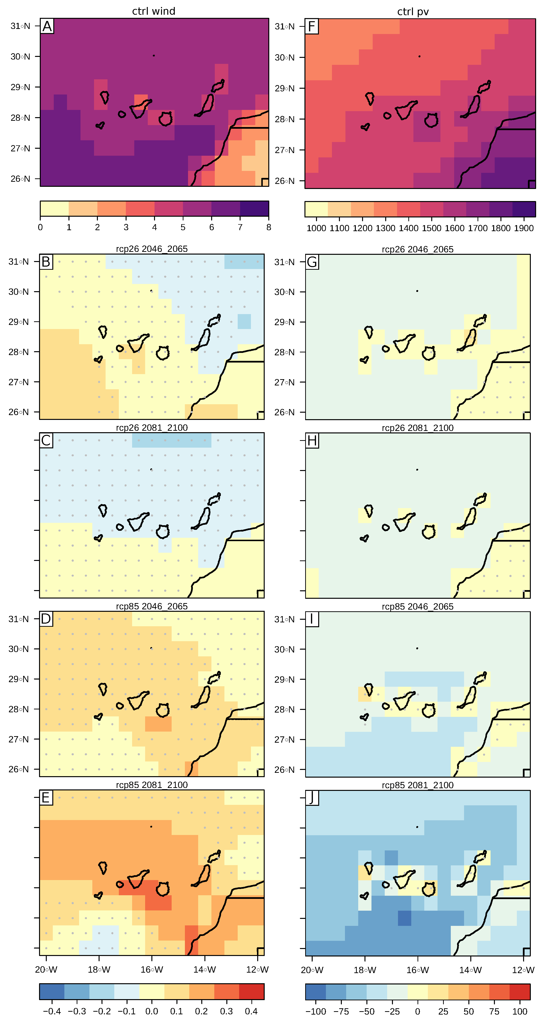
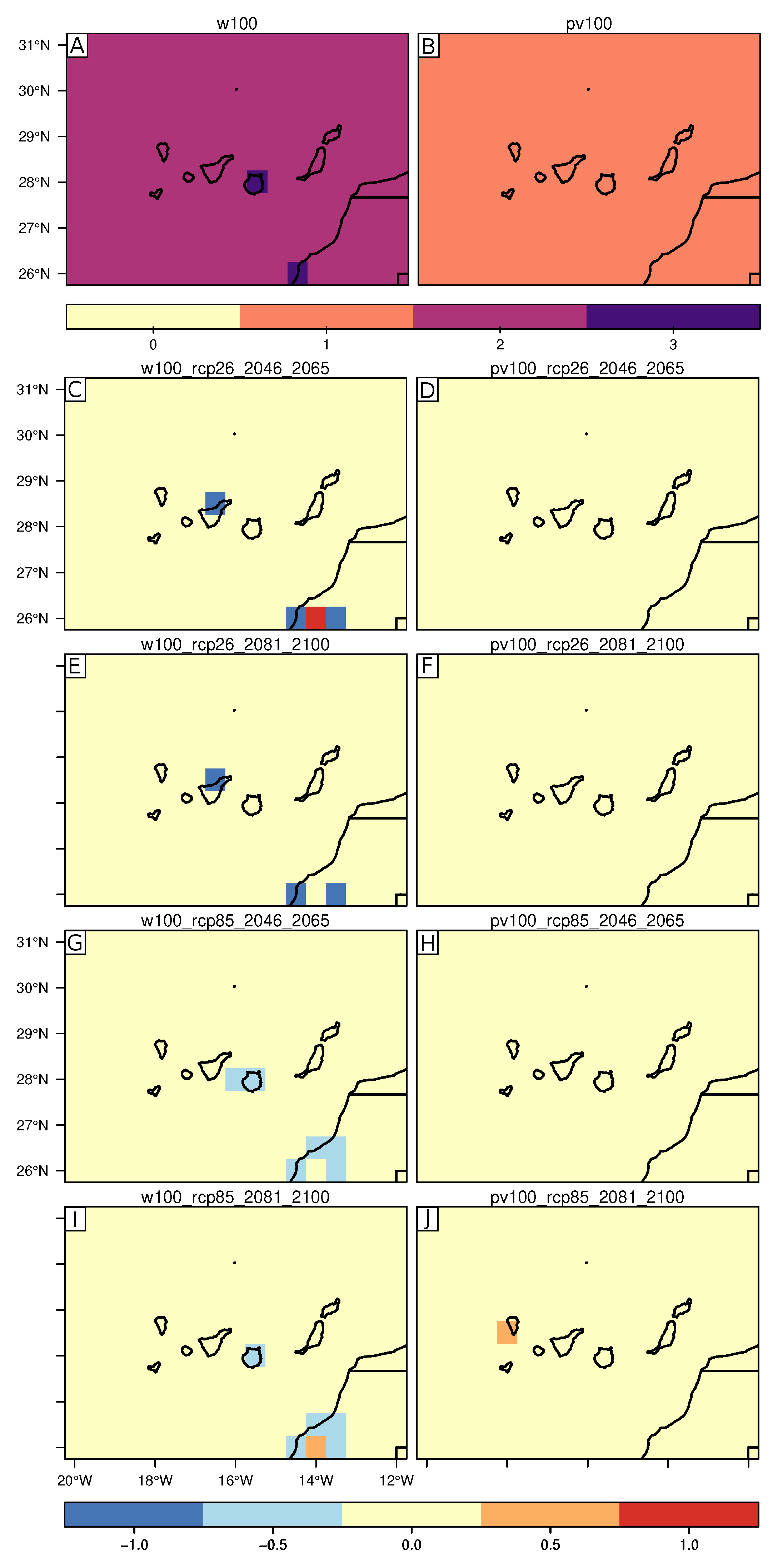
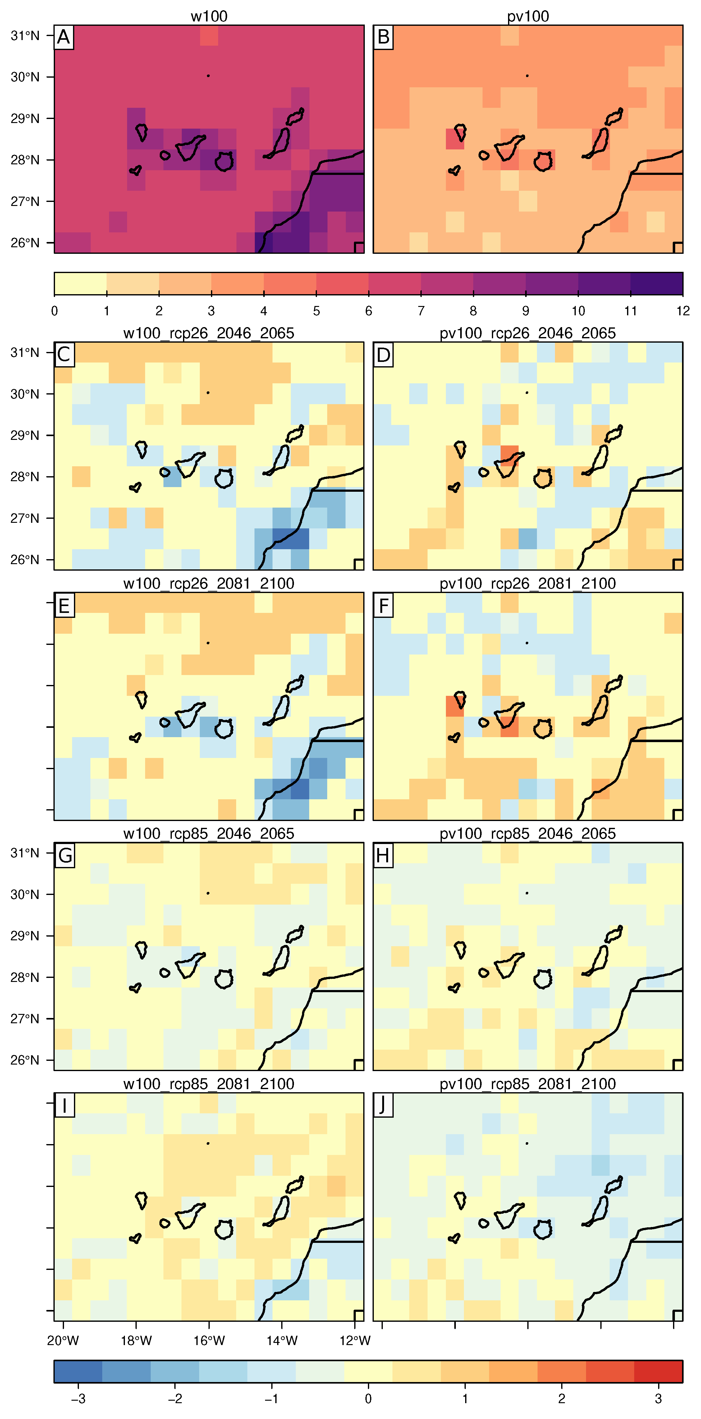
In the control time period, wind and PV productivity showed important differences in terms of magnitude and regional distribution. Starting from wind productivity we observed that it is greater over the sea than over land (
Figure 1A). This is related to the lack of obstacles over the marine domains and the higher hub height in offshore wind turbines. Within the islands, wind productivity is close to 2000 kWh/kW, whereas it takes values of about 5000–6000 kWh/kW over the oceanic areas adjacent to the archipelago. PV productivity shows the largest values over the African continent, reaching a locally-maximum value close to 1800 kWh/kW (
Figure 1G). Over the sea, smaller values of PV productivity towards the NW can be observed, with the minimum values reached close to 1400 kWh/kW.
As to future changes in wind productivity, we observed that the spatial pattern is set by the chosen time period (
Figure 1B–E). In the RCP2.6 scenario, a subtle increase to the SW of the considered domain can be observed in the 2046–2065 period, but a general decrease in the northern half of the domain is projected by the end of the century. In the RCP8.5 scenario, a productivity increase which is even more pronounced by the end of the century, with a maximum increase close to 300 kWh/kW near Tenerife, Gran Canaria and the African coast, is projected. However, most of the changes are not singnificant, in most of the domain, with the exception of the RCP8.5 by the end of the century. This result of the increase by the end of the century and at the mentioned areas is consistent with results presented in [
14,
15], in which the authors found a generalised intensification of the North African Coastal Low-Level Jet. That means more frequent and intense winds at the north western African coast, which is likely to occur for every season. In the case of PV, all scenarios and time periods show an overall, but subtle, decrease in productivity for the studied domain in marine areas, of higher magnitude for the RCP8.5 scenario and statistically significant in most cases. Smaller changes are found over the islands in agreement with [
13], where non-significant changes are projected in annual terms.
3.2. Changes in Variability: Wind and Photovoltaic Droughts
In order to study the variability of wind and PV resources separately, we focused on the study of the frequency of droughts (expressed in % of drought days within the considered time period), as well as the number of consecutive drought days (cdd, expressed in absolute terms, days). We calculated all the events with more than one consecutive day of drought and we analyze the longest event. This provides an estimation of the propensity of the generation to drop below a critical level and the persistence of those events. In addition, the longest consecutive drought days event was important in order to estimate how long could the PV and wind production persist below the normal to plan storage or backup facilities.
3.2.1. Frequency of Wind and PV Droughts
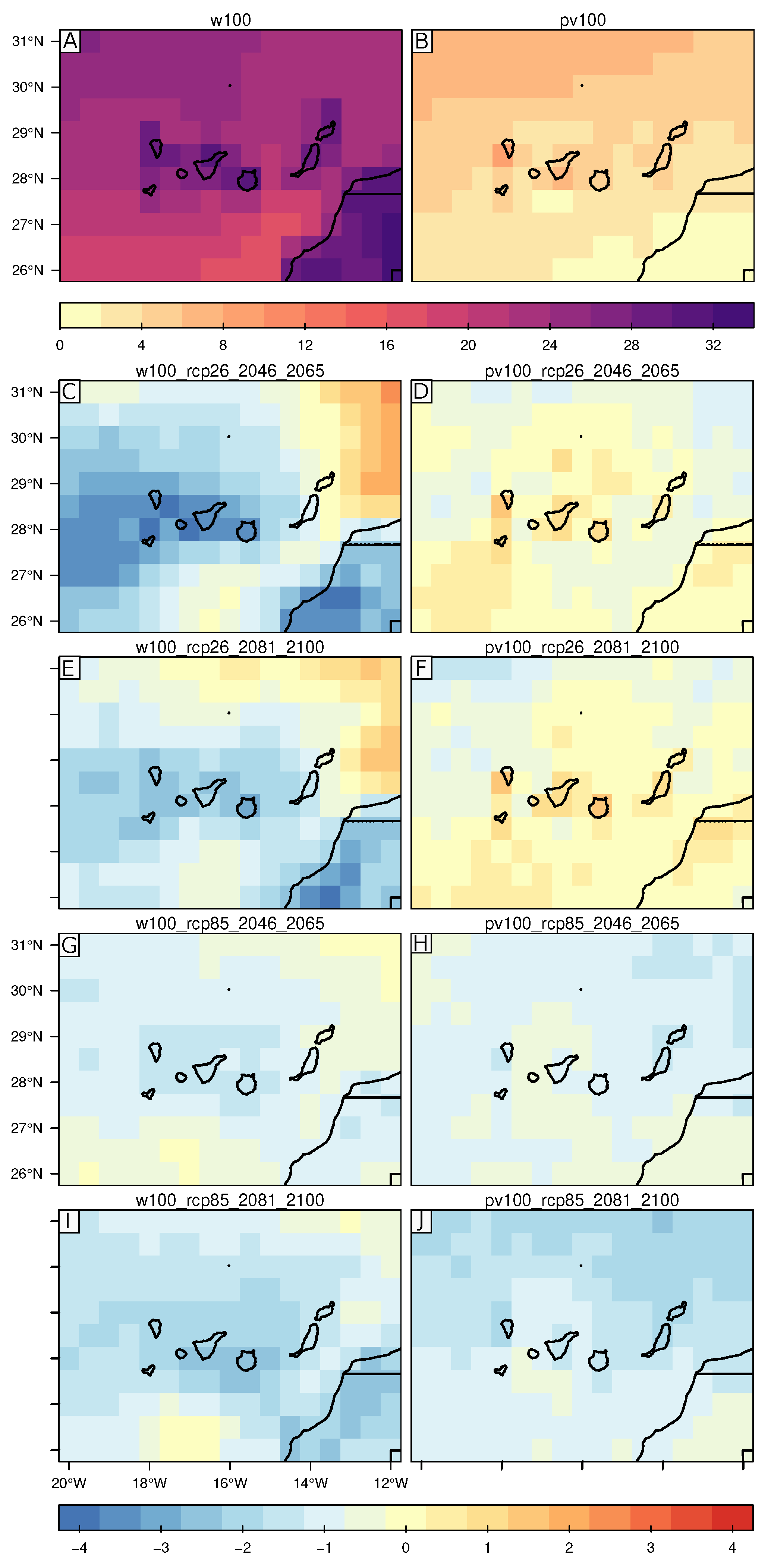
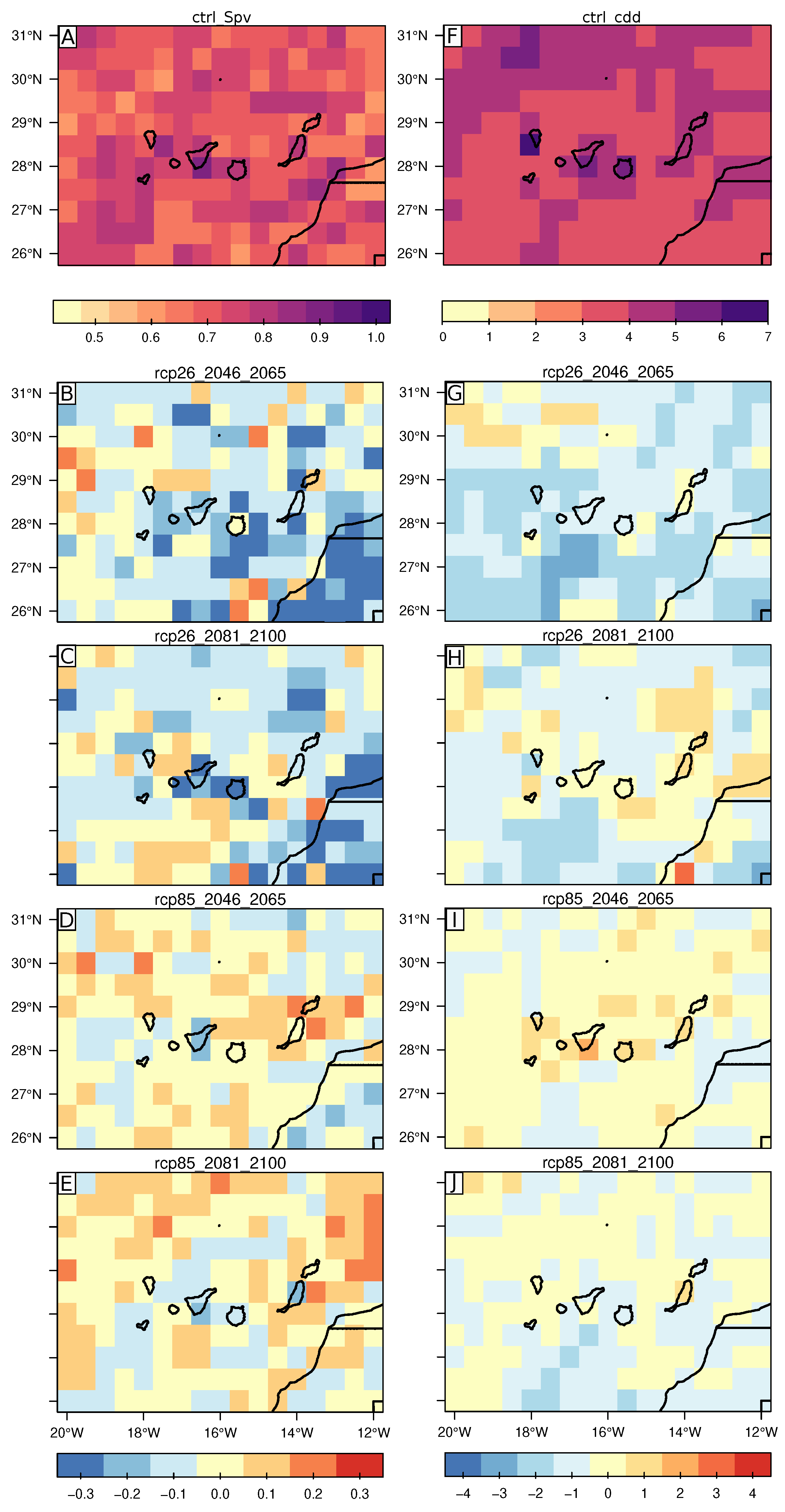
As an estimation of wind and photovoltaic variability, the study of the frequency of droughts from each source i.e., 100% of the energy derived from that source (
Figure 2), is made. In the control time period, wind droughts were more frequent over land than over the sea (
Figure 2A), whilst over land, they took values close to 30%, the corresponding percentage of drought days is smaller over the sea, with values ranging from around 15 to 25%. This may be driven by the lack of obstacles in marine areas which reduce productivity variations over time. On the contrary, when all the energy comes from PV generation, the frequency of droughts becomes substantially smaller (
Figure 2B). In this case, the percentage of droughts did not exceed about 5% of the days. Whilst PV productivity was smaller than wind productivity, it was less variable and thus ensured a smaller number of days with drought conditions and a more sustained production over time. Comparing this results to previous analysis over different regions, we observed that the percentage of drought days over the Canary region was in general lower than for the Mediterranean Islands [
29].
Regarding future energy droughts for wind and solar productivity, respectively (i.e., RCP2.6, RCP8.5;
Figure 2C–I), wind droughts feature a slight decrease in the percentage of drought days over most of the domain regardless of the scenario and time period considered. The greatest decrease appeared in the near future (2046–2065), in the RCP2.6 scenario. In this case, a decrease was projected over most of the considered domain, with the exception of the north–eastern side of the domain. A similar pattern was observed for this scenario by the end of the 21st century, but with smaller differences with the control period.
Interestingly, solar productivity droughts present a clear pattern which depends on the emission scenario chosen (
Figure 2D–J). On the one hand, a slight increase in the percentage of drought days is generally projected over under the RCP2.6 scenario. On the other hand, a decrease in the percentage of drought days compared to the control period occurs in all the studied periods under the RCP8.5 scenario. Moreover, under this scenario, a marked latitude-dependent pattern can be observed in the 2081–2100 period, with a larger decrease in the frequency of PV droughts to the north of the domain. Results presented so far highlight that, whilst changes in the frequency of PV and wind droughts, respectively, are relatively small (i.e., not larger than five percentage points in magnitude), different patterns can be found depending on the energy source, time period and scenario considered.
3.2.2. Consecutive Energy Drought Days
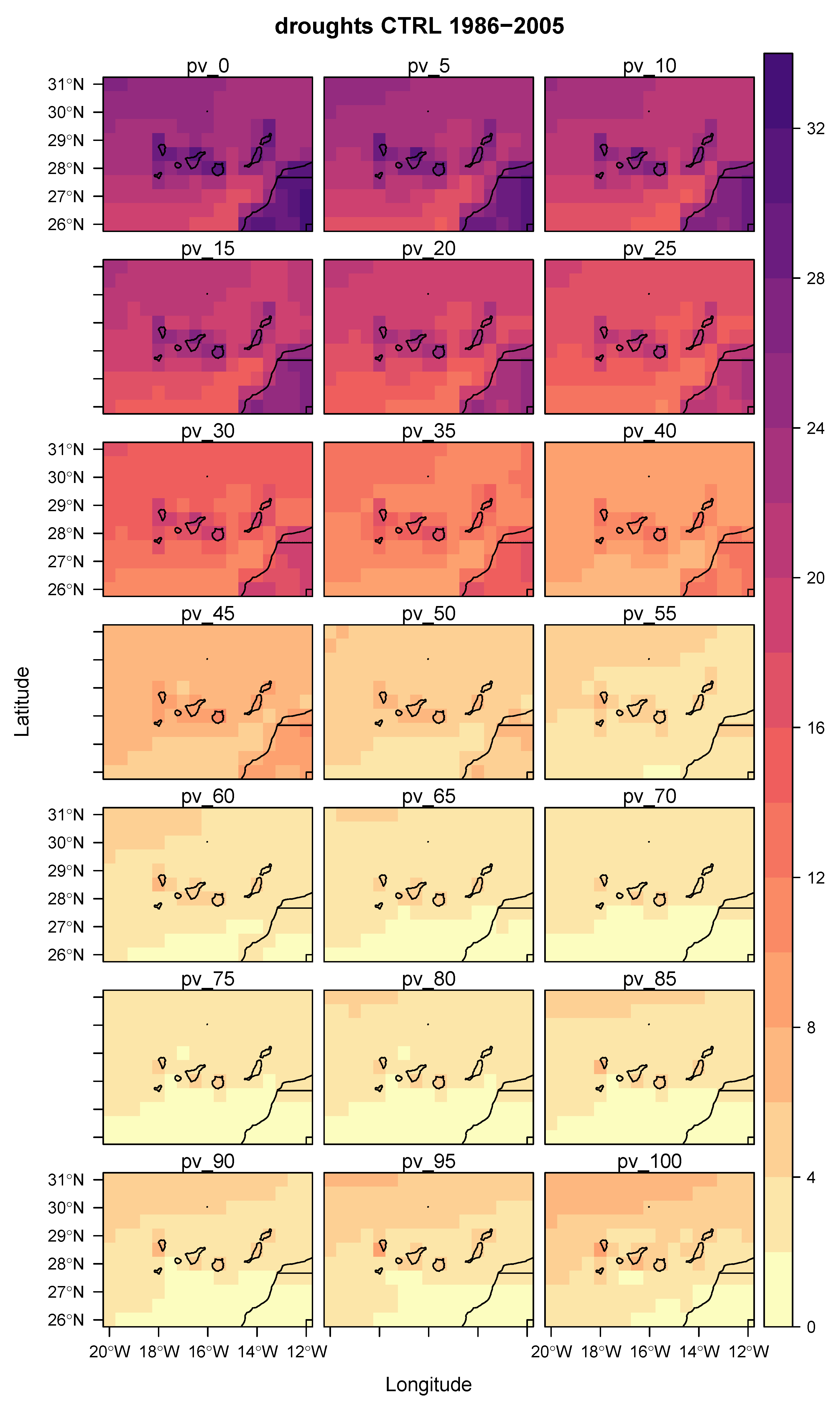
Drought days have been defined as those in which energy production is below a given threshold (see methodology in
Section 2). That situation can persist up to several days, becoming an event of consecutive drought days. Drought events usually last 2 to 3 days in the control period, for wind and 1 day for PV technology (see
Figure A1 of the
Appendix A). However, longer periods of drought conditions are also possible and can affect stability of the supply as well as the planning of the energy system, due to the higher amount of needed storage. Due to that, the longest events for each source in the control period, as well as their future changes, are evaluated in this section.
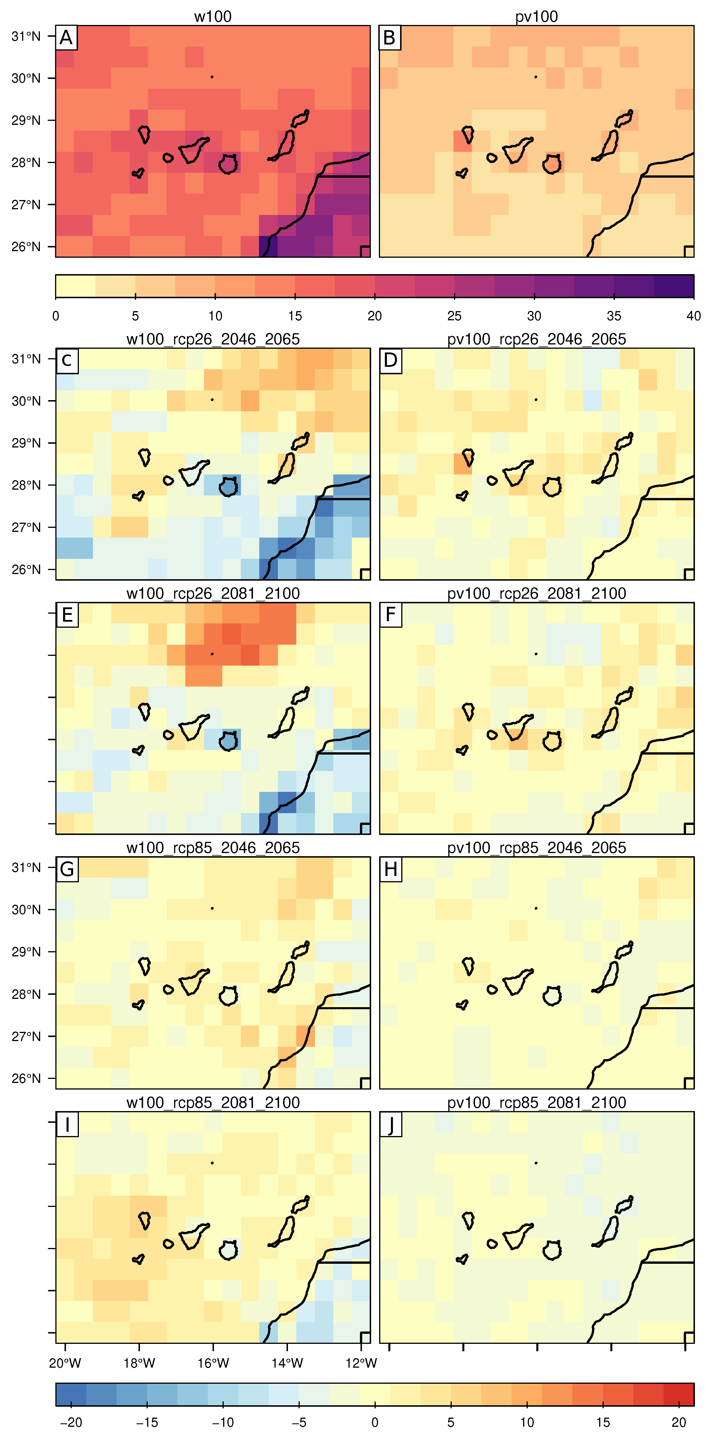
In the control time period, in line with what has been found in the frequency section, wind productivity is more prone to experience longer periods of drought conditions compared to PV productivity (
Figure 3). In land areas along the African coast, the longest event for consecutive wind productivity droughts was close to 40 days, whereas in the case of PV, the longest event lasts around 10 days over the islands. Values of the 95 percentile of cdd for both resources can also be seen in
Figure A2, where the same pattern is observed, but with smaller values. For wind, the 95 percentile was around 11 days and 4 in the case of PV cdd.
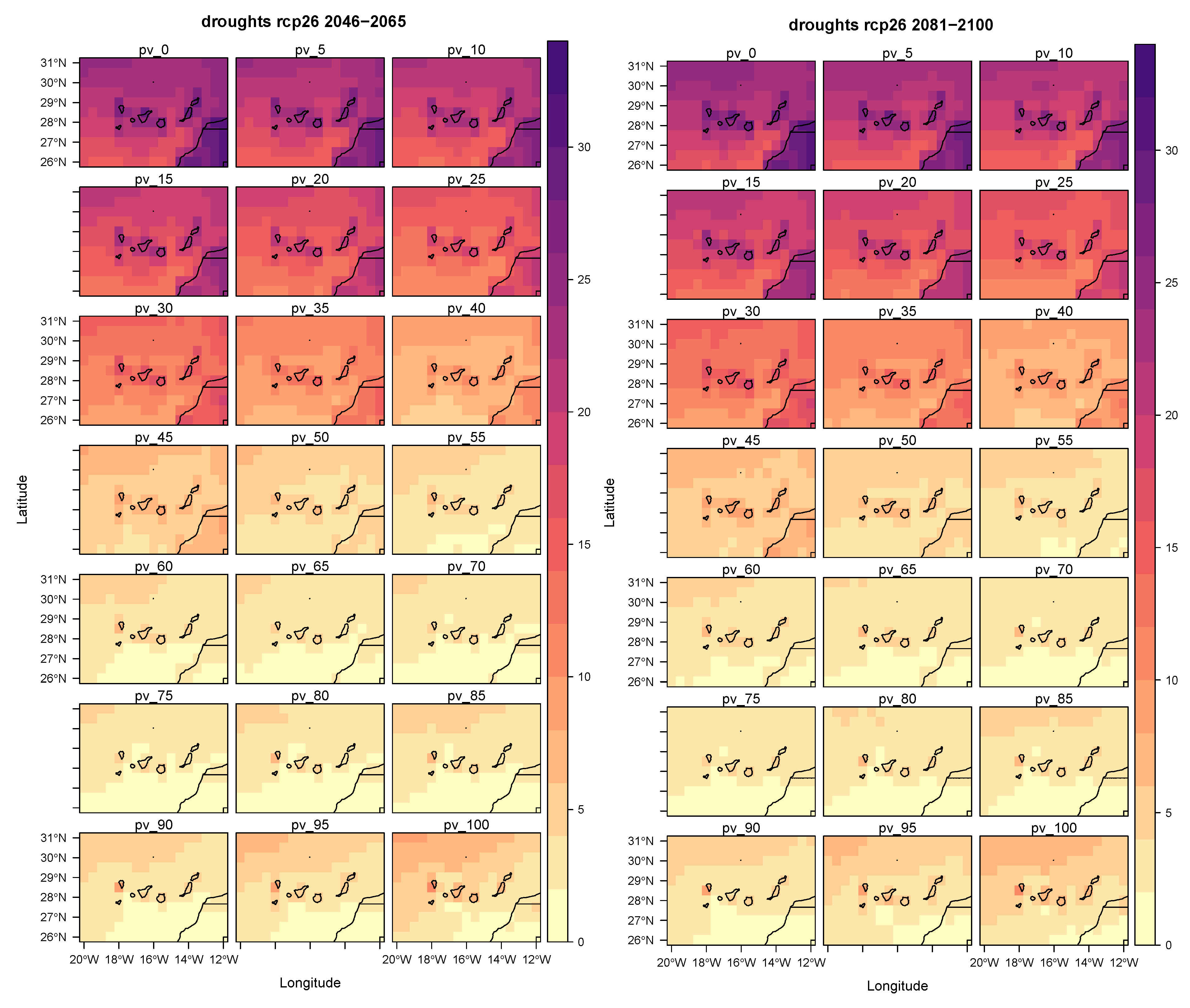
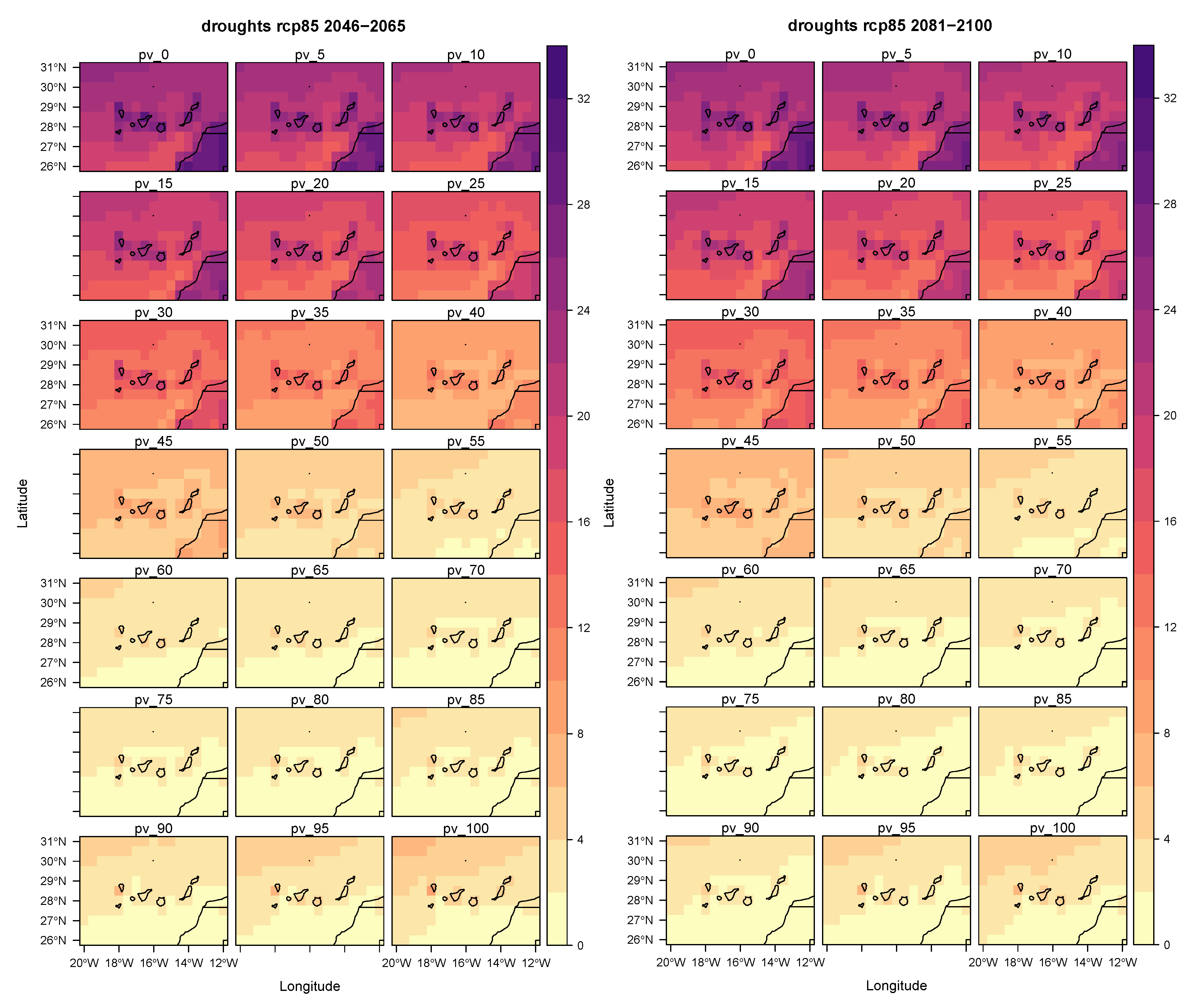
Regarding future changes in the cdd, although there were almost no changes in the median value of the length of cdds (
Figure A1), meaning that in the future most of the drought events will continue to last 1 to 3 days, some changes were found in the extreme values. We observe that different patterns can be distinguished for the wind and PV cases (
Figure 3C,D). In particular, regardless of the time period and scenario chosen, the maximum of wind cdd decreases over the African continent, with a maximum decrease up to 15–20 days for the longest event. Elsewhere, the number of cdd shows a generalised, but subtle, increase with the exception of RCP2.6 by the end of the century, when a remarkable increase close to 15 days is projected north of the Canary Islands. Moving to the cdd concerning PV productivity, differences are, in general, of a smaller magnitude than those encountered for the wind. Specifically, in the RCP2.6 scenario, an overall increase of cdd up to a maximum value of about 5 days occurred over most of the domain in the two time periods considered. In the RCP8.5 case, changes were even more subtle than in the RCP2.6 scenario. In
Figure A2 changes of the 95 percentile present great spatial variability for both resources, but with small changes as in the longest event projections.
3.3. Changes in Complementarity
After the analysis of variability changes for each source, an assessment of how the different combinations of PV and wind energy could affect the energy output intermittency (i.e., the frequency of drought days and the number of cdd), is presented in this section. A sensitivity test that varies the share of PV energy (Spv) from 0 to 1 (and in each case the corresponding wind energy Sw = 1 − Spv) with an increment of 0.05 in each step was made to obtain how complementarity between both resources changes. Values of Spv multiplied by 100 were the equivalent percentage of PV technology considered. In some of the sensitivity simulations performed, the amount of Spv that leads to minimum was not a unique value, which means that different shares of PV would result in the same percentage of drought days. Here, we have considered the combination with the lowest amount of Spv. Other restrictions could be applied in different studies.
3.3.1. Frequency of Drought Days
Values of PV and Wind to Minimize the Frequency of Drought Days
The optimal combination of PV and wind (values of Spv and Sw), to reduce the frequency of drought days to a minimum is obtained from a sensitivity test (explained in the methodology section) that analyzes different percentages of PV and wind production in a scenario that considers only these two sources.
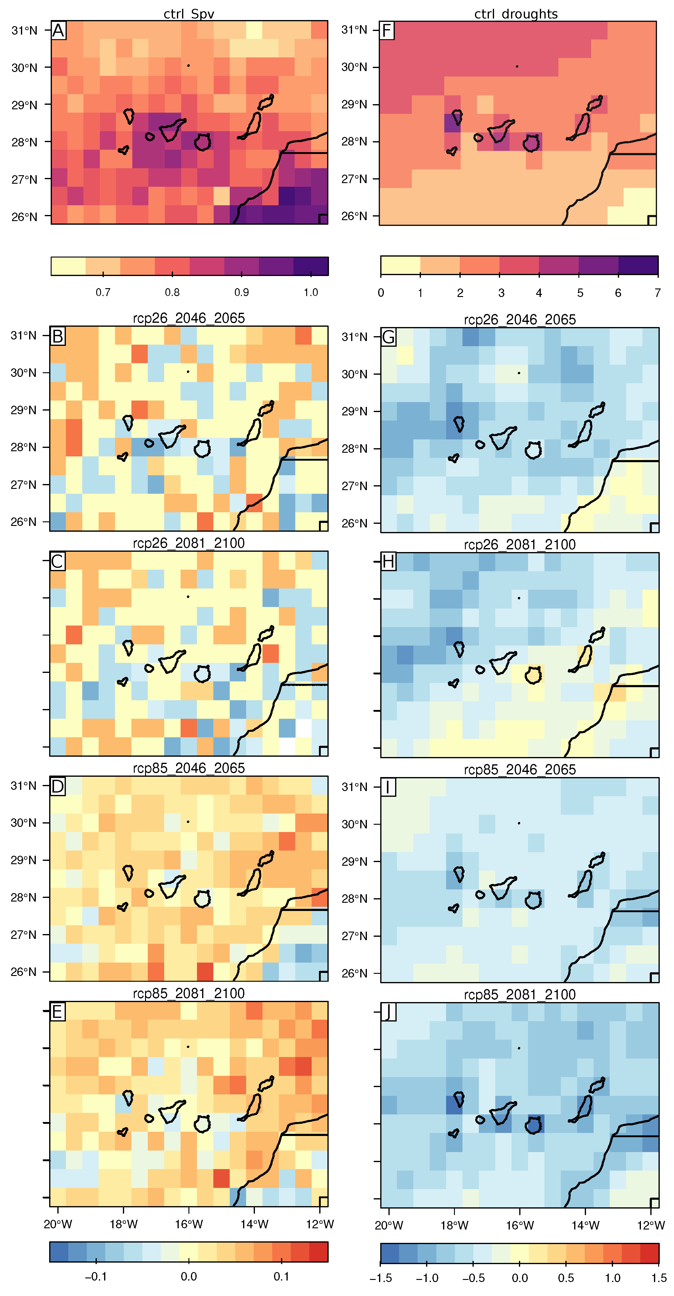
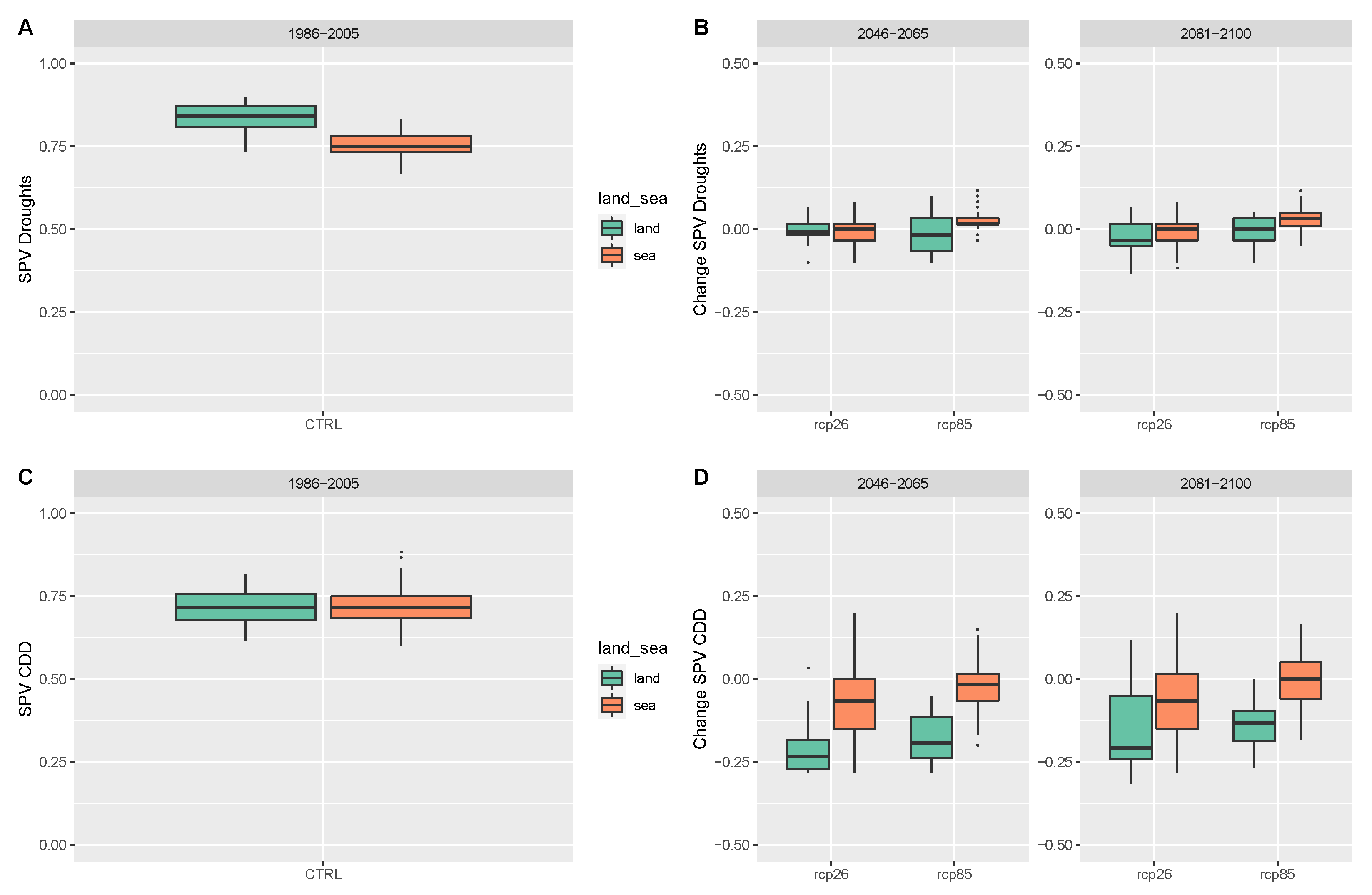
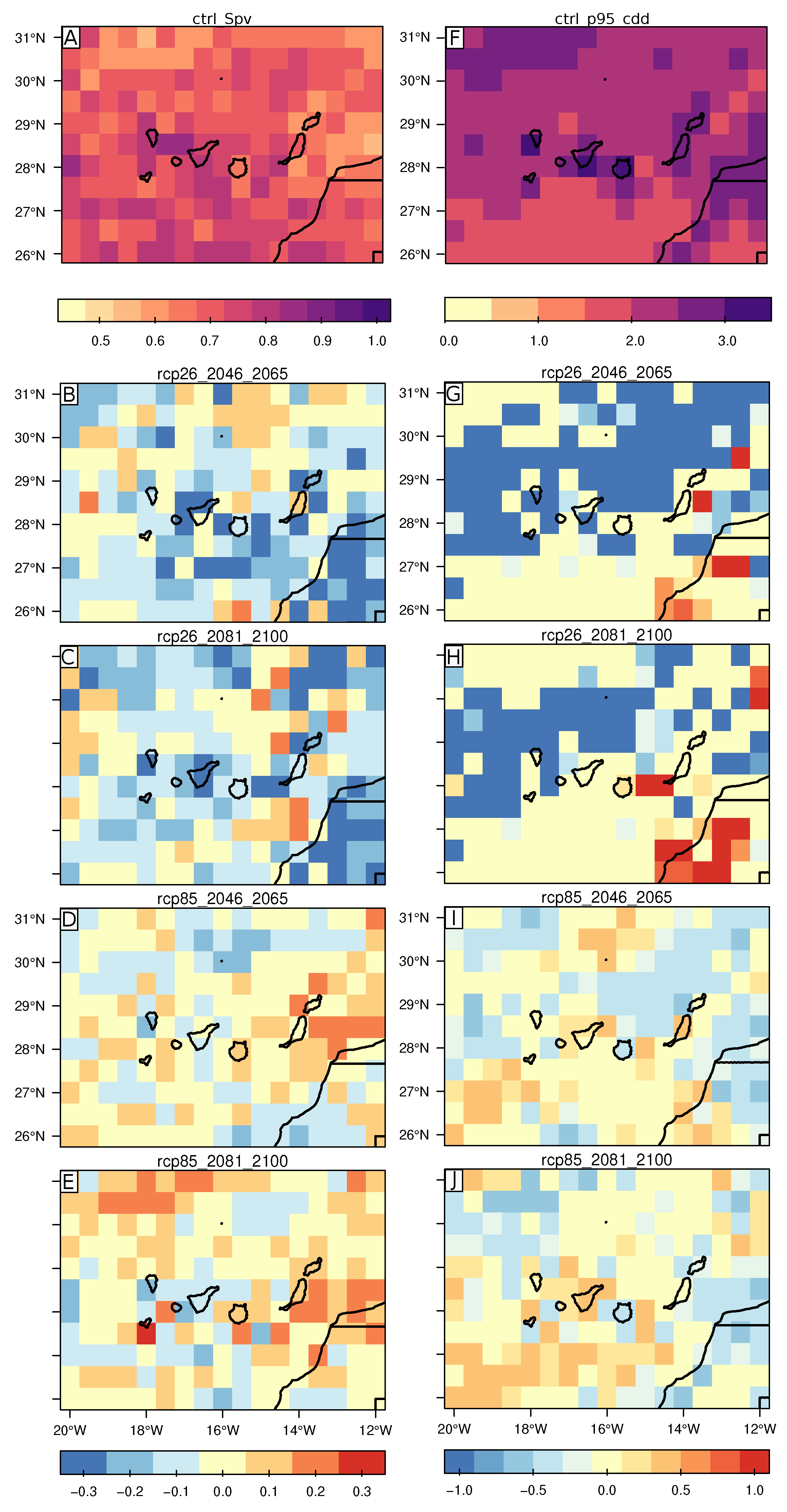
Figure 4 shows the values of Spv i.e., the percentage of PV energy which leads to the optimal combination for each cell in the control time period, as well as future changes with respect to the control. In spite of the great spatial variability, optimum values of PV are always greater than 65% (Spv of 0.65) either in the control period or in the scenarios (
Figure 5A,B). This indicates that an important share of PV energy is necessary to decrease the frequency of drought days to its minimum. A compilation of the battery of results obtained with different combinations of PV and wind for the control time period can be found in
Figure A3 of the
Appendix A. A clear decrease in the frequency of droughts is seen when the amount of PV energy increases. Changes in the frequency of drought days are subtle when more than 50% of PV is considered.
In the control, interestingly, the optimum Spv was higher over the African continent, with values as high as 0.80–0.95 (
Figure 4A) and lower values of Spv are found in the north of the domain (0.65–0.70), where wind productivity is larger. This was the result of two factors: first, wind variability is larger over land than over the sea, which is consistent with the fact that marine wind productivity is higher due to the lack of obstacles. Second, PV variability was also lower in the southern part of the domain and over African continent (
Figure 2B). This pattern is observed in
Figure 5A, with, in general, lower Spv values over the sea, with a median value of 0.75 (75% of PV share) compared to the median value over the land, which is around 0.85 (85% of PV share).
Differences in the optimum PV values for the RCP2.6 and RCP8.5 scenarios with respect to the control period show great spatial variability over land and over the sea (
Figure 4B–E). We note that the optimum values of Spv are in some locations, in the RCP2.6 scenario, lower than in the present case, although the presence of a spatial pattern is not straightforward (
Figure 4B,C). This indicates that combined variability does not show a clear pattern with a spatially-dependent increase or decrease of steadiness with time. However the fact that Spv becomes smaller in some areas is consistent with a decrease in wind variability in the future combined with an increase in PV variability as seen in
Figure 2. When differences between land and sea cells are considered (
Figure 5B), small differences (non-significant) are found in the median values for Spv with respect to the control in both periods either for land or sea cells.
Regarding the RCP8.5 scenario, we note that, with the exception of some islands and a great part of the continent, there is a prevailing increase in Spv with respect to the control in certain areas. As for the RCP2.6 scenario, there is large spatial variability in this case. Values of Spv appear to be larger than at present over the sea in both periods (75% median value of PV share in control period and close to 80% in future periods) and small changes are found over the land (
Figure 5B). It is important to note that, in some of the sensitivity simulations performed, the amount of Spv that leads to minimum energy droughts is not a unique value, which means that different shares of PV would result in the same percentage of drought days (
Figure A3,
Figure A4 and
Figure A5).
Minimum Number of Drought Days Using the Optimal Combination of PV and Wind
We now examine the frequency of drought days in the control time period when the optimal combination of energy is considered, as well as future changes relative to the control (see
Section 2 for details of the methodology),
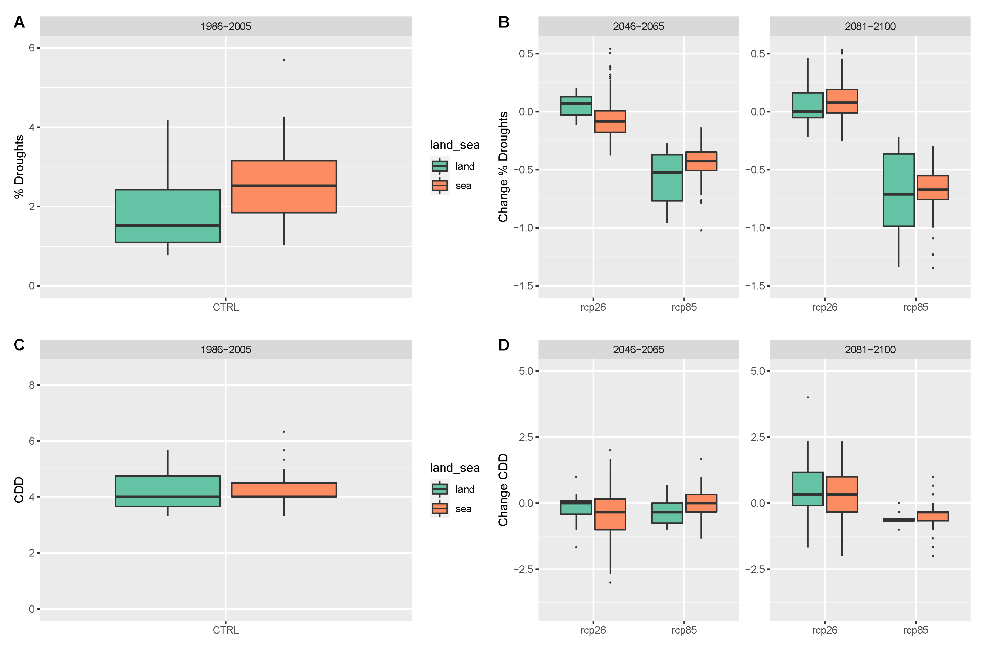
Figure 4. We note that, in the control time period, the frequency of drought days does not exceed about 7% of the days (
Figure 4F), which is remarkably lower than the percentage obtained for wind productivity alone. A marked NW—SE gradient exists, with the highest values to the NW. This gradient seems to be triggered by both wind and PV energy, which present a qualitatively similar regional distribution in terms of frequency of energy droughts. However, differences of magnitude between them are observed. In addition to this, local maxima of the drought frequency for wind can be found over the islands. This can also be observed for the wind-PV combination. This may be caused by the fact that wind productivity is smaller and more variable over land due to the presence of obstacles. However, when the frequency of drought is aggregated by land or sea cells, respectively, it is observed that there are lower values of droughts over the land, with median value around 1.5% compared to median sea value, 2.5% (
Figure 6A). This is due to the minimum observed over the African continent, that minimizes the impact of the Canary Islands values.
Regarding future changes in the minimum frequency of drought days, in general, these present a decrease in the RCP2.6 scenario but with subtle positive changes in some islands, the African coast and the south of the domain by end of the century
Figure 4G,H. Whilst a generalised decrease in the occurrence of drought days occurred under the RCP8.5 scenario with a more prominent lowering in the 2081–2100 period (
Figure 4I,J). These changes can be observed grouped by land and sea cells in
Figure 6B. In particular, the RCP2.6 case presents non-significant changes and only in the 2046–2065 positive increase in median value can be observed by the end of the century for sea cells, whereas land cells present similar values, with some local increases. As to changes in the frequency of droughts in the RCP8.5 scenario, we observe a generalised decrease (statistically significant) in the percentage of drought days regardless of the time period considered (
Figure 4I,J). The reduction is especially important by the end of the 21st century, particularly over the CI, which can be seen in
Figure 6B. By the end of the century median value of droughts for land cells decrease around 0.75. This is in agreement with the decrease in drought days observed in the scenario of 100% PV and 100% wind productivity projections respectively.
3.3.2. Maximum Number of Consecutive Drought Days
Values of PV Energy to Minimize the Maximum Number of Consecutive Drought Days
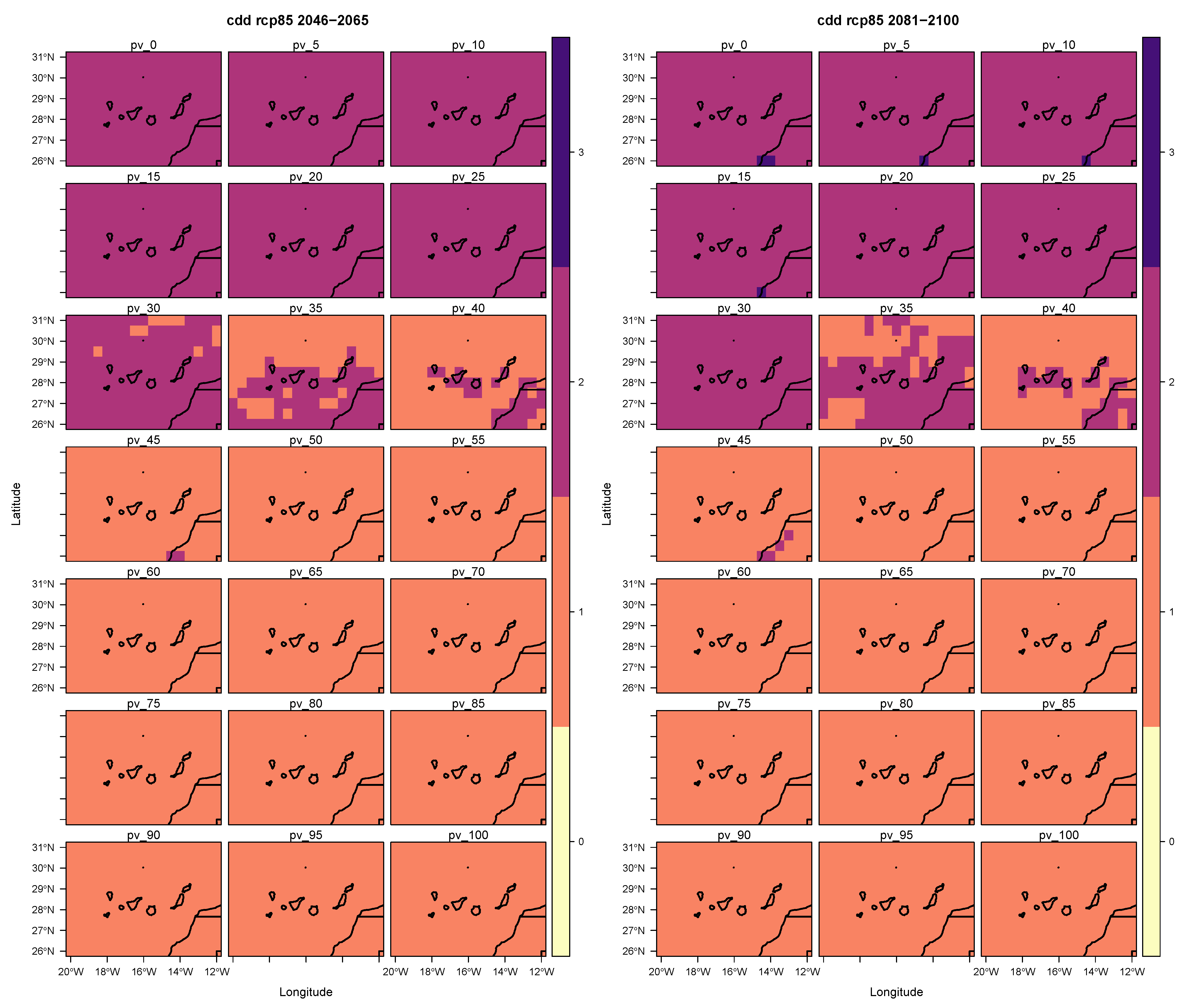
As for the frequency of drought days in the previous section, the optimization assessment is made in order to obtain the PV share (Spv) that minimizes the length of the consecutive drought days events, cdd. Usually, drought events last from 1 to 3 days (median value) in the control period and very similar results are obtained for future periods, regardless of the scenario (see
Figure A1) and the amount of Spv (
Figure A9,
Figure A10 and
Figure A11). Therefore, there are different values of PV share that would minimize the length of these events to 1 day and it is also possible to find this minimum in the scenarios (see
Figure A1).
However, although events of 1 to 3 days were the most common ones, longer periods of drought conditions can impact the stability of the supply and it is thus important to detect the optimal combination of resources that minimize extreme events in the control period as well as their future changes. In the control time period (
Figure 7A), values of Spv are always greater than 0.6 (60%), with a median value around 0.7 (70% of PV share) for both land and sea cells (
Figure 5C), which means that PV energy has to prevail over wind energy in order to minimize the length of the maximum cdd event as seen for the minimization of the frequency of drought days. No clear spatial pattern arises in the control period. Maximum values of Spv close to 0.9 can be found to locally minimize the longest cdd event. As to future changes (
Figure 7B–E), we can see that these also present large spatial variability. There is a maximum in the magnitude of the absolute changes close to 0.3 positive (increase in the Spv share) and negative (decrease in the Spv share). Minimum value changes are found for the RCP2.6 scenario, which shows overall changes of greater magnitude regardless of the time period compared to RCP8.5 (
Figure 7B–E). In spite of the large spatial variability and local maximum, changes in the RCP2.6 scenario (
Figure 7B,C) tend to be negative as seen in
Figure 5D (a decrease in Spv leads to a minimization of the length of cdd). A clear decrease in Spv is seen over land for RCP2.6 in both periods. For the RCP8.5 case, there is large spatial variability and some islands show a clear decrease in the optimum Spv, like Tenerife (
Figure 7D,E). We observe an increase over the sea, higher at the end of the century, but a decrease over land in both time periods (
Figure 5D), more important for 2046–2065.
Maximum Number of cdd Using the Optimal Combination of PV and Wind
As seen in the previous section, there was a wide range of values that minimize the most common length of cdd to just 1 and this also happens in future periods regardless of the scenario (see
Figure A1). Although there was no change for the median length of consecutive drought days, cdd, we note differences in the extreme cases of cdd. In
Figure 7F–J we observed the maximum number of cdd of the considered time period making use of the optimal percentage of each technology for the control, as well as the corresponding future changes. We note that, in the control period (
Figure 7F), the longest event of cdd never exceeded about 7 days and the median value is around 4 over the sea and over the land (
Figure 6C). The number of maximum cdd was higher in the islands than in the marine areas adjacent to them. A maximum was found over La Palma island and a north-to-south gradient with larger values to the north of the domain can also be distinguished. On the contrary, the 95 percentile of the cdd was reduced to a maximum of three consecutive days when the optimal Spv was considered, as we can see in the
Appendix A (
Figure A12).
Regarding future changes in the longest cdd event relative to the control we observed that differences were small with a local maximum of 3 days for changes in RCP2.6 by the end of the century (
Figure 7H). The spatial pattern shows a more generalized decrease for RCP2.6 (with some regional exceptions at the ned of the century) and more subtle changes in RCP8.5. In addition in all the different time periods and scenarios tested (
Figure 7G–J), the southern portion of the domains tended to experience a decrease in the maximum cdd event. For the RCP2.6 scenario, the median value of the maximum cdd was around 4 in the 2046–2065 period and increased to 5 at the end of the century over the land, whereas sea changes were smaller. Changes founded for the RCP8.5 scenario grouped by land or sea cells were small, with a subtle decrease more noticeable (and significant) at the end of the century either for land and sea (
Figure 6D).
3.4. Implications
The availability of renewable energy resources could change in the future because of the impact of climate change and the possibility of evolving through different emission scenarios, as we have seen in previous sections. For that reason, the study of the future evolution of these resources is specially important to reduce greenhouse gasses emissions (GHG) derived from energy generation and provide the necessary tools to accelerate the sustainable energy transition. In regions of insular nature, which are highly dependent on energy imports, this assessment could help in the planning of a system with some particular characteristics, like the land–surface limitations for the deployment of large generation plants. Due to that, the assessment of offshore resources becomes more important in these areas. Wind and photovoltaic (PV) technologies, which will be likely the most important renewable technologies for the new generation system, present high potential in the Canary Islands and their adjacent marine regions. Our results indicate that in the future, wind resource may slightly decrease or increase, depending on the future emissions evolution In the case of photovoltaic resource, it will change only slightly regardless of the scenario, in good agreement with a previous study with a single model [
13].
In general, uncertainty related to climate models, has been seen as a constraint for the applicability of climate models in policy. In spite of that, different research works encourage policymakers to include climate models projections in their decision tools. In the present work, the uncertainty in the climate change signal of the wind resource could be seen as a limitation in order to advise policymakers in terms of investment. However, the fact that greatest disagreement among scenarios happens at the end of the century, facilitates the use of climate model results because planning strategies on immediate infrastructure can be made with near-future projections, that present small differences between scenarios.
As the intermittency of renewable energy has been one of the main constraints during their integration into the grid, it is worth evaluating whether the variability of these resources could change in future climate. The concept of energy drought is used to indicate the frequency of days in which renewable energy production is below a given threshold and to estimate the maximum number of consecutive drought days. In present climate, wind productivity presents a much higher frequency of drought days compared to photovoltaic productivity, which shows a more steady pattern. In terms of future climate, small changes are seen in the variability of both technologies, which is and advantage in terms of planning backup infrastructure. As a strategy to overcome the limitation due to daily variations in renewable energy generation, the complementarity between different technologies becomes a possible solution. When a combination of PV and wind energy is considered at each location of the domain, a reduction in the output variability is found in terms of a decrease in the frequency of drought days and the length of drought periods.
We look for optimal combinations with the objective of reducing variability, and it is found that PV share should be higher than wind share. PV share should be about four times higher than wind over land, and about three times higher over the sea in order to optimally reduce the frequency of drought days. The optimal PV capacity share is, in general, lower in marine regions, where the wind productivity is more steady. When the objective is to reduce the longest event of consecutive drought days, the optimal PV share is lower, but in any case larger than the wind share. These results can be compared to other studies made in different regions, which have shown that the optimum values of PV for reducing variability in areas with high solar resource are above 50% [
44,
45]. Certain studies give different results depending on the time frequency analysed [
43]. In any case, the fact that a combination of resources reduce most of the times the variability of the energy output is clear.
There is a strong need for including complementarity between different renewable technologies in energy planning schemes [
46], as an adequate application of this characteristic can reduce the reserve requirements and the uncertainty in generation costs. A deployment process centered on installing the least costly energy source at the most productive sites can end in a highly unbalanced generation mix. To avoid such outcomes, complementarity criteria should also be included in renewable energy support mechanisms. There is a debate between the convenience of using technology-neutral or technology-specific approaches [
47], as technology-specific policies allow to incorporate criteria beyond electricity prices and can be cost-effective in the presence of market failures and social costs. Many renewable energy auctions have focused on promoting the least costly installations, but auction designs can incorporate complementarity criteria or even enforce wind-solar hybrid installations [
48].
The results obtained here present the limitation that the space needed for PV plants with the same capacity than a wind farm is larger, which in some cases could be a problem for island regions. However a more detailed analysis including other factors in the optimization process (like economic factors as prices and cost) is beyond the scope of this paper, and could be considered in a future research. In addition, the objective function could be adapted depending on the strategy to be followed, for instance reducing seasonal variability instead of daily variability. Further research should include a more comprehensive approach for system modeling, considering other generation sources, but in any case climate information should be used in the assessment of the resources.
4. Conclusions
An evaluation of the resources and their future variability is of special interest for the different stakeholders to efficiently manage planning of new power infrastructure. For that reason, the use of climate simulations to evaluate climate evolution in different possible scenarios is a necessary tool.
In this work, we have seen that in the RCP2.6 scenario, regardless of the time period examined, wind productivity experiences a more generalised decrease by the end of the century. However, in the RCP8.5 scenario, a remarkable increase in wind productivity is projected, especially by the end of the century. As to PV changes, all scenarios show an overall decrease of productivity in the studied domain with changes of a small magnitude, with the exception of the islands, where changes are subtle or slightly positive.
The variability of wind and PV resources can be described by the frequency of energy drought days, which we define as the frequency of days (in %) that the productivity of each resource is under a given threshold. Wind droughts are more frequent than PV droughts and, in general, an event of several consecutive drought days (cdd) has a duration between 1 and 3 days. However, the longest event can reach about 40 days in the case of wind energy and only more than five days in some areas for PV. In the future, wind droughts feature a slight decrease in the frequency of drought days over most of the domain regardless of the scenario and time period considered. Interestingly, PV productivity droughts present a clear spatial pattern which depends on the emission scenario chosen. A small increase in the percentage of drought days is generally projected under the RCP2.6 scenario, whilst a decrease occurs under RCP8.5.
In terms of the persistence of drought conditions i.e., cdd, future projections show a general, increase of the longest event for wind energy regardless of the time period and scenario, with an important decrease along the African coast and some islands. The reduction of the length in the maximum cdd is bigger for RCP2.6, coinciding at the same time with some areas where wind productivity decrease is projected. Small changes are found for PV energy, although these are positive in general with the exception of the RCP8.5 scenario by the end of the century. These results highlight that the strategy adopted to address the lack of production for several cdd, hardly needs to change in the future.
The optimal combination of PV and wind energy required to reduce droughts of combined energy production have, in general, PV shares greater than 65% regardless of the scenario or time period chosen, as well as a median value of around 70% over the sea and around 85% over the land, which highlights the greater stability of PV energy over time with respect to wind energy. The frequency of energy droughts when the optimal combination is considered, which is larger over the sea (1.5%) than over land (2.5%) although small in both cases, is generally reduced for both scenarios, but an increase over land is found in RCP2.6 by the end of the century. At that time, the projected frequency of drought days in the RCP8.5 scenario is 1% over the land and 1.5% over the sea. In summary, the optimal combination of wind and PV energy in each period, mostly conformed by a high share of PV, would benefit the total energy production reducing the variability, i.e., frequency of drought days to a very low value. However, the amount of PV energy necessary to reduce this varibility to a minimum would require a great occupation of space, due to the technology characteristics. For that reason, the necessary constrains in each case should be considered specifically.
In order to reduce the length of the longest drought event, changes in the optimal combination of PV and wind show great spatial variability and, in general, the longest event is either reduced or increased in 1 day in general, regardless of the scenario or period. Values of PV share to minimize the longest event of cdd are generally lower than for minimizing the frequency of droughts, but always above 50%. Opposite to the Spv for minimizing drought days, Spv tends to be larger over sea cells, than over land. The optimal combination of PV and wind projects a median value of the longest event of consecutive drought days that varies between 3 and 4 days in every period and scenario considered. It is important to remark that the optimization in this study is focused on the minimization of the total percentage of energy droughts, as well as the longest cdd event. Although beyond the scope of this analysis, future works could focus on the analysis of the optimal share of each technology over different time scales, giving a broader insight of the future evolution of the resources in order to find the most suitable strategy for the energy transition.
Author Contributions
Conceptualization, C.G., A.d.l.V. and J.J.G.-A.; methodology, C.G.; formal analysis, C.G., A.d.l.V. and J.J.G.-A.; investigation, C.G., A.d.l.V. and J.J.G.-A.; writing—original draft preparation, C.G., A.d.l.V.; writing—review and editing, M.Á.G.; visualization, C.G.; supervision, M.Á.G.; project administration, M.Á.G.; funding acquisition, M.Á.G. All authors have read and agreed to the published version of the manuscript.
Funding
This research was funded by the European Union’s Horizon 2020 research and innovation program grant number 776661 (SOCLIMPACT project).
Institutional Review Board Statement
Not applicable.
Informed Consent Statement
Not applicable.
Data Availability Statement
Conflicts of Interest
The authors declare no conflict of interest.
Appendix A. Figures
Figure A1.
As for
Figure 2, but this has been created for the median of the number of cdd. Panels (
A,
B): median number of cdd for wind (
A) and PV (
B) productivity. Panels (
C–
J): Future changes in the median value of cdd for wind (
left column) and PV (
right column) relative to the control for the different time periods and scenarios (RCP2.6:
C–
F; RCP8.5:
G–
J). In panels (
C–
J) blue colors indicate increase and red colors the opposite.
Figure A2.
As for
Figure 2 but this has been created for the 95 percentile of the number of cdd. Panels (
A,
B): 95 percentile of the number of cdd for wind (
A) and PV (
B) productivity. Panels (
C–
J): Future changes in the 95 percentile of the number of cdd for wind (
left column) and PV (
right column) relative to the control for the different time periods and scenarios (RCP2.6:
C–
F; RCP8.5:
G–
J). In panels (
C–
J) blue colors indicate increase and red colors the opposite.
Figure A3.
Minimum % of drought days for the sensitivity analysis with different percentages of Spv (PV share) from 0 to 1 (from 0 to 100% of energy coming from PV), and the complementary wind energy share Sw.
Figure A3.
Minimum % of drought days for the sensitivity analysis with different percentages of Spv (PV share) from 0 to 1 (from 0 to 100% of energy coming from PV), and the complementary wind energy share Sw.
Figure A4.
As for
Figure A3, but for the RCP2.6 scenario.
Left panel: 2046–2065 time period.
Right panel: 2081–2100 time period.
Figure A4.
As for
Figure A3, but for the RCP2.6 scenario.
Left panel: 2046–2065 time period.
Right panel: 2081–2100 time period.
Figure A5.
As for
Figure A3 but for RCP8.5 scenario.
Left panel: 2046–2065 time period.
Right panel: 2081–2100 time period.
Figure A5.
As for
Figure A3 but for RCP8.5 scenario.
Left panel: 2046–2065 time period.
Right panel: 2081–2100 time period.
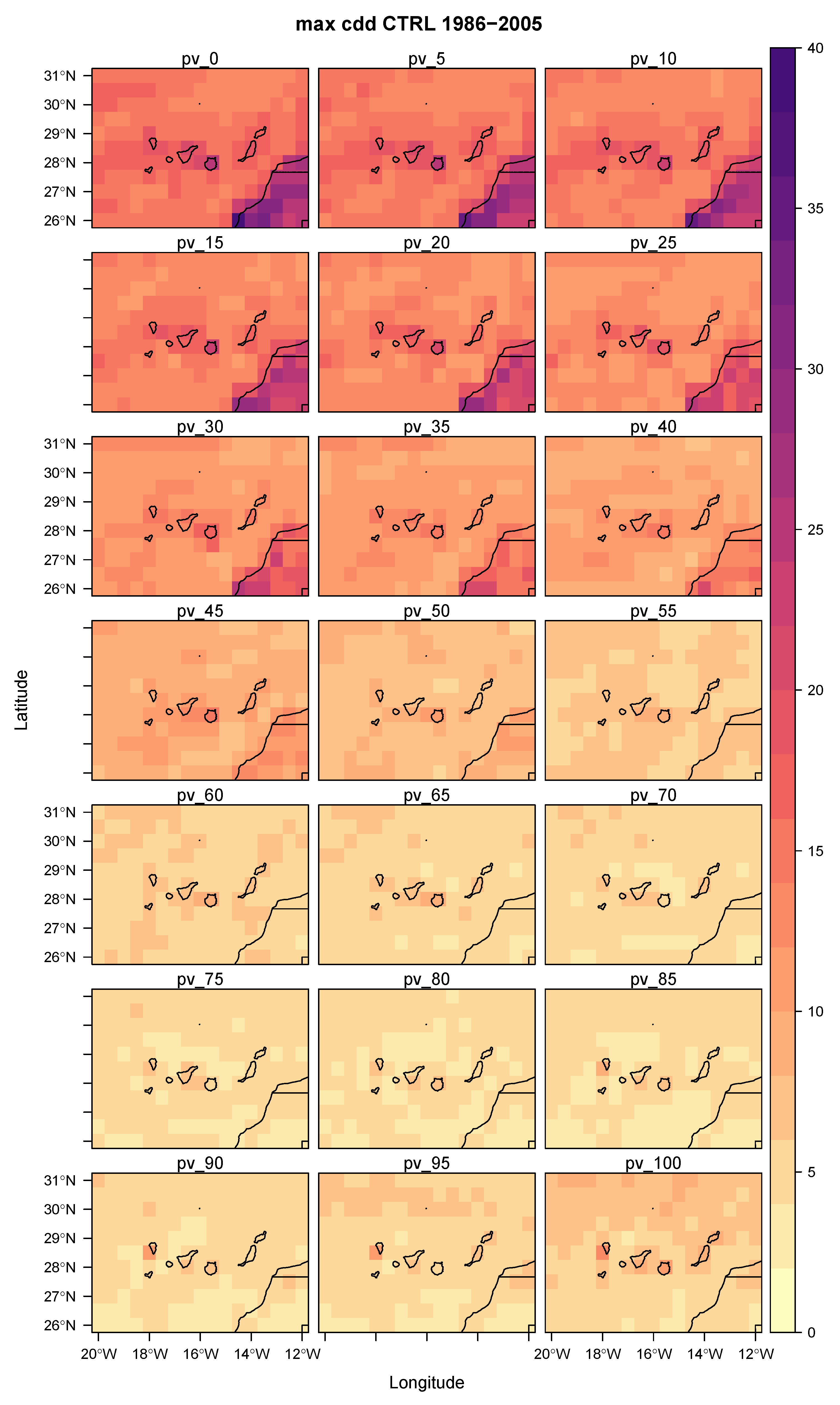
Figure A6.
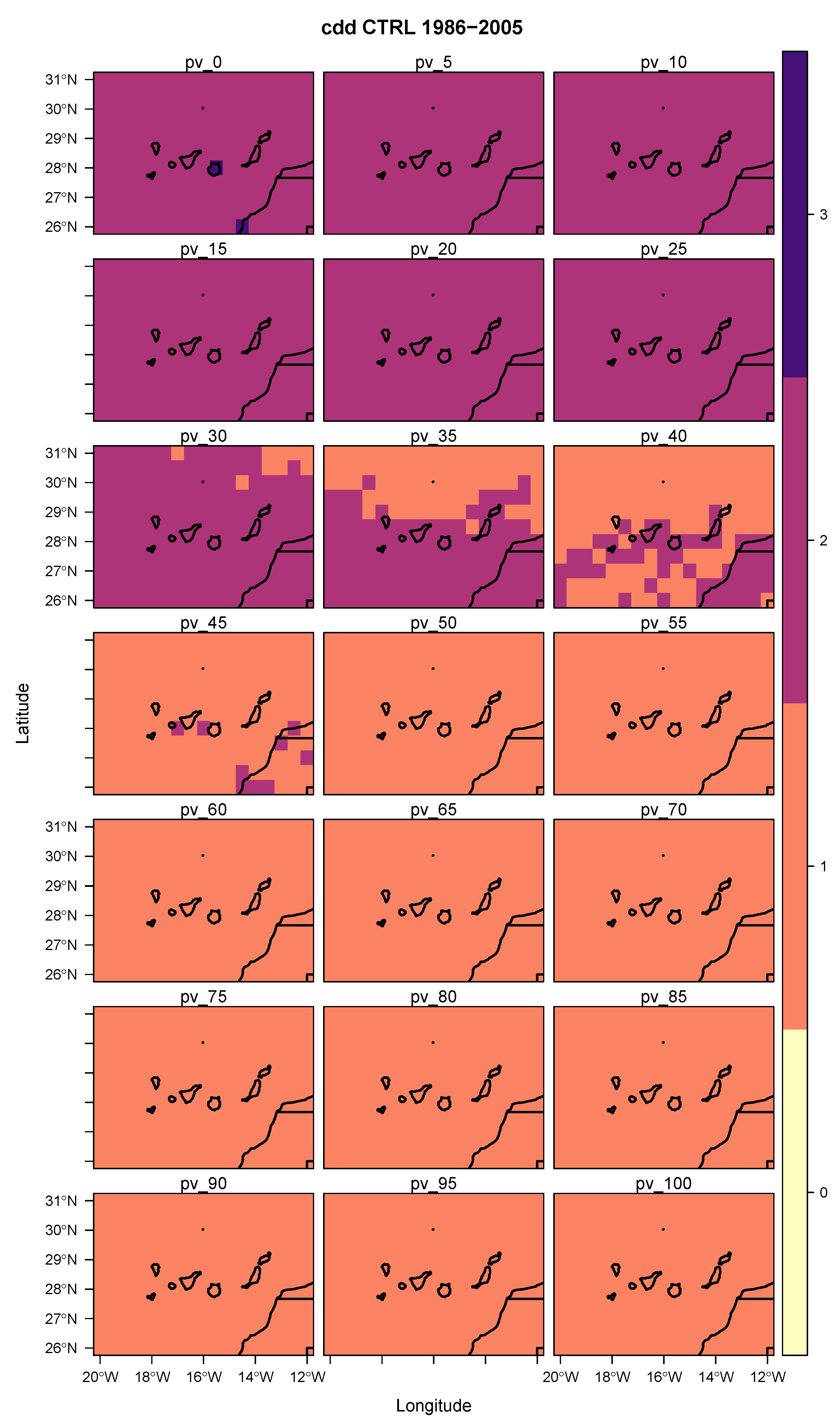
Maximum number of consecutive drought days, cdd, for the sensitivity analysis with different percentages of Spv (PV share) from 0 to 1 (from 0 to 100% of energy coming from PV), and the complementary wind energy share Sw.
Figure A6.
Maximum number of consecutive drought days, cdd, for the sensitivity analysis with different percentages of Spv (PV share) from 0 to 1 (from 0 to 100% of energy coming from PV), and the complementary wind energy share Sw.
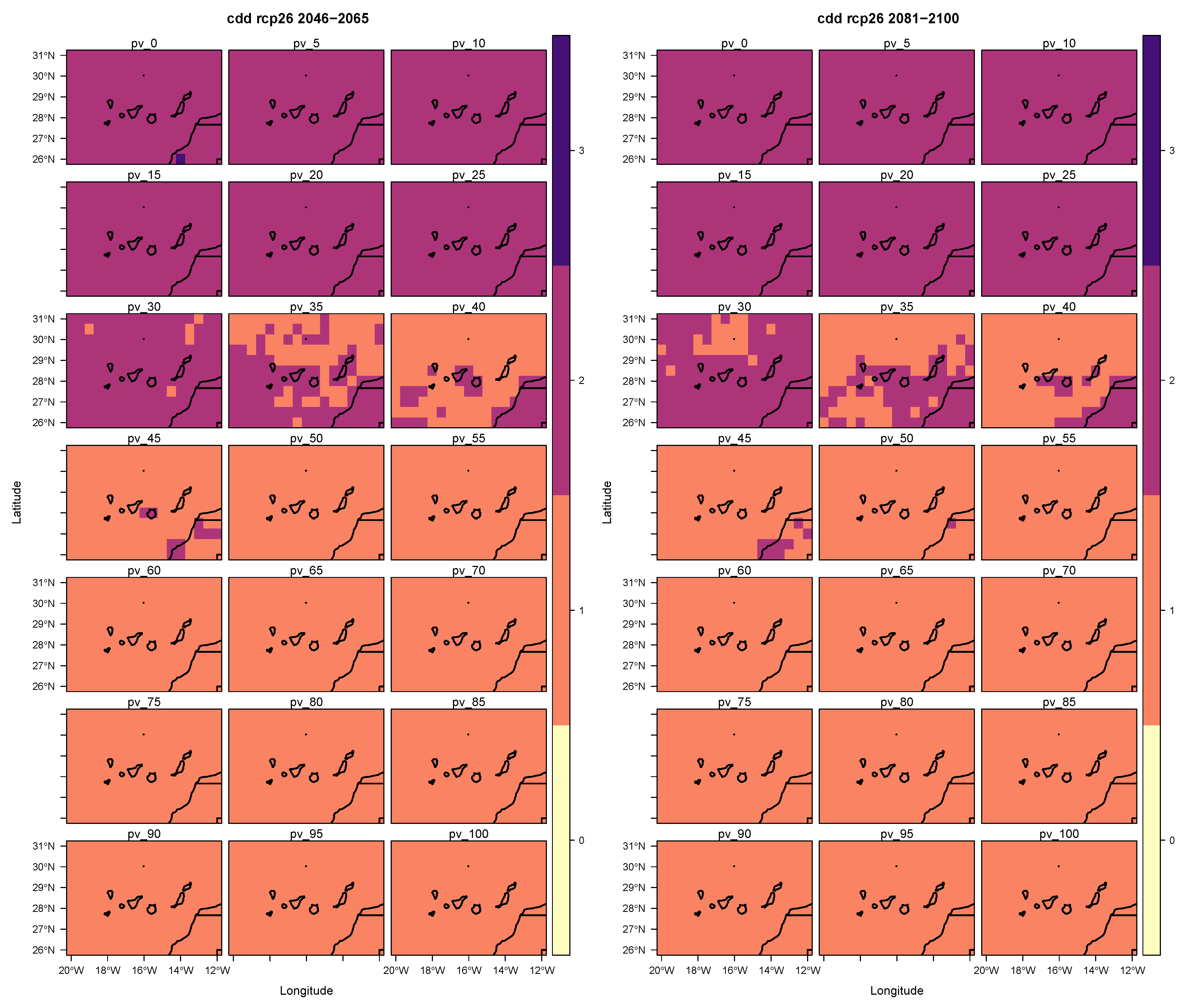
Figure A7.
As for
Figure A6 but for RCP2.6 scenario.
Left panel: 2046–2065 time period.
Right panel: 2081–2100 time period.
Figure A7.
As for
Figure A6 but for RCP2.6 scenario.
Left panel: 2046–2065 time period.
Right panel: 2081–2100 time period.
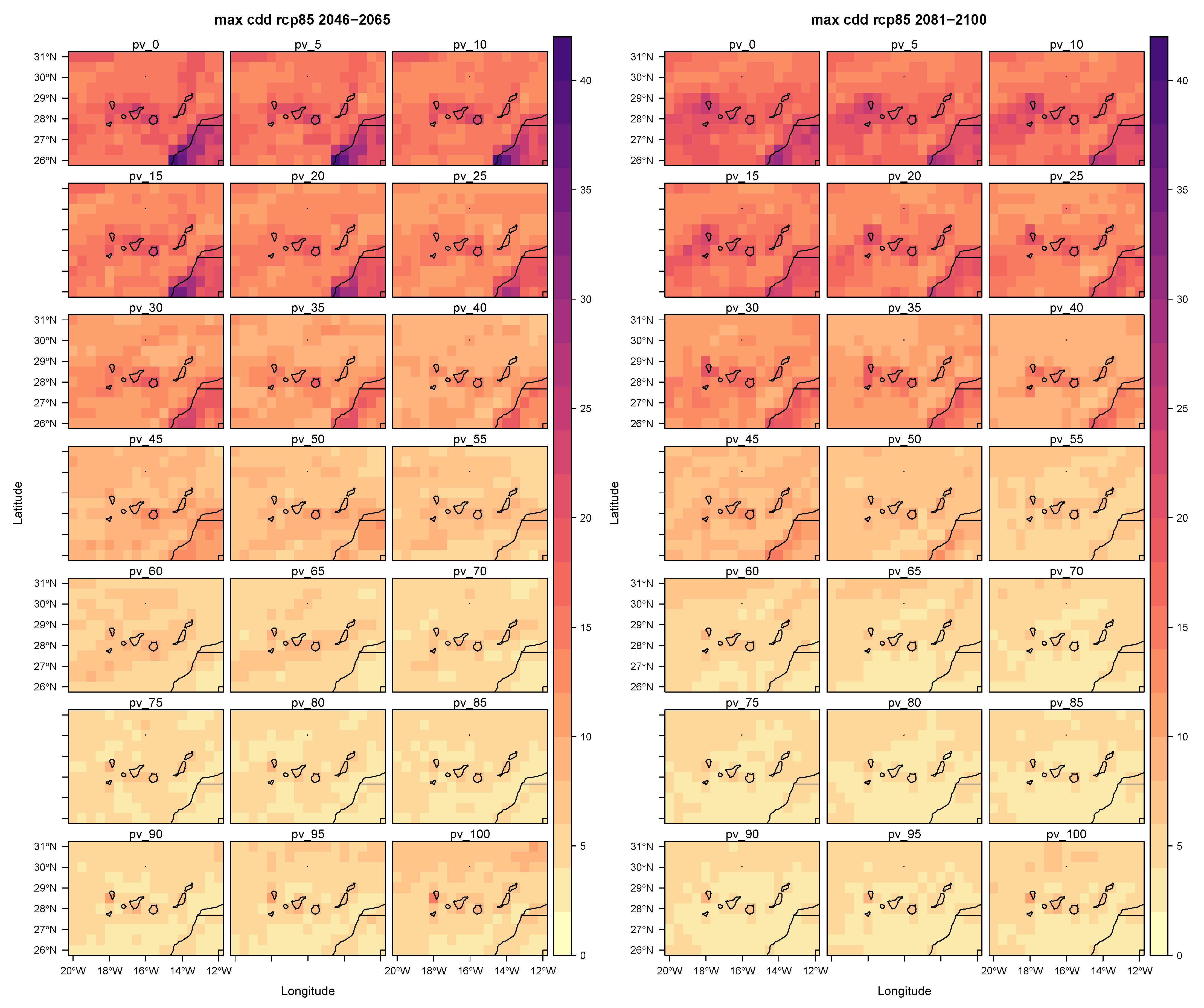
Figure A8.
As for
Figure A6 but for RCP8.5 scenario.
Left panel: 2046–2065 time period.
Right panel: 2081–2100 time period.
Figure A8.
As for
Figure A6 but for RCP8.5 scenario.
Left panel: 2046–2065 time period.
Right panel: 2081–2100 time period.
Figure A9.
Median value of consecutive drought days, cdd, for the sensitivity analysis with different percentages of Spv (PV share) from 0 to 1 (from 0 to 100% of energy coming from PV), and the complementary wind energy share Sw.
Figure A9.
Median value of consecutive drought days, cdd, for the sensitivity analysis with different percentages of Spv (PV share) from 0 to 1 (from 0 to 100% of energy coming from PV), and the complementary wind energy share Sw.
Figure A10.
As for
Figure A9 but for RCP2.6 scenario.
Left panel: 2046–2065 time period.
Right panel: 2081–2100 time period.
Figure A10.
As for
Figure A9 but for RCP2.6 scenario.
Left panel: 2046–2065 time period.
Right panel: 2081–2100 time period.
Figure A11.
As for
Figure A9 but for RCP8.5 scenario.
Left panel: 2046–2065 time period.
Right panel: 2081–2100 time period.
Figure A11.
As for
Figure A9 but for RCP8.5 scenario.
Left panel: 2046–2065 time period.
Right panel: 2081–2100 time period.
Figure A12.
As for
Figure 4, but this represents the value of Spv required to obtain the minimum p95 (wind and PV) of cdd (consecutive drought days) of the event. Panels (
A): Spv required to obtain the minimum p95 of combined (wind and PV) cdd. Panels (
B–
E): Future changes in Spv for the different time periods (2046–2065:
left column; 2081–2100:
right column) and scenarios (RCP2.6:
B,
C; RCP8.5:
D,
E). In panels B-E blue colors indicate a future increase of Spv and red colors the opposite. Panel (
F): This is equivalent to Panel A, but this shows the p95 of combined (wind and PV) cdd with the optimum value of Spv. Panels (
G–
J): These are equivalent to panels (
B–
E) but for the p95 of cdd with the optimum value of Spv.
References
- IPCC (United Nations). Fifth Assessment Report—Climate Change 2013; Technical Report; IPCC: Geneva, Switzerland, 2013. [Google Scholar]
- Schaeffer, R.; Szklo, A.S.; Pereira de Lucena, A.F.; Moreira Cesar Borba, B.S.; Pupo Nogueira, L.P.; Fleming, F.P.; Troccoli, A.; Harrison, M.; Boulahya, M.S. Energy sector vulnerability to climate change: A review. Energy 2012, 38, 1–2. [Google Scholar] [CrossRef]
- Bloomfield, H.C.; Brayshaw, D.J.; Shaffrey, L.C.; Coker, P.J.; Thornton, H.E. Quantifying the increasing sensitivity of power systems to climate variability. Environ. Res. Lett. 2016, 11, 124025. [Google Scholar] [CrossRef]
- Collins, S.; Deane, P.; Ó Gallachóir, B.; Pfenninger, S.; Staffell, I. Impacts of Inter-annual Wind and Solar Variations on the European Power System. Joule 2018, 2, 2076–2090. [Google Scholar] [CrossRef]
- Tobin, I.; Jerez, S.; Vautard, R.; Thais, F.; Van Meijgaard, E.; Prein, A.; Déqué, M.; Kotlarski, S.; Maule, C.F.; Nikulin, G.; et al. Climate change impacts on the power generation potential of a European mid-century wind farms scenario. Environ. Res. Lett. 2016, 11, 034013. [Google Scholar] [CrossRef]
- Karnauskas, K.B.; Lundquist, J.K.; Zhang, L. Southward shift of the global wind energy resource under high carbon dioxide emissions. Nat. Geosci. 2018, 11, 38–43. [Google Scholar] [CrossRef]
- Ciarlo, J.M.; Coppola, E.; Fantini, A.; Giorgi, F.; Gao, X.; Tong, Y.; Glazer, R.H.; Torres Alavez, J.A.; Sines, T.; Pichelli, E.; et al. A new spatially distributed added value index for regional climate models: The EURO-CORDEX and the CORDEX-CORE highest resolution ensembles. Clim. Dyn. 2020, 13, 1–22. [Google Scholar] [CrossRef]
- Renewables 2020 Global Status Report; Technical Report, REN21; IAEA: Paris, France, 2020.
- Panagea, I.S.; Tsanis, I.K.; Koutroulis, A.G.; Grillakis, M.G. Climate Change Impact on Photovoltaic Energy Output: The Case of Greece. Adv. Meteorol. 2014, 2014, 264506. [Google Scholar] [CrossRef]
- Jerez, S.; Tobin, I.; Vautard, R.; Montávez, J.P.; López-Romero, J.M.; Thais, F.; Bartok, B.; Christensen, O.B.; Colette, A.; Déqué, M.; et al. The impact of climate change on photovoltaic power generation in Europe. Nat. Commun. 2015, 6, 10014. [Google Scholar] [CrossRef]
- Jerez, S.; Thais, F.; Tobin, I.; Wild, M.; Colette, A.; Yiou, P.; Vautard, R. The CLIMIX model: A tool to create and evaluate spatially-resolved scenarios of photovoltaic and wind power development. Renew. Sustain. Energy Rev. 2015, 42, 1–15. [Google Scholar] [CrossRef]
- Tobin, I.; Vautard, R.; Balog, I.; Bréon, F.M.; Jerez, S.; Ruti, P.M.; Thais, F.; Vrac, M.; Yiou, P. Assessing climate change impacts on European wind energy from ENSEMBLES high-resolution climate projections. Clim. Chang. 2015, 128, 99–112. [Google Scholar] [CrossRef]
- Pérez, J.C.; González, A.; Díaz, J.P.; Expósito, F.J.; Felipe, J. Climate change impact on future photovoltaic resource potential in an orographically complex archipelago, the Canary Islands. Renew. Energy 2019, 133, 749–759. [Google Scholar] [CrossRef]
- Soares, P.M.; Lima, D.C.; Semedo, A.; Cardoso, R.M.; Cabos, W.; Sein, D.V. Assessing the climate change impact on the North African offshore surface wind and coastal low-level jet using coupled and uncoupled regional climate simulations. Clim. Dyn. 2019, 52, 7111–7132. [Google Scholar] [CrossRef]
- Soares, P.M.M.; Lima, D.C.A.; Semedo, A.; Cabos, W.; Sein, D.V. Climate change impact on Northwestern African offshore wind energy resources Climate change impact on Northwestern African offshore wind energy resources. Environ. Res. Lett. 2019, 14, 124065. [Google Scholar] [CrossRef]
- Jerez, S.; Tobin, I.; Turco, M.; Jiménez-Guerrero, P.; Vautard, R.; Montávez, J.P. Future changes, or lack thereof, in the temporal variability of the combined wind-plus-solar power production in Europe. Renew. Energy 2019, 139, 251–260. [Google Scholar] [CrossRef]
- Gutiérrez, C.; Somot, S.; Nabat, P.; Mallet, M.; Corre, L.; van Meijgaard, E.; Perpiñán, O.; Gaertner, M.Á. Future evolution of surface solar radiation and photovoltaic potential in Europe: Investigating the role of aerosols. Environ. Res. Lett. 2020, 15, 034035. [Google Scholar] [CrossRef]
- Global Energy Review 2020—Analysis—IEA; Technical Report; IEA: Paris, France, 2020.
- Kaldellis, J.K.; Kapsali, M. Shifting towards offshore wind energy-Recent activity and future development. Energy Policy 2013, 53, 136–148. [Google Scholar] [CrossRef]
- Lee, J.; Zhao, F. Global Wind Report 2019|Global Wind Energy Council; Technical Report; Global Wind Energy Council: Brussels, Belgium, 2019. [Google Scholar]
- Golroodbari, S.Z.; Sark, W. Simulation of performance differences between offshore and land-based photovoltaic systems. Prog. Photovolt. Res. Appl. 2020, 28, 873–886. [Google Scholar] [CrossRef]
- Witzke, U.; Cadamuro, M.; Aquilina, M.; Mule’Stagno, L.; Grech, M. Floating Photovoltaic Installations in the Maltese Sea Waters. In Proceedings of the 32nd European Photovoltaic Solar Energy Conference and Exhibition, Munich, Germany, 20–24 June 2016; pp. 1964–1968. [Google Scholar] [CrossRef]
- Buitendijk, M. Newly Installed Dutch Offshore Solar Farm Survives First Storms|SWZ|Maritime; SWZ|Maritime: Rotterdam, The Netherlands, 2019. [Google Scholar]
- WavEC: Combined Wind, Wave and Solar to Transform Marine Energy—Offshore Energy; WavEC: Lisbon, Portugal, 2019.
- SINN Power Supports MUSICA Project—Offshore Energy; SINN: Frankfurt, Germany, 2019.
- MaREI to Lead 9m Project to Build Floating Offshore Platform; MaREI: Cork, Ireland, 2019.
- Koletsis, I.; Kotroni, V.; Lagouvardos, K.; Soukissian, T. Assessment of offshore wind speed and power potential over the Mediterranean and the Black Seas under future climate changes. Renew. Sustain. Energy Rev. 2016, 60, 234–245. [Google Scholar] [CrossRef]
- Alvarez, I.; Lorenzo, M.N. Changes in offshore wind power potential over the Mediterranean Sea using CORDEX projections. Reg. Environ. Chang. 2019, 19, 79–88. [Google Scholar] [CrossRef]
- de la Vara, A.; Gutiérrez, C.; González-Alemán, J.J.; Gaertner, M.Á. Intercomparison Study of the Impact of Climate Change on Renewable Energy Indicators on the Mediterranean Islands. Atmosphere 2020, 11, 1036. [Google Scholar] [CrossRef]
- Wind Energy in Spain: First Offshore Wind Farm Project|REVE News of the Wind Sector in Spain and in the World; REVE News: Madrid, Spain, 2001.
- Almazroui, M. Temperature Changes over the CORDEX-MENA Domain in the 21st Century Using CMIP5 Data Downscaled with RegCM4: A Focus on the Arabian Peninsula. Adv. Meteorol. 2019, 2019, 5395676. [Google Scholar] [CrossRef]
- Raynaud, D.; Hingray, B.; François, B.; Creutin, J.D. Energy droughts from variable renewable energy sources in European climates. Renew. Energy 2018, 125, 578–589. [Google Scholar] [CrossRef]
- Elliott, D.; Holladay, C.; Barchet, W.; Foote, H.; Sandusky, W. Wind Energy Resource Atlas of the United States; NASA STI/Recon Technical Report N 87; Pacific Northwest Lab.: Richland, WA, USA, 1987.
- Gutiérrez, C.; Somot, S.; Nabat, P.; Mallet, M.; Gaertner, M.Á.; Perpiñán, O. Impact of aerosols on the spatiotemporal variability of photovoltaic energy production in the Euro-Mediterranean area. Sol. Energy 2018, 174, 1142–1152. [Google Scholar] [CrossRef]
- Liu, B.Y.; Jordan, R.C. The interrelationship and characteristic distribution of direct, diffuse and total solar radiation. Sol. Energy 1960, 4, 1–19. [Google Scholar] [CrossRef]
- Collares-Pereira, M.; Rabl, A. The average distribution of solar radiation-correlations between diffuse and hemispherical and between daily and hourly insolation values. Sol. Energy 1979, 22, 155–164. [Google Scholar] [CrossRef]
- Hay, J.E.; McKAY, D.C. Estimating solar irradiance on inclined surfaces: A review and assessment of methodologies. Int. J. Sol. Energy 1985, 3, 203–240. [Google Scholar] [CrossRef]
- Gutiérrez, C.; Gaertner, M.Á.; Perpiñán, O.; Gallardo, C.; Sánchez, E. A multi-step scheme for spatial analysis of solar and photovoltaic production variability and complementarity. Sol. Energy 2017, 158, 100–116. [Google Scholar] [CrossRef]
- Perpiñan, O. Statistical analysis of the performance and simulation of a two-axis tracking PV system. Sol. Energy 2009, 83, 2074–2085. [Google Scholar] [CrossRef]
- R Core Team. R: A Language and Environment for Statistical Computing; R Foundation for Statistical Computing: Vienna, Austria, 2020. [Google Scholar]
- Perpiñán, O. solaR: Solar Radiation and Photovoltaic Systems with R. J. Stat. Softw. 2012, 50, 1–32. [Google Scholar] [CrossRef]
- Perpiñán, O.; Hijmans, R. rasterVis, R Package Version 0.50.1; R Package: Madison, WI, USA, 2021. [Google Scholar]
- François, B.; Borga, M.; Creutin, J.D.; Hingray, B.; Raynaud, D.; Sauterleute, J.F. Complementarity between solar and hydro power: Sensitivity study to climate characteristics in Northern-Italy. Renew. Energy 2016, 86, 543–553. [Google Scholar] [CrossRef]
- de Oliveira Costa Souza Rosa, C.; Costa, K.; da Silva Christo, E.; Braga Bertahone, P. Complementarity of Hydro, Photovoltaic, and Wind Power in Rio de Janeiro State. Sustainability 2017, 9, 1130. [Google Scholar] [CrossRef]
- de Oliveira Costa Souza Rosa, C.; da Silva Christo, E.; Costa, K.A.; dos Santos, L. Assessing complementarity and optimising the combination of intermittent renewable energy sources using ground measurements. J. Clean. Prod. 2020, 258, 120946. [Google Scholar] [CrossRef]
- Odeh, R.P.; Watts, D.; Flores, Y. Planning in a changing environment: Applications of portfolio optimisation to deal with risk in the electricity sector. Renew. Sustain. Energy Rev. 2018, 82, 3808–3823. [Google Scholar] [CrossRef]
- Lehmann, P.; Söderholm, P. Can technology-specific deployment policies be cost-effective? The case of renewable energy support schemes. Environ. Resour. Econ. 2018, 71, 475–505. [Google Scholar] [CrossRef]
- International Renewable Energy Agency. Renewable Energy Auctions: Status and Trends beyond Price; International Renewable Energy Agency: Abu Dhabi, United Arab Emirates, 2019. [Google Scholar]
| Publisher’s Note: MDPI stays neutral with regard to jurisdictional claims in published maps and institutional affiliations. |
© 2021 by the authors. Licensee MDPI, Basel, Switzerland. This article is an open access article distributed under the terms and conditions of the Creative Commons Attribution (CC BY) license (https://creativecommons.org/licenses/by/4.0/).


 ,
, 


