Assessment of State Transition Dynamics of Coastal Wetlands in Northern Venice Lagoon, Italy

Abstract

Coastal wetlands represent particularly valuable natural resources, characterized by the interaction between their geomorphological and biological components. Their adaptation to the changing conditions depends on the rate and extent of spatial and temporal processes and their response is still not fully understood. This work aims at detecting and improving the understanding of the transition dynamics on eco-geomorphological structures in a coastal wetland ecosystem. The approach could support sustainable habitat management improving the detection and optimizing the offer of Earth Observation (EO) products for coastal system monitoring. Such course of action will strengthen evidence-based policy making, surface biophysical data sovereignty and the Space Data downstream sector through remote sensing techniques thanks to the capability of investigating larger scale and short-to-long-term dynamics. The selected case study is the Lido basin (Venice Lagoon, Italy). Our methodology offers a support in the framework of nature-based solutions, allowing the identification of ecosystem-level indicators of the surface biophysical properties influencing stability and evolution of intertidal flats on which a conceptual model is implemented. Landsat satellite imagery is used to delineate the spatial and temporal variability of the main vegetation and sediment typologies in 1990–2011. Within this period, specific anthropic activities were carried out for morphological restoration and flood protection interventions. Specifically, the lower saltmarsh shows its more fragmented part in the Baccan islet, a residual sandy spit in front of the Lido inlet. The area covered by Sarcocornia-Limonium, that triggers sediment deposition, has fluctuated yearly, from a minimum coverage of 13% to a maximum of 50%. The second decade (2001–2009) is identified as the period with major changes of halophytic and Algae-Biofilm cover typologies distribution. The power law and related thresholds, representing the patch size frequency distribution, is an indicator of the ecosystem state transition dynamics. The approach, based on multi-temporal and spatial EO analysis, is scalable elsewhere, from regional to local-to-global scale, considering the variability of climate data and anthropogenic activities. The present research also supports sustainable habitat management, improving the detection, and optimizing the offer of EO products for coastal system monitoring.

1. Introduction

Coastal wetlands represent complex ecosystems prone to continuous changes. These changes are especially standing out nowadays due to the existing feedback loop between the impact of climate change and anthropic activities, ecosystem degradation, and the increased risk of natural disaster.

The morphological change of land processes can be fully understood as long as all the significant interactions between the physical and biological components are considered [1,2,3,4,5,6]. The role of the eco-geomorphological responses caused by the interaction between biotic and abiotic processes (e.g., vegetation growth, sedimentary processes, microphytobenthos influences, waves, tides or storm surges), has been recently recognized [7,8,9,10,11,12,13], leading to the development of new approaches. Special emphasis is given to bio-geophysical processes when studying the change of intertidal landscapes [3,4,14].

Intertidal mudflats are fine sediment deposits that are periodically submerged during the high tide. Mudflats have a worldwide distribution. They are ephemeral on a geological time-scale (they last a few thousand years), but have a fundamental ecological role and are characterized by extremely high biological productivity, which plays an important role in the balance between marine and terrestrial ecosystems [15,16]. Due to intermittent flooding and exposure to the atmosphere, they are characterized by many different physical and biological processes that can influence their composition and habitats [17,18,19]. Generally, they are composed of coarser sediment in the subtidal areas (below the low tide level) and finer sediments in the upper part (between the mid and the high tide levels). Mudflats are classified according to the tidal range, wave energy, sediment supply, morphology, physical and biological properties [20]. The tidal range is one of the most important parameters for the classification because of its role in controlling bed morphology. However, the sedimentological, biological, and oceanographical characteristics of mudflats still need to be deeply understood [21].

Lagoons’ ecosystems are represented by low-elevation bare flats and upper vegetated saltmarshes. These components are constantly interacting [22] and are thereby prone to continuous changes of their internal equilibrium. Vegetation’s spatial distribution stands out for its complex patterns and striking features. Particularly in saltmarshes, given the self-organization in patchy distributions [13,23,24,25,26,27,28], a key role in ecological stability and disturbance-recovery processes has been observed [29,30,31,32]. In spatially organized ecosystems, the patchiness can be generated by a wide variety of dynamics. Identifying the way vegetation, substrates and waters are distributed and organized, as well as the manner of change under the influence of the surrounding environment, provides valuable information to deduce the system’s behavior and predict its spatial dynamics. On the other hand, eco-geomorphological dynamics of saltmarshes are strongly influenced by the wide range of spatial scales of the changing processes, from few centimeters to several kilometers.

External forces cannot explain solely the status of ecosystems but can influence the spatial bio-geomorphological structure organization. Accordingly, ecosystem- or landscape-level indicators are being continuously developed as a manageable set of indicators that reflects the structural and functional properties of the landscape units (i.e., effects of anthropogenic and environmental disturbances) [33]. For instance, the self-organized patchiness of sediments and vegetation is often used as an indication of ecosystem stability and dynamics [28].

The way in which spatial patterns reflects the level of disturbances exerted on the ecosystem and thereby its level of stability can be used to understand whether self-organization induces stability in ecosystems or pushes ecosystems towards the edge of collapse [29,34,35,36]. The elevation of sediment banks from subtidal to intertidal levels is the first step to trigger bio-stabilization and colonization of pioneering vegetation. The competent authorities started to adopt more practical but scientific-based solutions, demonstrating the important role of mudflat morphology (elevation and time of exposure) on bio-stabilization processes and its effect on the resilience and development of intertidal areas within the Venice Lagoon [18,19,37].

The advantage of reducing mudflats erosion, other than habitat conservation, is to lower sedimentation in the natural channels, and remote sensing provides a defense model for detecting sediment erosion. Nowadays, the opportunities offered by the synergies between traditional and innovative remote sensing platforms (e.g., satellites and drones) allow the near real-time monitoring of natural and human-induced changes in tidal flows. The blended monitoring approach (traditional with innovative) allows expanding the model to a variety of complex systems, from marine to marine-coastal (subtidal belt) and transitional (intertidal belt) systems, each subject to different prevailing external forcing.

Complex systems, where small-scale interactions scale up to large-scale changes, are characterized by a range of small and large patches that determines the spatial structure of the system. The Power Law Distribution (PLD), a statistical indication of the scale-dependent distributions, offers a unique tool to explore physical mechanisms and self-organization of sediments and vegetation spatial patterns [38,39,40]. Particularly, PLD of patch sizes can be interpreted as a sign of self-organization and it allows characterizing the spatial processes occurring at the boundary of the existing patches, determined by their spatial extension or contraction [27,30,41,42].

According to recent studies [40,43,44], it is fundamental to understand the non-linear dynamics observed in the power law tail, whereas the deviation in the patches’ size distribution is crucial to forecast the system response to environmental changes. It evidences the tuning of morphological restoration (mudflat-saltmarsh anthropogenic reconstruction) to the subsequent complex feedbacks between the vegetation-sediment distribution and external drivers. Recent studies in lake systems, oceans, and forests show how the gradual change is in some cases interrupted by sudden changes that determine the transition to a new state, when a threshold value in environmental conditions is exceeded [45].

Temporal trends’ characterization, as extent and size of patches’ patterns, is further fundamental to discriminate the changes in both space and time directions. The Empirical Orthogonal Function (EOF) [26] is a valuable tool, largely used in climatology, oceanography, and Earth Observation (EO) disciplines to rank spatial patterns of variability, their time variation and the importance of each pattern on the basis of variance [46]. Particularly, it allows to isolate the major phases of changes through the EOFs’ expansion coefficients along the time series and to assign a measure of the importance of each pattern.

The integration of field observations and quantitative tools, such as Earth Observation (EO) enable an accurate insight into the wide range of spatial scales and mechanisms. Satellite remote sensing allows accurate and repeatable data acquisitions over large areas [8,14,47,48,49,50], therefore, it is a key data source, especially due to nowadays with easy access to open satellite data [51,52]. Given the fact that small perturbations cause the instability of the system and rapid changes in the landscape, EO is an interesting tool to study the scale variance and invariance of bio-geomorphological process [27,32,52,53,54,55,56,57,58].

EO-based studies can highlight the conditions under which variations in patch size distributions are important determinants, e.g., for animals living in patchy intertidal landscapes like many migratory and non-migratory ornithic species [50,59]. Adaptation in the species’ population size may occur responding to habitat loss (e.g., reclamation or flood) and to human recreational or productive activities. Seasonal hydrologic variability, as well as artificially induced water-level fluctuations, has been proven to threaten the reproductive success of some bird species in different climatic zones of the world [60]. Tidal flats are significantly impacted by rising sea levels and intensifying storms under climate change [61]. For example, given that most tidal flats in the Yellow Sea are bounded by rock walls and coastal development, ecosystem migration in response to rising sea levels cannot occur, which lead to inundation of the ecosystem, reducing the key process of regular tidal inundation, changes in distribution and declines in extent [62]. Therefore, the spatial and temporal trends of changes in intertidal areas within a lagoon can be fundamental for conservation and resilience studies [63].

This paper presents a comprehensive method developed through the analysis of multi-source open data applied to a shallow tidal basin of saltmarshes and mudflats in the Northern part of the Venice Lagoon (North-East of Italy), the Lido basin. The research questions addressed are built on the conceptual model of mudflats and their transition dynamics, and have the goal to improve the understanding of eco-geomorphological structure changes using vegetation and biofilm cover classes. The spatial structure dynamics and the way spatial patterns manifest themselves over time (i.e., the PLD and the EOF analyses) are used to detect the influence of external drivers. In the study area, particular emphasis has been given to bio-stabilization processes linked to morphological restoration as a major thematic area. The spatial and temporal ecosystem-level indicators allow identifying which kind of processes influence the behavior of the spatial structures’ response to environmental changes, leading to possible evidence of criticalities.

This is the base for sustainable management policies driven by the adoption of nature-based solutions. Using tradeoffs between exploitation and conservation, especially for utilization of sediment, water and biological resources, is key to guaranteeing the maintenance of ecosystem services provision.

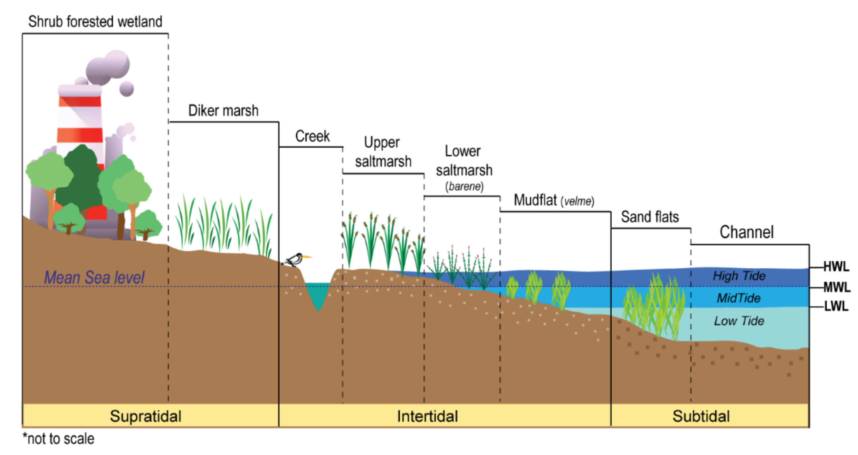
2. Study Area: The Lido Basin in the Venice Lagoon

The study area is in one of the most valuable coastal transitional ecosystems in the Mediterranean Sea: The Venice Lagoon. The Lagoon is suffering of ecosystem degradation. It is located along the North-Western coastline of the Adriatic Sea, bounded by the Sile River to the North and the Brenta River to the South. It is connected to the sea by three inlets of 500 m to 900 m wide and to 15 m deep. Venice Lagoon is divided into three basins, named after the inlets: Lido in the North (276 km²), Malamocco in the middle (112 km²) and Chioggia in the South (111 km²).

The Lagoon is the largest wetland in Italy, with a surface of 550 km² (

Table 1. Main morphological categories in Venice Lagoon, their bathymetry and distribution (adapted from [65]).

Morphological Categories	Bathymetry (m)	Surface (km2)
Islands	>0.5	100
Intertidal marshes	from 0.0 to 0.5	30
Intertidal flats	from −0.3 to 0.0	40
Shallow areas	from −2.0 to −0.3	230
Channels	<−2.0	60
Fish farms	-	90

). Venice Lagoon is a microtidal environment in which the neap tide is 30 cm, the mean tide is 55 cm and the spring tide is 110 cm [19]. Tidal waves are semidiurnal and asymmetric in form. Two high tides (HWL) and low tides (LWL) occur every day. HWL are increased by Scirocco wind, low atmospheric pressure and river discharge. Acqua Alta events can increase the HWL (~1 m) during spring tides and southerly winds. The maximum HWL reached up to 192 cm on 4 November 1966. Tidal wave is slowed down when entering the Lagoon and propagates within the Lagoon different delays. The tide height is also lowered within the Lagoon due to the friction exerted by the bottom [64].

The complexity of its landscape results from the interaction between natural processes and human interventions. Human activities have modified the environment of the Lagoon in several ways during the last five centuries. A drastic change has occurred in the hydrological regime of the rivers flowing into the Lagoon. This modern morphology has been created by a variety of human activities, also during the Anthropocene, and is classified into six categories (Table 1).

During the time interval considered in the present study (two decades between 1990–2011), several interventions were carried out within the Venice Lagoon as part of a Morphological Master Plan of the Consorzio Venezia Nuova (CVN). Since the 1990s, several dredging and saltmarsh restoration were carried out. In the Northern part of the Venice Lagoon, saltmarsh restoration was carried out in the period between 2000 and 2002. Then, since 2007, the realization of hard infrastructures at the three inlets for the Lagoon took place.

The study area has thus been always subject to natural siltation mitigated by different types of anthropogenic interventions such as dredging, protection against high water, river diversion, and morphological restoration [66]. Recently, the Experimental Electromechanical Module (MOSE) project was installed across the three inlets that link the Lagoon to the Adriatic Sea, to protect the city of Venice from flooding [67]. The mobile barriers consist of 79 elements placed perpendicularly to the main three inlets and represent a significant anthropogenic structure that influence the hydrodynamics, sediment transport, and the habitat distribution of the Lagoon [67,68].

The MOSE project has been designed to protect the city of Venice against the Acqua Alta phenomenon, but during its construction, the winter seasons in 2008–2010 were characterized by numerous episodes of high tide and heavy rainfall. 2008–2010 is characterized as anomalous in comparison to the last 30 years and this change in the frequency of inundation led to eco-morphological changes.

The selected case study (16 km²) is within the Lido basin, represented by temporarily exposed mudbanks and barene and velme (local name for the saltmarshes and mudflats) (Figure 1). The basin (276 km²; 50% of Venice Lagoon surface) comprises the islet of Baccan (a residual sandy spit) and part of the San Felice marshy wetlands, incised by meandering tidal networks.

Venice Lagoon shows unique ecological characteristics at a national level and in the context of the Mediterranean basin. In fact, it is included in the list of wetlands of international importance [69] and the European Community, with the financial instrument for the environment (LIFE), is granting a wide variety of funds for nature conservation and restoration programs.

Venice Lagoon is regulated by special laws, thereby defining a benchmark for pioneering legislation of coastal sustainable development to balance anthropogenic impact and natural capital conservation. The Lido basin area was selected because of its ecological and biological value in terms of habitat conservation. The Northern part of the Venice Lagoon holds several listed habitats of the Habitats and the Birds Directives (1992/43/EEC and 2009/147/EEC). In addition, the Directive 2000/60/EC of the European Parliament and of the Council, establishes a Framework for Community Action in the Field of Water Policy to protect aquatic environments by making it compulsory to achieve a good environmental status for the coastal waters. In Italy, a series of bioindicator species have been selected to establish the ecological status of marine systems.

Mainly halophytic species colonized the basin, e.g., Spartina maritima, Salicornia veneta, Limonium narbonense, Sarcocornia fruticosa, and Juncus spp. [8,47]. The continuous changes in the sediment stability of the Northern Adriatic wetland system have led to fluctuations of the population of migratory ornithic species, such as the Little Tern (Sterna albifrons Pallas). Italy hosts the largest population in Europe of the Little Tern and about 85% of the population lives along the coast of the Northern Adriatic. Specifically, a post-breeding colony of thousands of individuals have historically sited in the Venice Lagoon between mid-June and early September, in correspondence to the existence of an intertidal sandy bar that is not submerged during the average tide [19,50].

The glossary used to describe the coastal tidal system metrics in the following sections is graphically displayed in Figure 2.

2.1. Climate Settings

Climate contributes to the unusualness of the landscape and biodiversity of the Venice Lagoon. The Northern Adriatic is a slightly more humid sector than usual in the Mediterranean Sea as a transition between the Mediterranean and the Atlantic climate conditions. Data obtained for the Cavallino (Treporti) station (ISPRA service for the Venice Lagoon) show that precipitation peaks characterize the study area in spring and autumn. Higher values are obtained in September and October (98–104 mm) and lower from January to March (42–49 mm). The annual mean temperature is 14 °C, with a relatively hot and humid summer (

Table 2. The monthly cumulative precipitation (P) and the monthly temperature (T) in Venice Lagoon. Data obtained for the Cavallino (Treporti) station for the period of 1990–2011. Source: Italian Institute for Environmental Protection and Research (ISPRA), freely available online [70].

Parameters	Monthly Mean												Annual Mean
	J	F	M	A	M	J	J	A	S	O	N	D
T (°C)	3.80	4.73	8.30	12.49	17.75	21.24	23.42	23.56	19.18	14.65	9.27	4.76	13.59
P (mm)	42.40	47.86	48.93	74.48	72.63	64.81	57.03	72.55	103.79	98.12	90.30	72.62	70.46

) [70].

2.2. Characterization of Dominant Processes

Tides and winds (Bora and Scirocco, from the North- and South-East, respectively) are the main driving forces that affect the hydrological and sedimentary dynamics of the Lagoon [71,72]. Land subsidence also contributes to the elevation loss with respect to the mean sea level. In fact, most of the Northern Adriatic coastland lays below the mean sea level. Ground displacements of this coastland are caused by the individual and/or combined action of natural and anthropogenic factors (i.e., eustacy and groundwater pumping, respectively). In the Northern sector of the Venice Lagoon, this process continues with sinking rate on saltmarshes and intertidal environments ranging from 5 to 10 mm/year [73,74]. The short-term sedimentation and surface elevation change of wetlands in the Lagoon are due to changing water levels which have been measured at several stations with varying sediment input/availability and wave energy [75].

Mainly medium-fine sediments compose the Lagoon: silty sand, sandy silt, and silt. The grain size distribution reflects the environmental hydrodynamic energy. The coarsest sediments (sands) are distributed along the inlets and main tidal channels [19]. Both the tidal regime and the wave action reach their maximum in these areas, where sediment transportation is based on traction, rolling, and saltation. Instead, the finer sediments (silts and clays) concentrate along the inland areas, where a low flow energy deposits the fine matter that remained suspended in the water [76].

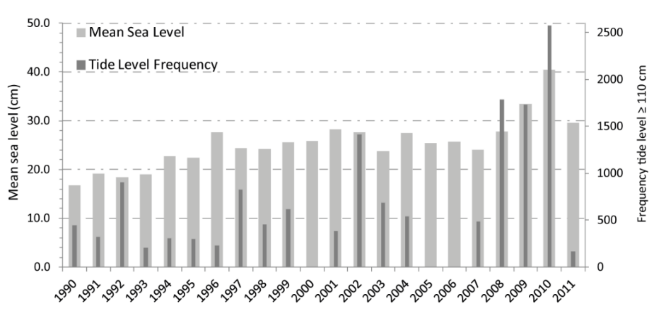
2.3. Characterization of Tidal Regime

The environment of the Lagoon is characterized by the tidal forcing with a first harmonic at 12 h with an average tidal range of about 60 cm, and about 1 m excursion in spring. The tide propagates along the deep narrow channels onto the tidal flats and tidal marshes [77]. The frequency distribution of high-extreme tide levels over 110 cm increased in the last decade, especially in 2008–2010. In the same period, Venice Lagoon was affected by the highest mean sea level, which reached 40.5 cm in 2010 (Figure 3). This value lays into the highest observed in the last 120 years [70].

3. Materials and Methods

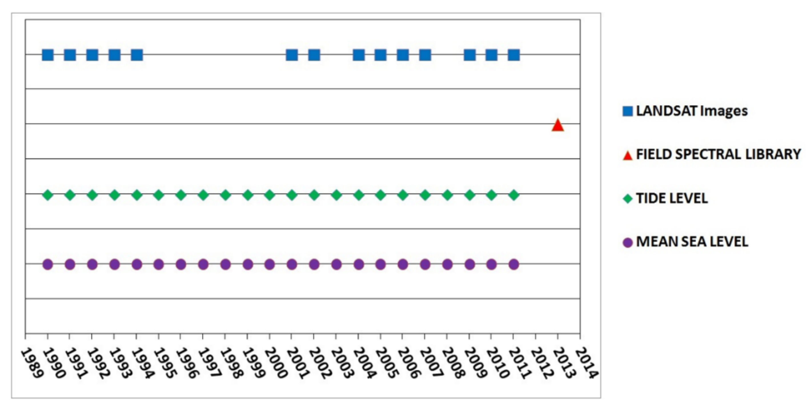
3.1. Materials

The developed methodology required different kind of inputs, namely EO data, field spectral data, and the annual tide level and mean sea level for the period of 1990–2011 (Figure 4). From the United States Geological Survey Earth Explorer, 18 cloud-free Landsat images (level 1T, Top-Of-Atmosphere radiance) covering the period 1991–2011 were acquired. The images are acquired by the Landsat-4, Landsat-5, and Landsat-7 satellite platforms (

Table A1. Landsat satellite data acquired for the period of 1990–2011: date, sensor, path, row, and tide level (cm).

Acquisition	Sensor	Path	Row	Tide Level (cm)
25/06/1990	TM	192	28	11.3
30/07/1991	TM	192	28	21.0
09/08/1992	TM	192	28	21.0
04/07/1993	TM	191	29	6.7
14/07/1994	TM	192	28	12.7
03/08/2001	ETM+	191	29	25.5
18/05/2002	ETM+	191	29	22.0
27/06/2002	TM	191	29	18.7
07/06/2004	TM	192	28	30.8
29/07/2005	ETM+	191	28	31.3
10/09/2006	TM	191	29	13.8
12/10/2006	TM	191	29	28.2
24/05/2007	TM	191	29	30.3
27/07/2007	TM	191	29	32.3
14/06/2009	TM	191	29	34.4
16/07/2009	TM	191	29	24.0
03/07/2010	TM	191	29	28.4
22/07/2011	TM	191	29	39.0

) and since 1995–2000, 2003, and 2008, lack of good quality images for the June–August period of interest, and just the other years in the period of 1990–2011 are included in the satellite data series.

The selected images for the case study are those preferably captured in July due to the higher vegetation vigorousness. With a pixel spatial resolution of 30 × 30 m, the entire surface selected as study area is about 15.804 km². The processed data cube has an extent of 17,560 pixels in terms of surface and it is made by a stack of 108 layers of information (18 dates × 6 spectral bands each) for a total of 1,896,480 cells. Values of the tide level, recorded at the EO images acquisition time (Table A1), are used to represent the transition between the permanently emerged and submerged environment to mask the extension of the analysis. This allows avoiding detecting spatiotemporal variations that rely on tidal fluctuations, thereby reducing uncertainties.

The field spectral library has been collected in June 2013 to validate the spectral endmembers selected on the EO imagery and to characterize the main sediment, biofilm and vegetation cover and the mixtures of them (Figure 1).

3.2. Methodology

The implementation of tools for monitoring for sustainable development need to detect variables in the spatial and temporal dimensions. The methodology proposed to identify ecosystem-level indicators for state transition dynamics in the case study consists of two main processes: (i) image field-based analysis (Linear Spectral Mixture Analysis, LSMA), based on cover typologies classification and validation using field spectral sampling [53], and (ii) a spatiotemporal analysis applying the EOF and the PLD [27] (Figure 5).

3.2.1. Image Field-Based Analysis

The image field-based analysis includes a sub-pixel processing technique, i.e., the Linear Spectral Mixture Analysis (LSMA), to obtain the spatial distribution of vegetation typologies and different wet and dry sediment transitions. The selection of the endmembers, one of the main phases of LSMA process to achieve cover fractional abundance maps at a pixel level (30 × 30 m in the case study with the Landsat images), is validated using the spectral library obtained by field radiometry.

Field campaigns are performed for better understanding the sediments’ variability, considering the influence of the biofilms covering the tidal bare substrates, and to collect the spectral library used to classify the vegetation typologies and validate the endmember collection [50,53].

The field spectral library acquired in June 2013 identifies the main vegetation and sediment typologies, e.g., Sarcocornia, Limonium, Juncus, and Algae-Biofilm. First, the field spectral library is resampled to the Landsat satellite spectral resolution. Then, it is compared with the spectral signatures of the vegetation and sediment endmembers previously selected. Subsequently, the field spectral signatures are used to simulate a reflectance spectrum (ρ(λ)_linear) as similar as possible to the reference spectral profile of the selected endmembers, according to Equation (1).

This equation was based on finding a linear relation between the reflectance values of the field spectral signature of each endmember (${\rho }_{e{m}_n}$) and the equivalent endmember percentage ($f_{e{m}_n}$). The difference (Δρ(λ)) between the simulated spectral signature (ρ(λ)₀) and the reference one (ρ(λ)linear) must be as minimum as possible (Equation (2)).

$$\rho \left(\lambda \right)linear=\rho {\left(\lambda \right)}_{em1} \times f_{em1}+\rho {\left(\lambda \right)}_{em2} \times f_{em2}+ \rho {\left(\lambda \right)}_{e{m}_n} \times f_{e{m}_n}$$

(1)

$$\Delta \rho \left(\lambda \right)= \rho {\left(\lambda \right)}_0-\rho {\left(\lambda \right)}_{linear}$$

(2)

To achieve this goal, the Microsoft Excel Solver was used. This tool allows finding the values of certain cells in a spreadsheet that optimize (maximize or minimize) a certain objective. Thus, the optimization model comprises three components:

• The target cell: the goal to achieve. In this case, obtaining the minimum difference (Δρ(λ)) between the simulated spectral signature (ρ(λ)0) and the reference one (ρ(λ)_linear).
• The changing cells: the cells of the spreadsheet that can be adjusted to optimize the target cell. In this case, the endmember fraction ($f_{e{m}_n}$).
• The constraints: the restrictions placed on the changing cells.

3.2.2. Spatiotemporal Analysis

The main aim of analyzing the spatiotemporal trends of this coastal wetland is identifying the tipping points that are likely inducible to a critical state, as well as the main climatic, hydrodynamic, and morphological variables that influence and intensify this behavior.

Then, the permanently emerged areas, characterized by the presence of the four cover typologies, were assayed by means of its temporal, i.e., the EOF, and spatial, i.e., the PLD, distribution in order to characterize the variation trends over time.

Temporal Trends: The Empirical Orthogonal Function

To characterize the temporal trends in vegetation and sediment patterns, time series of the fractions cover (obtained from LSMA) are analyzed to discriminate the magnitude of the interannual changes. To this end, the EOF [13,26,55,78,79,80] is applied. This method decomposes the time series dataset in terms of orthogonal functions, allowing to determine the spatial patterns of change and their variation over time. In addition, it provides a quantitative measure of the contribution of each of these patterns to the overall multi-temporal change.

The outputs are a dimensionless map of change in the study area and the expansion coefficients, which represent the development of the phenomena during the study period. The time trend of an EOF shows how the vegetation and sediment fractions cover oscillate in time. The analysis of the expansion coefficients leads to the identification of peaks, both positive and negative, in the pattern change over the time series.

Spatial Trends: The Power Law Distribution

To characterize the spatial patterns of vegetation and sediment, the fractions’ cover (obtained from LSMA) is analyzed in terms of patch size frequency distribution. The aim is to test whether the frequency distribution could be fit by a power law (Equation (3)) to detect the presence of scale-invariant patterns [81].

P (X ≥ x) ∝ x−α

(3)

where P is the probability, x is the patch size and α the scaling exponent of the distribution [26,27,28,82].

The patch size is here forth considered as a non-linearity threshold that might describe changes in the main climatic, hydrodynamic, and morphological variables when a deviation in the power law tail occurs. Thus, the latter indicates the shift from a scale-invariant, self-organized, vegetation pattern to a scale-variant one. The mathematical simplicity of this statistical distribution allows describing complex natural phenomena by defining just one parameter, the scaling exponent, which might represent the presence and the level of transformation/disturbance experienced by the eco-morphological system.

4. Results

4.1. Image Field-Based Analysis

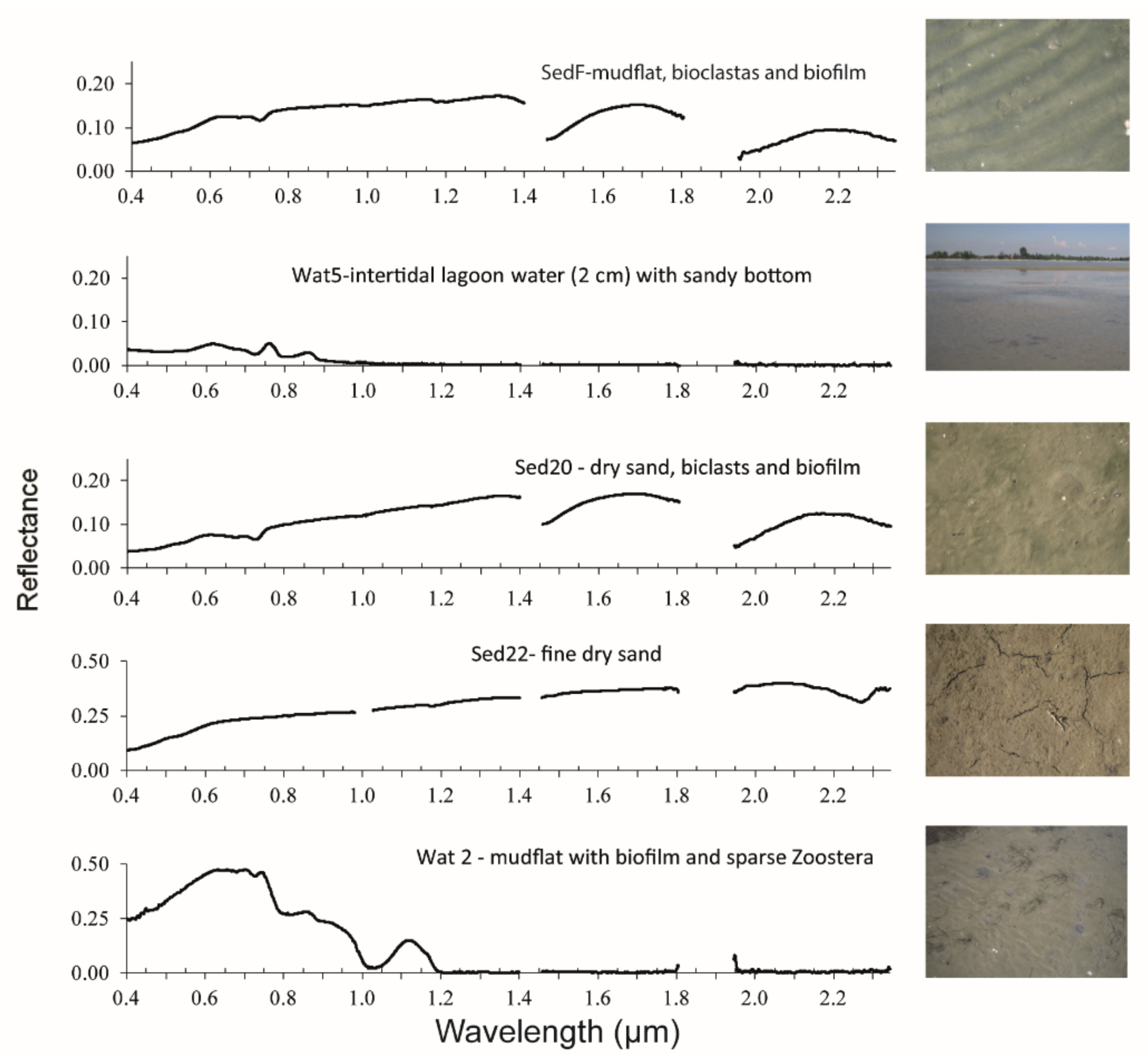
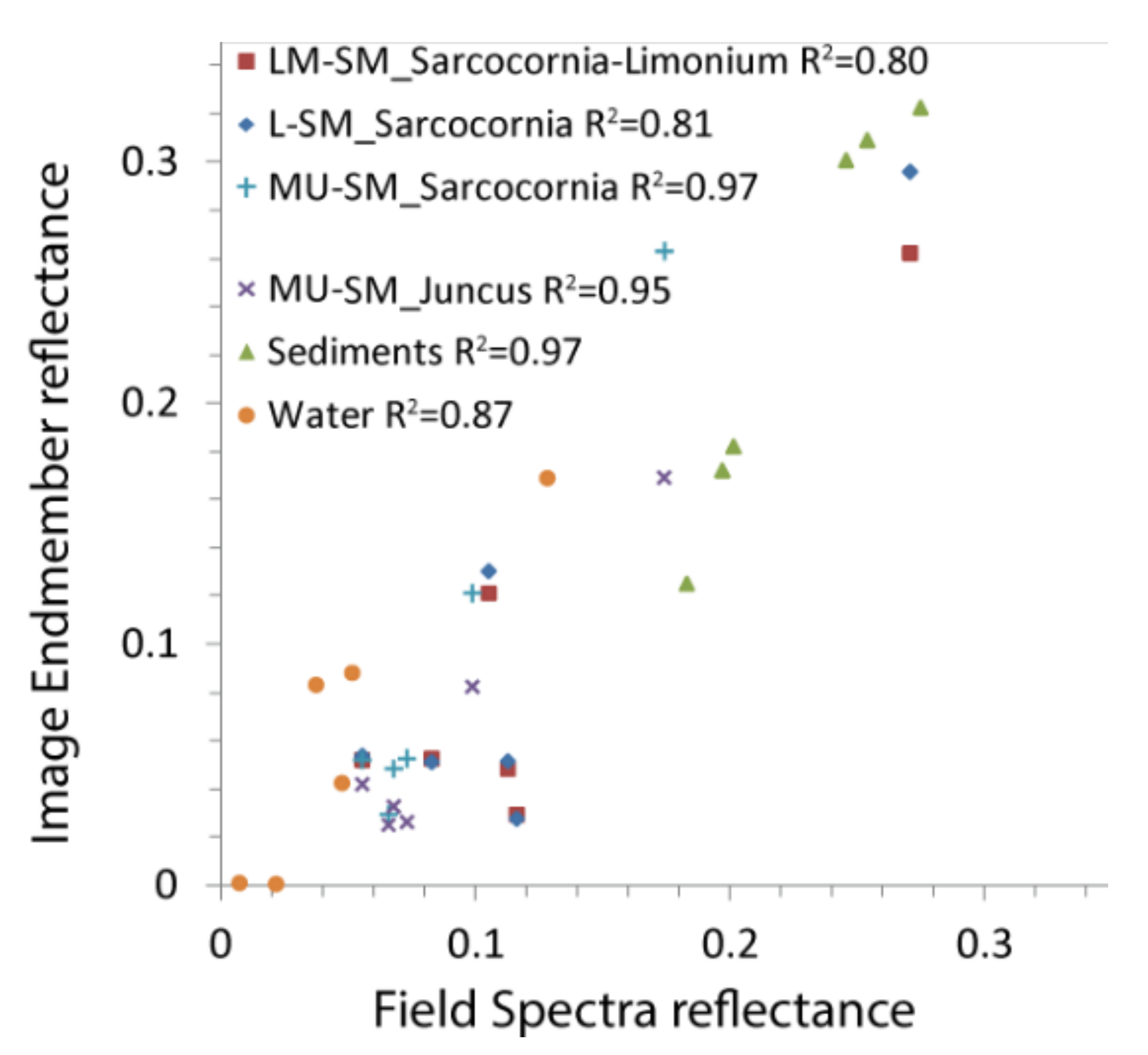
4.1.1. Endmembers’ Validation: The Field Spectral Library

Six endmembers have been distinguished through their spectral signature looking at the axes of the Landsat multi-temporal scatterplot, namely sediment, shallow water, two types of vegetation cover (with low and high reflectance), Algae-Biofilm, and water. The spectral signatures of the endmembers are validated using the field spectral library collected in 2013 (Figure 6).

Vegetation with low reflectance corresponds to the upper saltmarsh and, more specifically, to the transition between Sarcocornia-Limonium and Juncus. On the other hand, vegetation with high reflectance values corresponds to the lower saltmarsh, specifically to Sarcocornia-Limonium and Sarcocornia (Figure 7). The identification of the different vegetation typologies (i.e., Sarcocornia, Limonium, Juncus, and Algae) is possible through the correlation between the pixel spectral signature and the field data. Above 2500 spectral bands were resampled according to the satellite sensor spectral features (i.e., the spectral bands of the sensors on board Landsat-4, Landsat-5, and Landsat-7). This procedure assures the representativeness of the endmembers in the study area. The endmembers’ validation provided well-fitted correlation for both Juncus (R² > 0.90) and Sarcocornia-Limonium (R² > 0.80) (Figure 7).

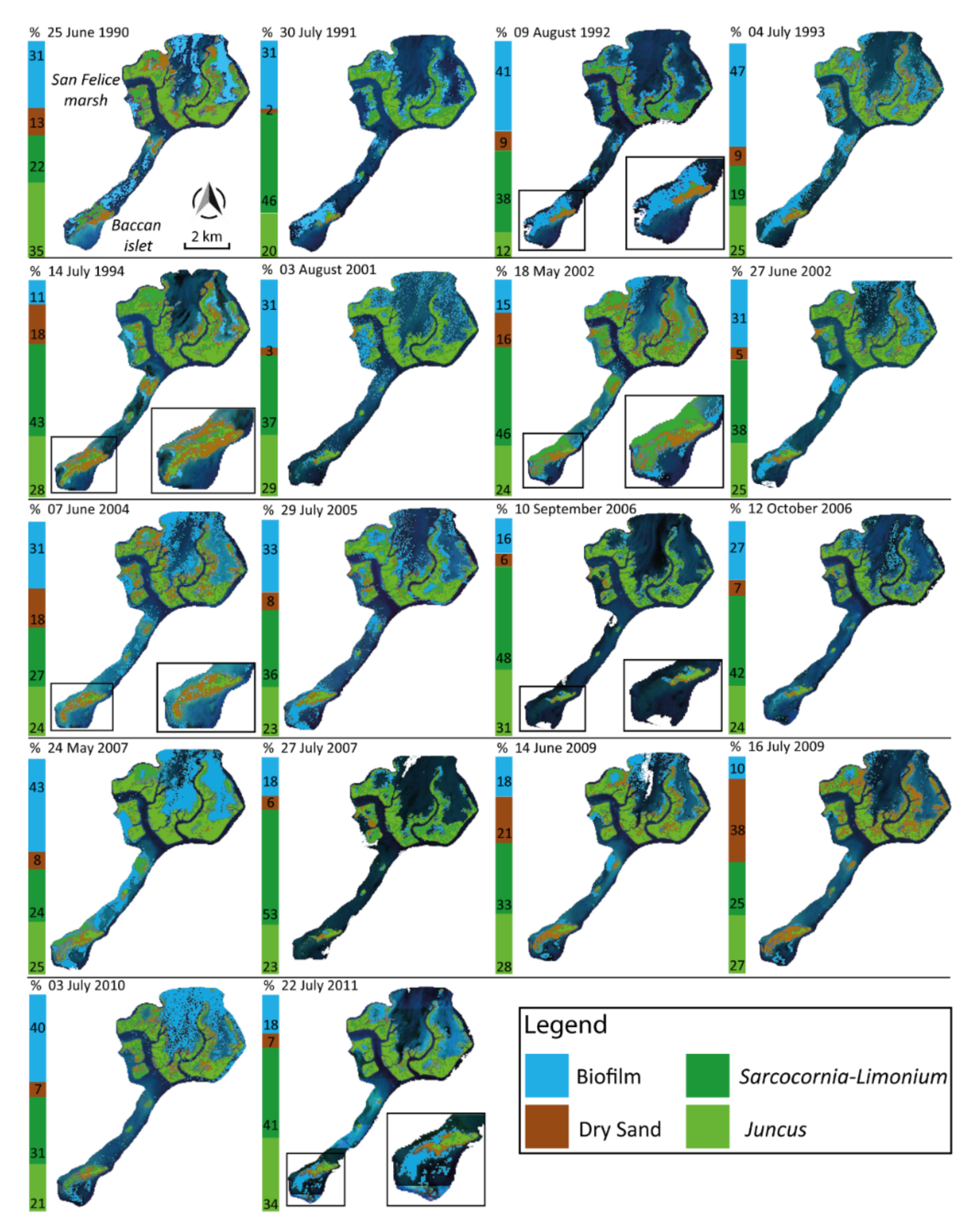
4.1.2. Classification of Spatial Patterns

Once the endmembers are defined and validated through the field spectral library, the LSMA allows for detecting their fractional cover abundance at a pixel level (30 × 30 m). Specifically, the fraction extraction and its yearly distribution in the period covered by the Landsat images (1990 to 2011) has been analyzed for Algae-Biofilm, dry sand, Sarcocornia-Limonium, and Juncus mixture due to their representativeness spatiotemporal variation in the study area (Figure 8). Looking specifically in 1992, 1994, 2002, 2004, 2006, and 2011 in Figure 8, the spatial variation of the cover fractions within the Baccan islet, located in front of Lido Channel, it can be observed: (i) the replacement of Juncus mixture by dry sand in the period of 1994–2004; (ii) the disappearance of dry sand in a large area in the Southern part of the catchment between 2004–2006, and (iii) the presence of Algae-Biofilm in 2011 and 1992.

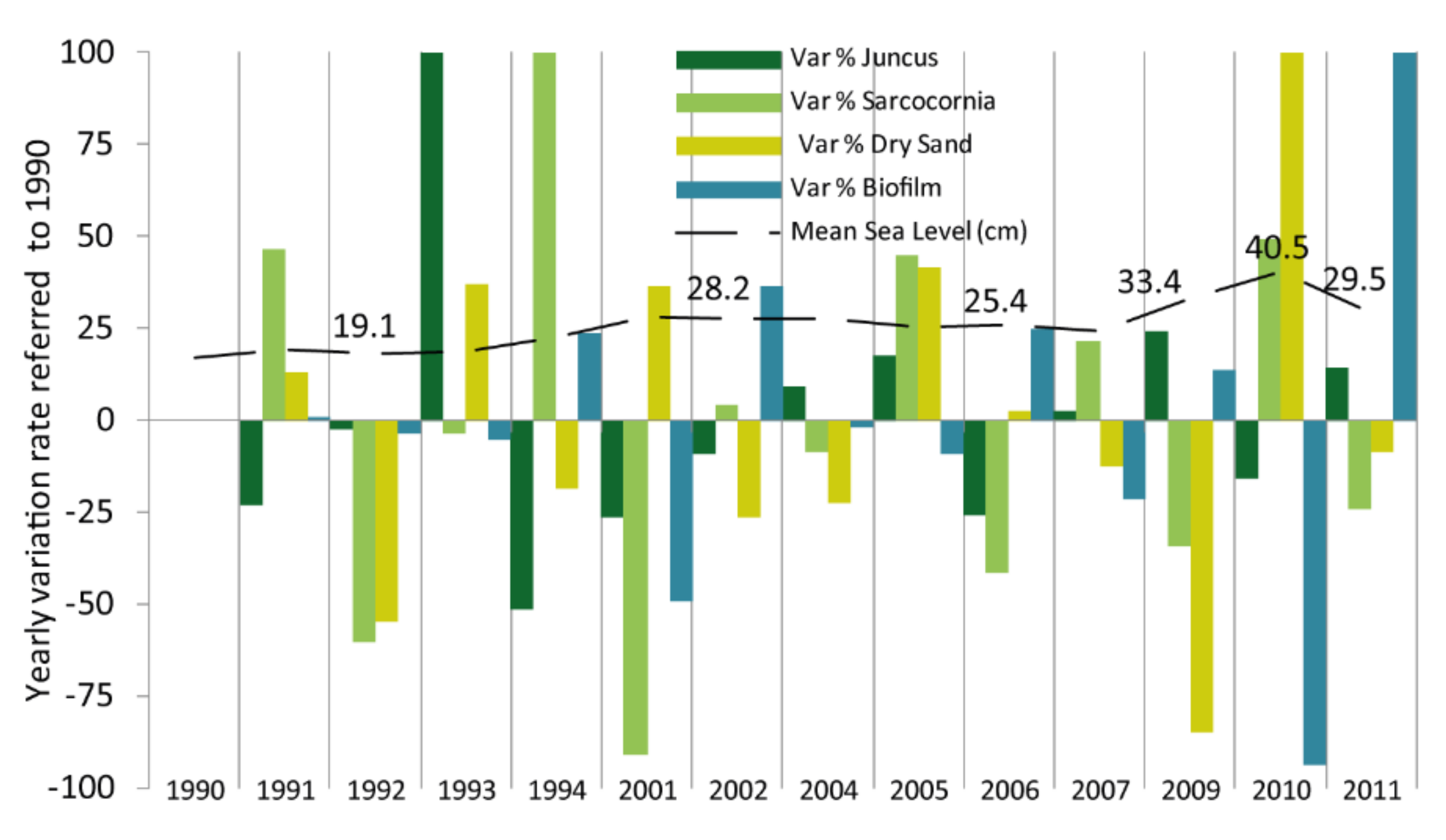
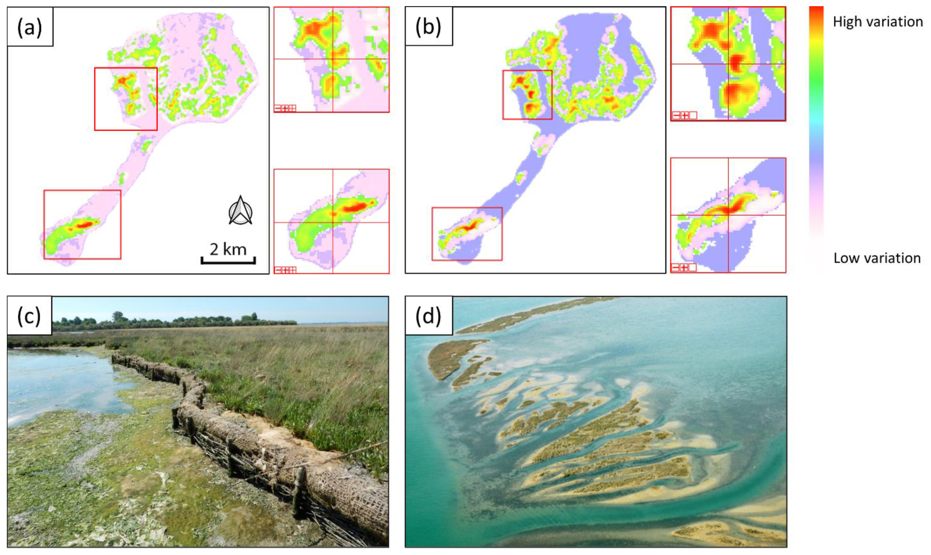
4.1.3. Rate of Variation in the Spatial Patterns’ Distribution

The annual rate of variation in the spatial patterns’ distribution has been quantified for all four cover typologies and compared with the mean sea level. The analysis assesses the amount of change using 1990 as reference year rather than the absolute quantity. A significant reduction of the vegetation distribution is detected after 1994 (Figure 9). This fact could be related to the increased mean sea level (changing from 22.7 cm in 1994 to 28.2 cm in 1995, and with the highest peak in the last decade of 40.5 cm in 2010) (Figure 9), and especially the increased frequency of tide levels over 110 cm (going from 125 in 1994 to 799 in 1995, with the highest peak of 3657 also in 2010) (Figure 3).

4.2. Spatiotemporal Analysis

Based on the vegetation cover typologies previously identified through the satellite image classification, the spatiotemporal trends are analyzed within the Lido basin in the period of 1990–2011. The aim is clearly identifying the areas that are more likely inducible to a critical state. This way, the natural (climatic, hydrodynamic, or morphological) as well as the human-induced variables that influence and intensify this changing behavior can also be identified over the studied period.

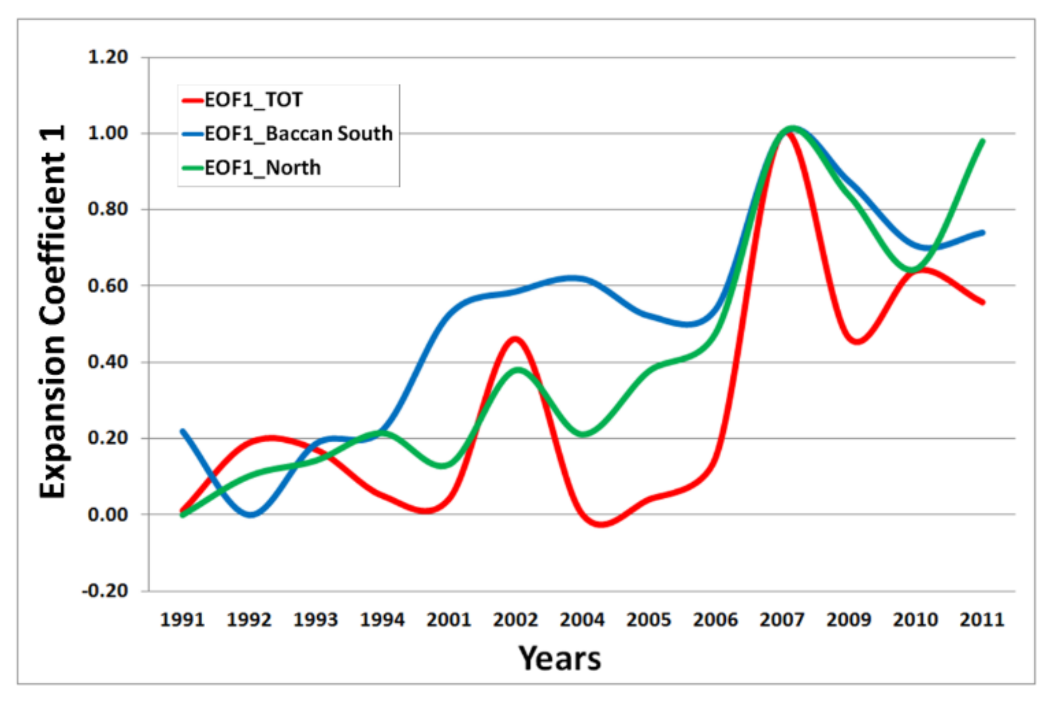
4.2.1. Temporal Trends: The Empirical Orthogonal Function (EOF)

The whole study area shows a trend of growing temporal change as an increase in the EOF expansion coefficients among the studied years. Looking at the total EOF expansion coefficient 1 (EOF 1) for the upper saltmarsh—the stable part of the vegetation cover—the temporal variations are more punctual, with specific peaks in 2001–2004 and 2006–2009 (Figure 10).

These above peaks are frequently natural-(climatic) or human-induced change events. Specially, the maps of EOF expansion coefficient 2 (EOF 2) allow to indicate that changes in the upper saltmarsh and sediment stability are more significant in the Central and Southern part than in the Northern part (Figure 11). EOF 1 shows the most obvious variations (Figure 10). This is the time course of the most typical changes. Instead, EOF 2 allowed detecting the time course of less typical changes either natural or human-induced (Figure 11).

The heterogeneous nature of the investigated site suggests that EOF changes are related to both natural and anthropogenic factors. So, considering the artificial anthropogenic restoration of the Lagoon morphology, the EO data-based pattern analysis shows the spatial and temporal variability, highlighting changes of state over time that have to be interpreted using the PLD.

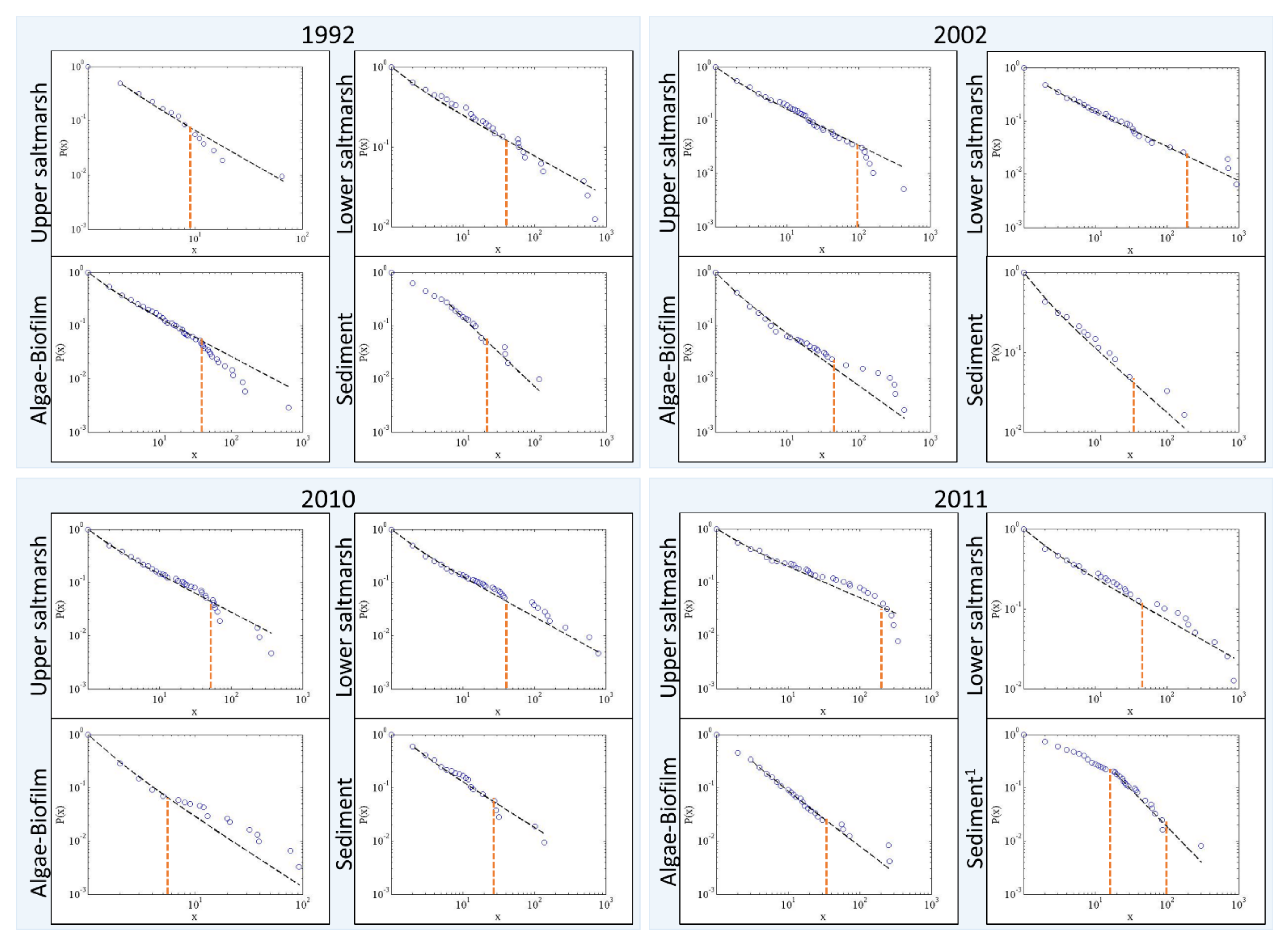
4.2.2. Spatial Trends: The Power Law Distribution (PLD)

Changes from power laws identify stochastic conditions. The PLD allows for analyzing the interaction among the vegetation and sediment patch size. A frequent deviation in the tail of the distributions is related to the larger upper saltmarsh’s patches (Figure 12). Disturbance-recovery processes result in predictable patterns over a range of spatial scale. Despite the patterns’ irregularity, the graph shows that patches of all sizes are characterized by a predictable PLD.

Figure 12 shows the PLD results for the years of higher interest in terms of linearity deviations, namely 1992, 2002, 2010, and 2011. Firstly, 1992 shows an important increase in the frequency of tide levels over 110 cm (Figure 3). The PLD of the lower saltmarsh shows a linear trend, related to more resilient and adaptive species to tide variations (pulsating, seasonal and interannual events). Instead, the upper saltmarsh PLD follows a non-linear trend of the largest patches. This fact can be related to climatic conditions, i.e., frequent tide levels exceeding 110 cm. As for Algae-Biofilm, significant variations occur. This element of the ecosystem increases its spatial expansion as a significant part of the surface subjected to the variation of the tide increases, thereby undergoing a colonization of the diatoms, which begins to build the mudflat and contributes to vertical accretion. Additionally, in 1992, there is a higher frequency of the smaller patches than in previous years. The PLD of the sediment shows a linear trend with little significant variations but the inexistence of large patches.

The period until 2002 is characterized by a constant increasing trend of the mean sea level and a variable frequency of tide levels over 110 cm (Figure 3). The PLD of the lower saltmarsh perfectly follows a linear trend. Instead, the upper saltmarsh shows a significant deviation in its tail for larger patches.

The year 2010 is characterized by an increase in the trend of sea level measurements, as well as a significant increase in the frequency of tide levels over 110 cm (over 2500). The winter periods 2009–2010 and 2008–2009 were characterized by numerous episodes of high tide and heavy rainfall and are anomalous in comparison to the last 30 years. The lower saltmarsh shows its more fragmented part in the Baccan islet. There is no detour. The trend of the PLD in 2010 is like that of the upper saltmarsh in which the frequency size of the patches is linear but some intermediate size classes are missing. Previous years are characterized by a more pronounced variation of the size frequencies. Instead, the period of 2009–2010 undergoes a more gradual variation. As for the Algae-Biofilm, the size frequency distribution follows a linear trend with a deviation towards larger patches. The exposed part is greater, probably due to the decreasing tide level in 2009, and the larger patches are evident. Finally, the sediment PLD shows less frequency of larger patches. This fact is related to the coverage of biofilm. The graph shows the lack of intermediate classes and never reaches large patches.

2011 is the last studied year of the time series. It is significant because of the sea and tide levels. The lower saltmarsh shows linearity on its PLD trend and a higher frequency of larger sizes. The distribution of patch sizes is gradual and well distributed with a greater density of the intermediate classes. As for the upper saltmarsh, the PLD shows a high deviation for larger patches. The Algae-Biofilm has a similar trend to the lower saltmarsh.

As for the sediment, the PLD of 2004 is clearly related to the changes displayed by the EOF (Figure 10, year 2004). The sediment PLD greatly increases the slope and the absence of larger patches highlights an unstable phase (Figure 12, bottom right).

5. Discussion

The analysis and implemented conceptual models allow evaluating spatial patterns (i.e., small to large patches) and the time range within these patterns fluctuate before a change of state. The analysis of threshold values makes it also possible to understand the stability of these systems with respect to disturbances and risks associated with climate change or anthropogenic alterations.

Open satellite data analysis, namely the LSMA, the EOF, and the PLD have been used to spatiotemporally characterize the saltmarsh in the Lido basin in the Venice Lagoon. The LSMA allows obtaining a preliminary classification of the entire study area with the extrapolation of vegetation, sediment, and biofilm cover typologies, while the EOF characterizes vegetation and sediment interannual trends.

The observed peaks in the EOF maps and the deviation in the tails of the PLD, specifically in the period of 2001–2004 and 2006–2009, allowed detecting the main changes in the system.

Specifically, in the EOF results (Figure 10 and Figure 11), it is possible to see the effect of artificial mudflats reconstruction, protected by wooden piles along their perimeter (Figure 11c). Jetties, confined disposal facilities, dredging operations, and mobile barriers on the sea-bottom were carried out together with morphological restoration of intertidal areas in the mentioned years.

The PLD deviation points out changes in environmental conditions at saltmarsh edge (Figure 12). The deviation in the tail of the distributions related to the largest patches (the more resistant in terms of stability) is observed in the periods of major variance in tidal levels’ frequency and this represents a critical state change influenced by hydrodynamics of the area.

The upper saltmarsh shows linearity along the temporal series, even with the inexistence of the major patch classes, i.e., there is no change in the slope but a minimal deviation of the tail. As for the Algae-Biofilm, the PLD of 2002 shows the deviation of the tail towards the larger patches. Conversely, in the same and in the following years, the sediment shows a linear distribution, never reaching the largest patches. This fact could explain an extension of the stable mudflat surface. In 2004, the sediment shows an increase of the intermediate classes whereas almost an absence of the larger ones and a double slope in the trend line. Small patches are gradually progressing until the intermediate sizes. The decrease in the tide level can be associated to the larger percentage of sediment presence (18%).

The only strongly aggregated point is found in the Baccan area that is located in front of the Lido inlet and thereby more sensitive to the changes in the hydrodynamic regime. The results suggest that a feedback mechanism, mediated by microphytobenthos’ influence, causes sediment bio-stabilization. This may explain the exceptional preservation of the intertidal mudflats in the Northern part of the study area [19,72,85]. Such a mechanism [18,19] can be detected by the EO methods for the three steps as follows (Figure 13):

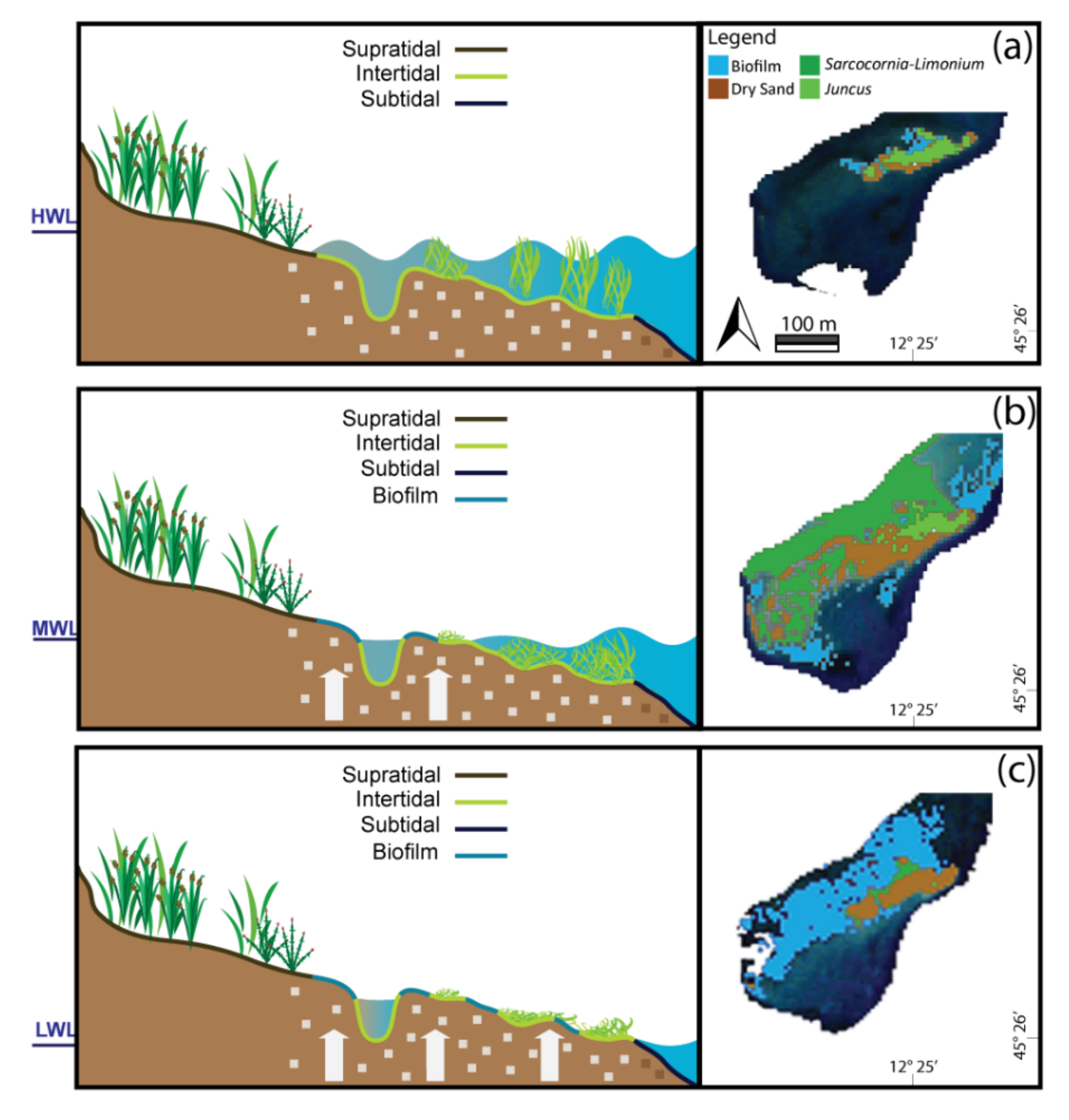
• Step A: Subtidal areas, which are colonized by seagrass, are better protected against erosion compared to unvegetated areas. The ability of vegetation to reduce the applied bed shear stress enhances deposition of suspended sediment.
• Step B: Vertical accretion can occur over time; bottom sediments are elevated from a subtidal to an intertidal environment, where time of exposure is higher.
• Step C: Micro-organisms (diatoms and cyanobacteria), which are more abundant in intertidal environments, start colonizing the substrata producing Extracellular Polymeric Substances (EPS), particularly during summer and intertidal exposure, and increasing the erosion threshold and sediment stability (i.e., resistance against sediment waves and tidal currents).

This feedback mechanism can be correlated to human interventions at the main three inlets of Venice Lagoon, where the construction of jetties was necessary for the placement of MOSE’s barriers on the seafloor. In the last 30 years, morphological structures were realized with the reuse of about 19.5 × 106 m³ of sediments from dredging channels. At the beginning-early 1990s, re-implantation of sea grass (Zoostera marina on sandy subtidal areas and Zoostera noolti) was tested because vegetation cover favors siltation and morphological restoration of shoals and intertidal flats. Then, dredging of sediments from navigation channels and their use to increase the elevation of velme (mudflat) and barene (saltmarshes) was the most common approach since 2000.

It does not surprise that in the period of 1989–2015, the presence of ornithic species has been targeted to understand how the artificial barren islands were populated. For example, for the little tern, even considering the natural fluctuating behavior of the species in the Lagoon during the nesting periods, a preference for the artificial barrens has been recorded with a complete abandonment of the natural barrens [86].

Considering the feedback mechanism proposed by [19], which explains how micro-organisms contribute to the seasonal stabilization of sediments in the Northern intertidal mudflats of the Venice Lagoon, the change of state highlighted in the PLD results could imply a passage from one ecosystem regime to another, and therefore between basins of attraction—or stable states. The environment can take on different states driven by external changes that lead to the transition from one to another. The system opposes these changes until it reaches a threshold value, the deviation from linearity, specifically in 1992, 2002, 2010, and 2011, where internal relations begin to break. It is in fact maintained by internal relations between species, but at the same time, these dynamics can interact with forcing that act on larger scales.

Therefore, the saltmarsh vegetation patterns, as well as their irregular spatial structure and its self-organization, could be used as an indicator of the ecosystem stability, either inducing steady states or pushing the ecosystem towards transition state dynamics [27,51,72,85]. The spatiotemporal trends can show the modulation of the system response to external drivers over time and support the estimation of the system resistance or resilience stability to disturbances. There is evidence of different inclinations of the PLD as well as different degrees of deviations over vegetation typologies and sediment over time. Detecting and understanding these trends is important to contribute to the description and forecasting of wetland ecosystems.

It could also be considered how the method can be applied to the MOSE management for the bio-stabilization processes during prolonged periods of still-water condition within the Lagoon. Will the closure of the mobile barriers influence the sedimentation and sediment stabilization processes and the morphological changes?

Effects of global change on development and sustainability of Venice Lagoon management is taken in great consideration. In 2012, CVN investigated the possibility to use the MOSE not only to protect the city of Venice from Acqua Alta, but also to partially open the floodgates in order to exploit nature-based energy (tidal cycles) to force or slow down flows within the Lagoon by using and generating different water level between the Northern and Southern part.

Changes in tidal height and frequency or the reclamation of lands over the intertidal zones can create unpredictable environments where there may be changes in bio-geophysical variables. Studies regarding the adaptation of water level changes and the response of ecosystem structure (i.e., the biological communities) and functions (i.e., the state transition from bare tidal flat to saltmarshes) are widely developed, i.e., the Eastern Asian coastal ecoregion [61]. Key threatening processes often include damming and sea level rise or modification of the large systems inducing degradation, fragmentation and decline in the areal extent of tidal flats, which can lead to increased risk for the biodiversity [87], making available interesting analogies with the uniqueness of the MOSE effects in the Venice Lagoon unless the spatial scales and the climate region.

With this study, we are aiming at observing and discussing the bridge between the short-term (decadal) and long-term (3 decades) ecosystem-level transitions driven by the summed effects of sea level and human-driven changes of the Lagoon hydraulics. It is a contribution to studies on the adaptive capacities of biological communities and it contributes to better understanding of ecosystem state transitions.

Findings of the present paper can support coastal wetlands restoration programs that aim to increase the resilience of systems considering different scenarios of sea level rise and the natural capital conservation (i.e., the value of being a Ramsar and a Natura 2000 site). The system of adaptive management enables adjustments to be made at a site level but also touching the regional level, particularly in response to the impacts of natural- or human-driven events affecting water-sediment-vegetation patterns. It is important to highlight that adaptation initiatives need to be analyzed on both short- and long-term and both wide to fine scale.

Sustainable management and conservation agendas commonly include the requirements for mapping and monitoring environmental patterns and processes because, without monitoring and data collection, stakeholders are unable to implement conservation and short- and long-term protection actions, which are the fundamentals for planning anthropogenic activities, risk recovery, and prevention actions [88].

6. Conclusions

The present manuscript presents an approach, mainly based on satellite imagery acquired from Landsat, that allows identifying ecosystem-level indicators, and assessing the state transition dynamics in the Lido basin in the North of Venice Lagoon (North-East of Italy) in the period of 1990–2011. The methodology is based on multi-temporal and spatial EO-based analysis (the EOF and the PLD), thereby allowing its application elsewhere. The results of the spatial pattern analysis (PLD) manifest the influence of external drivers, mainly derived by anthropogenic activities. PLD’s thresholds prove to be an effective method to detect changes in the size frequency distribution of different cover classes (upper and lower saltmarsh, Algae-Biofilm and sediment). Finally, the work has derived a conceptual model on bio-stabilization processes linked to morphological restoration.

The studied wetland can be considered an example of what is happening in many other wetlands due to sea level rise effects or hydrodynamic regime due to management. The EO-based analysis, coupled with climate data, measures of changes in erosion patterns, and water quality, can make different areas comparable. Moreover, biologically, short- and long-term repetition of environmental parameters’ change have great impact on the aquatic species’ adaptability. Therefore, the current approach can be further developed monitoring the response and resilience of environment to climate changes and/or human impacts on fishes and other species, the sediment transport and water quality (i.e., Anthropocene evidence). This would allow continuing the improvement of the understanding of the ecological response, scaling up from ecosystem-level to landscape-level indicators.

Considering the development of the current use of Copernicus data and products, and the European Commission’s six high-priority candidate missions to address EU’s policies and gaps in Copernicus users’ needs, the presented operational method, tested on Landsat data, could be further expanded. Specifically, considering within the six upcoming missions the analysis of data from CHIME (Copernicus Hyperspectral Imaging Mission), the method applied in this study will optimize, as a monitoring tool, the set of results already analyzed in this context.

References

1. Church, M.; Dudill, A.; Venditti, J.G.; Frey, P. Are Results in Geomorphology Reproducible? J. Geophys. Res. Earth Surf. 2020, 125. [Google Scholar] [CrossRef]
2. Dietrich, W.E.; Perron, J.T. The search for a topographic signature of life. Nature 2006, 439, 411–418. [Google Scholar] [CrossRef]
3. Kirwan, M.L.; Murray, A.B. Tidal marshes as disequilibrium landscapes? Lags between morphology and Holocene sea level change. Geophys. Res. Lett. 2008, 35, L24401. [Google Scholar] [CrossRef]
4. Kirwan, M.L.; Murray, A.B. Ecological and morphological response of brackish tidal marshland to the next century of sea level rise: Westham Island, British Columbia. Glob. Planet. Chang. 2008, 60, 471–486. [Google Scholar] [CrossRef]
5. Corenblit, D.; Steiger, J. Vegetation as a major conductor of geomorphic changes on the Earth surface: Toward evolutionary geomorphology. Earth Surf. Process. Landf. 2009, 34, 891–896. [Google Scholar] [CrossRef]
6. Reinhardt, L.; Jerolmack, D.; Cardinale, B.J.; Vanacker, V.; Wright, J. Dynamic interactions of life and its landscape: Feedbacks at the interface of geomorphology and ecology. Earth Surf. Process. Landf. 2010, 35, 78–101. [Google Scholar] [CrossRef]
7. Zhang, X.; Fichot, C.G.; Baracco, C.; Guo, R.; Neugebauer, S.; Bengtsson, Z.; Ganju, N.; Fagherazzi, S. Determining the drivers of suspended sediment dynamics in tidal marsh-influenced estuaries using high-resolution ocean color remote sensing. Remote Sens. Environ. 2020, 240, 111682. [Google Scholar] [CrossRef]
8. Marani, M.; Belluco, E.; Ferrari, S.; Silvestri, S.; D’Alpaos, A.; Lanzoni, S.; Feola, A.; Rinaldo, A. Analysis, synthesis and modelling of high-resolution observations of salt-marsh eco-geomorphological patterns in the Venice lagoon. Estuar. Coast. Shelf Sci. 2006, 69, 414–426. [Google Scholar] [CrossRef]
9. Carr, J.A.; D’Odorico, P.; McGlathery, K.J.; Wiberg, P.L. Modeling the effects of climate change on eelgrass stability and resilience: Future scenarios and leading indicators of collapse. Mar. Ecol. Prog. Ser. 2012, 448, 289–301. [Google Scholar] [CrossRef] [Green Version]
10. Carr, J.A.; D’Odorico, P.; McGlathery, K.J.; Wiberg, P.L. Stability and resilience of seagrass meadows to seasonal and interannual dynamics and environmental stress. J. Geophys. Res. Biogeosci. 2012, 117. [Google Scholar] [CrossRef]
11. Fagherazzi, S.; Kirwan, M.L.; Mudd, S.M.; Guntenspergen, G.R.; Temmerman, S.; D’Alpaos, A.; Van De Koppel, J.; Rybczyk, J.M.; Reyes, E.; Craft, C.; et al. Numerical models of salt marsh evolution: Ecological, geomorphic, and climatic factors. Rev. Geophys. 2012, 50. [Google Scholar] [CrossRef]
12. Mariotti, G.; Fagherazzi, S. A numerical model for the coupled long-term evolution of salt marshes and tidal flats. J. Geophys. Res. Earth Surf. 2010, 115. [Google Scholar] [CrossRef]
13. Taramelli, A.; Valentini, E.; Cornacchia, L. Remote sensing solutions to monitor biotic and abiotic dynamics in coastal ecosystems. In Coastal Zones: Solutions for the 21st Century; Elsevier Inc.: Amsterdam, The Netherlands, 2015; pp. 125–138. ISBN 9780128027592. [Google Scholar]
14. Murray, A.B.; Lazarus, E.; Ashton, A.; Baas, A.; Coco, G.; Coulthard, T.; Fonstad, M.; Haff, P.; McNamara, D.; Paola, C.; et al. Geomorphology, complexity, and the emerging science of the Earth’s surface. Geomorphology 2009, 103, 496–505. [Google Scholar] [CrossRef]
15. Black, K.S.; Paterson, D.M. LISP-UK Littoral Investigation of Sediment Properties: An introduction. Geol. Soc. Spec. Publ. 1998, 139, 1–10. [Google Scholar] [CrossRef]
16. Conley, D.J. Biogeochemical nutrient cycles and nutrient management strategies. Hydrobiologia 1999, 410, 87–96. [Google Scholar] [CrossRef]
17. Wang, C.; Schepers, L.; Kirwan, M.L.; Belluco, E.; D’Alpaos, A.; Wang, Q.; Yin, S.; Temmerman, S. Different coastal marsh sites reflect similar topographic conditions for bare patches and vegetation recovery. Earth Surf. Dyn. Discuss. 2021, 9, 71–88. [Google Scholar] [CrossRef]
18. Amos, C.L.; Bergamasco, A.; Umgiesser, G.; Cappucci, S.; Cloutier, D.; Denat, L.; Flindt, M.; Bonardi, M.; Cristante, S. The stability of tidal flats in Venice Lagoon—The results of in-situ measurements using two benthic, annular flumes. J. Mar. Syst. 2004, 51, 211–241. [Google Scholar] [CrossRef]
19. Cappucci, S.; Amos, C.L.; Hosoe, T.; Umgiesser, G. SLIM: A numerical model to evaluate the factors controlling the evolution of intertidal mudflats in Venice Lagoon, Italy. J. Mar. Syst. 2004, 51, 257–280. [Google Scholar] [CrossRef]
20. Dyer, K.R. The typology of intertidal mudflats. Geol. Soc. Spec. Publ. 1998, 139, 11–24. [Google Scholar] [CrossRef]
21. Dyer, K.R.; Christie, M.C.; Feates, N.; Fennessy, M.J.; Pejrup, M.; Van Der Lee, W. An investigation into processes influencing the morphodynamics of an intertidal mudflat, the Dollard Estuary, the Netherlands: I. Hydrodynamics and suspended sediment. Estuar. Coast. Shelf Sci. 2000, 50, 607–625. [Google Scholar] [CrossRef]
22. Wang, C.; Temmerman, S. Does biogeomorphic feedback lead to abrupt shifts between alternative landscape states?: An empirical study on intertidal flats and marshes. J. Geophys. Res. Earth Surf. 2013, 118, 229–240. [Google Scholar] [CrossRef] [Green Version]
23. Adam, P. Saltmarsh Ecology; Cambridge University Press: Cambridge, MA, USA, 1990; ISBN 9780521245081. [Google Scholar]
24. Vandenbruwaene, W.; Temmerman, S.; Bouma, T.J.; Klaassen, P.C.; De Vries, M.B.; Callaghan, D.P.; Van Steeg, P.; Dekker, F.; Van Duren, L.A.; Martini, E.; et al. Flow interaction with dynamic vegetation patches: Implications for biogeomorphic evolution of a tidal landscape. J. Geophys. Res. Earth Surf. 2011, 116. [Google Scholar] [CrossRef] [Green Version]
25. Weerman, E.J.; Van Belzen, J.; Rietkerk, M.; Temmerman, S.; Kéfi, S.; Herman, P.M.J.; Van De Koppel, J. Changes in diatom patch-size distribution and degradation in a spatially self-organized intertidal mudflat ecosystem. Ecology 2012, 93, 608–618. [Google Scholar] [CrossRef] [Green Version]
26. Taramelli, A.; Valentini, E.; Cornacchia, L.; Mandrone, S.; Monbaliu, J.; Hoggart, S.P.G.; Thompson, R.C.; Zanuttigh, B. Modeling uncertainty in estuarine system by means of combined approach of optical and radar remote sensing. Coast. Eng. 2014, 87, 77–96. [Google Scholar] [CrossRef]
27. Taramelli, A.; Valentini, E.; Cornacchia, L.; Monbaliu, J.; Sabbe, K. Indications of Dynamic Effects on Scaling Relationships Between Channel Sinuosity and Vegetation Patch Size Across a Salt Marsh Platform. J. Geophys. Res. Earth Surf. 2018, 123, 2714–2731. [Google Scholar] [CrossRef]
28. Taramelli, A.; Valentini, E.; Cornacchia, L.; Bozzeda, F. A Hybrid Power Law Approach for Spatial and Temporal Pattern Analysis of Salt Marsh Evolution. J. Coast. Res. 2017, 77, 62–72. [Google Scholar] [CrossRef] [Green Version]
29. Rietkerk, M.; van de Koppel, J. Regular pattern formation in real ecosystems. Trends Ecol. Evol. 2008, 23, 169–175. [Google Scholar] [CrossRef]
30. Zhao, L.-X.; Xu, C.; Ge, Z.-M.; van de Koppel, J.; Liu, Q.-X. The shaping role of self-organization: Linking vegetation patterning, plant traits and ecosystem functioning. Proc. R. Soc. B Biol. Sci. 2019, 286, 20182859. [Google Scholar] [CrossRef] [PubMed]
31. Pascual, M.; Guichard, F. Criticality and disturbance in spatial ecological systems. Trends Ecol. Evol. 2005, 20, 88–95. [Google Scholar] [CrossRef] [PubMed]
32. Scheffer, M.; Bascompte, J.; Brock, W.A.; Brovkin, V.; Carpenter, S.R.; Dakos, V.; Held, H.; Van Nes, E.H.; Rietkerk, M.; Sugihara, G. Early-warning signals for critical transitions. Nature 2009, 461, 53–59. [Google Scholar] [CrossRef]
33. Reed, J.; Shannon, L.; Velez, L.; Akoglu, E.; Bundy, A.; Coll, M.; Fu, C.; Fulton, E.A.; Grüss, A.; Halouani, G.; et al. Ecosystem indicators—Accounting for variability in species’ trophic levels. ICES J. Mar. Sci. 2017, 74, 158–169. [Google Scholar] [CrossRef]
34. Solé, R.V.; Ferrer-Cancho, R.; Montoya, J.M.; Valverde, S. Selection, tinkering, and emergence in complex networks. Complexity 2002, 8, 20–33. [Google Scholar] [CrossRef]
35. Van de Koppel, J.; van der Wal, D.; Bakker, J.P.; Herman, P.M.J. Self-organization and vegetation collapse in salt marsh ecosystems. Am. Nat. 2005, 165. [Google Scholar] [CrossRef] [Green Version]
36. Kéfi, S.; Rietkerk, M.; Alados, C.L.; Pueyo, Y.; Papanastasis, V.P.; ElAich, A.; De Ruiter, P.C. Spatial vegetation patterns and imminent desertification in Mediterranean arid ecosystems. Nature 2007, 449, 213–217. [Google Scholar] [CrossRef]
37. Friend, P.L.; Ciavola, P.; Cappucci, S.; Santos, R. Bio-dependent bed parameters as a proxy tool for sediment stability in mixed habitat intertidal areas. Cont. Shelf Res. 2003, 23, 1899–1917. [Google Scholar] [CrossRef]
38. Solé, R.V.; Manrubia, S.C.; Benton, M.; Kauffman, S.; Per, B. Criticality and scaling in evolutionary ecology. Trends Ecol. Evol. 1999, 14, 156–160. [Google Scholar] [CrossRef]
39. Malamud-Roam, F.; Lynn Ingram, B. Late Holocene δ13C and pollen records of paleosalinity from tidal marshes in the San Francisco Bay estuary, California. Quat. Res. 2004, 62, 134–145. [Google Scholar] [CrossRef]
40. Schoelynck, J.; de Groote, T.; Bal, K.; Vandenbruwaene, W.; Meire, P.; Temmerman, S. Self-organised patchiness and scale-dependent bio-geomorphic feedbacks in aquatic river vegetation. Ecography 2012, 35, 760–768. [Google Scholar] [CrossRef]
41. Small, C.; Sousa, D. Humans on Earth: Global extents of anthropogenic land cover from remote sensing. Anthropocene 2016, 14, 1–33. [Google Scholar] [CrossRef] [Green Version]
42. Fagherazzi, S.; Mariotti, G.; Leonardi, N.; Canestrelli, A.; Nardin, W.; Kearney, W.S. Salt Marsh Dynamics in a Period of Accelerated Sea Level Rise. J. Geophys. Res. Earth Surf. 2020, 125. [Google Scholar] [CrossRef]
43. Donatelli, C.; Zhang, X.; Ganju, N.K.; Aretxabaleta, A.L.; Fagherazzi, S.; Leonardi, N. A nonlinear relationship between marsh size and sediment trapping capacity compromises salt marshes’ stability. Geology 2020, 48, 966–970. [Google Scholar] [CrossRef]
44. Antonioli, F.; Anzidei, M.; Amorosi, A.; Lo Presti, V.; Mastronuzzi, G.; Deiana, G.; De Falco, G.; Fontana, A.; Fontolan, G.; Lisco, S.; et al. Sea-level rise and potential drowning of the Italian coastal plains: Flooding risk scenarios for 2100. Quat. Sci. Rev. 2017, 158, 29–43. [Google Scholar] [CrossRef] [Green Version]
45. Scheffer, M.; Carpenter, S.; Foley, J.A.; Folke, C.; Walker, B. Catastrophic shifts in ecosystems. Nature 2001, 413, 591–596. [Google Scholar] [CrossRef]
46. Falcieri, F.M.; Benetazzo, A.; Sclavo, M.; Russo, A.; Carniel, S. Po River plume pattern variability investigated from model data. Cont. Shelf Res. 2014, 87, 84–95. [Google Scholar] [CrossRef]
47. Marani, M.; Lanzoni, S.; Silvestri, S.; Rinaldo, A. Tidal landforms, patterns of halophytic vegetation and the fate of the lagoon of Venice. J. Mar. Syst. 2004, 51, 191–210. [Google Scholar] [CrossRef]
48. Manzo, C.; Valentini, E.; Taramelli, A.; Filipponi, F.; Disperati, L. Spectral characterization of coastal sediments using Field Spectral Libraries, Airborne Hyperspectral Images and Topographic LiDAR Data (FHyL). Int. J. Appl. Earth Obs. Geoinf. 2015, 36, 54–68. [Google Scholar] [CrossRef]
49. Taramelli, A.; Melelli, L. Map of deep seated gravitational slope deformations susceptibility in central Italy derived from SRTM DEM and spectral mixing analysis of the Landsat ETM + data. Int. J. Remote Sens. 2009, 30, 357–387. [Google Scholar] [CrossRef]
50. Valentini, E.; Taramelli, A.; Filipponi, F.; Giulio, S. An effective procedure for EUNIS and Natura 2000 habitat type mapping in estuarine ecosystems integrating ecological knowledge and remote sensing analysis. Ocean Coast. Manag. 2015, 108, 52–64. [Google Scholar] [CrossRef]
51. Finotello, A.; D’Alpaos, A.; Bogoni, M.; Ghinassi, M.; Lanzoni, S. Remotely-sensed planform morphologies reveal fluvial and tidal nature of meandering channels. Sci. Rep. 2020, 10, 1–13. [Google Scholar] [CrossRef]
52. Piedelobo, L.; Taramelli, A.; Schiavon, E.; Valentini, E.; Molina, J.-L.; Nguyen Xuan, A.; González-Aguilera, D. Assessment of Green Infrastructure in Riparian Zones Using Copernicus Programme. Remote Sens. 2019, 11, 2967. [Google Scholar] [CrossRef] [Green Version]
53. Valentini, E.; Taramelli, A.; Cappucci, S.; Filipponi, F.; Xuan, A.N. Exploring the dunes: The correlations between vegetation cover pattern and morphology for sediment retention assessment using airborne multisensor acquisition. Remote Sens. 2020, 12, 1229. [Google Scholar] [CrossRef] [Green Version]
54. Taramelli, A.; Valentini, E.; Righini, M.; Filipponi, F.; Geraldini, S.; Nguyen Xuan, A. Assessing Po River Deltaic Vulnerability Using Earth Observation and a Bayesian Belief Network Model. Water 2020, 12, 2830. [Google Scholar] [CrossRef]
55. Taramelli, A.; Manzo, C.; Valentini, E.; Cornacchia, L. Coastal subsidence: Causes, mapping, and monitoring. In Natural Hazards: Earthquakes, Volcanoes, and Landslides; Singh, R.P., Bartlett, D., Eds.; CRC Press, Taylor & Francis: Boca Raton, FL, USA; Abingdon, UK, 2018; pp. 253–290. ISBN 9781315166841. [Google Scholar]
56. Laengner, M.L.; Siteur, K.; van der Wal, D. Trends in the Seaward Extent of Saltmarshes across Europe from Long-Term Satellite Data. Remote Sens. 2019, 11, 1653. [Google Scholar] [CrossRef] [Green Version]
57. Cappucci, S.; Valentini, E.; Del Monte, M.; Paci, M.; Filipponi, F.; Taramelli, A. Detection of Natural and Anthropic Features on Small Islands. J. Coast. Res. 2017, 2017, 73–87. [Google Scholar] [CrossRef]
58. Taramelli, A.; Lissoni, M.; Piedelobo, L.; Schiavon, E.; Valentini, E.; Xuan, A.N.; González-Aguilera, D. Monitoring green infrastructure for naturalwater retention using copernicus global land products. Remote Sens. 2019, 11, 1583. [Google Scholar] [CrossRef] [Green Version]
59. Bender, D.J.; Contreras, T.A.; Fahrig, L. Habitat loss and population decline: A meta-analysis of the patch size effect. Ecology 1998, 79, 517–533. [Google Scholar] [CrossRef]
60. Jang, J.D.; Chun, S.G.; Kim, K.C.; Jeong, K.Y.; Kim, D.K.; Kim, J.Y.; Joo, G.J.; Jeong, K.S. Long-term adaptations of a migratory bird (Little Tern Sternula albifrons) to quasi-natural flooding disturbance. Ecol. Inform. 2015, 29, 166–173. [Google Scholar] [CrossRef]
61. Murray, N.J.; Ma, Z.; Fuller, R.A. Tidal flats of the Yellow Sea: A review of ecosystem status and anthropogenic threats. Austral. Ecol. 2015, 40, 472–481. [Google Scholar] [CrossRef]
62. Craft, C.; Clough, J.; Ehman, J.; Joye, S.; Park, R.; Pennings, S.; Guo, H.; Machmuller, M. Forecasting the effects of accelerated sea-level rise on tidal marsh ecosystem services. Front. Ecol. Environ. 2009, 7, 73–78. [Google Scholar] [CrossRef] [Green Version]
63. Bonometto, A.; Feola, A.; Rampazzo, F.; Gion, C.; Berto, D.; Ponis, E.; Boscolo Brusà, R. Factors controlling sediment and nutrient fluxes in a small microtidal salt marsh within the Venice Lagoon. Sci. Total Environ. 2019, 650, 1832–1845. [Google Scholar] [CrossRef] [PubMed]
64. Ferla, M.; Cordella, M.; Michielli, L.; Rusconi, A. Long-term variations on sea level and tidal regime in the lagoon of Venice. Estuar. Coast. Shelf Sci. 2007, 75, 214–222. [Google Scholar] [CrossRef]
65. Bettinetti, A.; Pypaert, P.; Sweerts, J.P. Application of an integrated management approach to the restoration project of the lagoon of Venice. J. Environ. Manag. 1996, 46, 207–227. [Google Scholar] [CrossRef]
66. Sarretta, A.; Pillon, S.; Molinaroli, E.; Guerzoni, S.; Fontolan, G. Sediment budget in the Lagoon of Venice, Italy. Cont. Shelf Res. 2010, 30, 934–949. [Google Scholar] [CrossRef] [Green Version]
67. Janowski, L.; Madricardo, F.; Fogarin, S.; Kruss, A.; Molinaroli, E.; Kubowicz-Grajewska, A.; Tegowski, J. Spatial and Temporal Changes of Tidal Inlet Using Object-Based Image Analysis of Multibeam Echosounder Measurements: A Case from the Lagoon of Venice, Italy. Remote Sens. 2020, 12, 2117. [Google Scholar] [CrossRef]
68. Villatoro, M.M.; Amos, C.L.; Umgiesser, G.; Ferrarin, C.; Zaggia, L.; Thompson, C.E.L.; Are, D. Sand transport measurements in Chioggia inlet, Venice lagoon: Theory versus observations. Cont. Shelf Res. 2010, 30, 1000–1018. [Google Scholar] [CrossRef]
69. Ramsar Convention. The List of Wetlands of International Importance; Ramsar Convention: Ramsar, Iran, 2020. [Google Scholar]
70. ISPRA Servizio Laguna di Venezia. Rete Meteo-Mareografica. Available online: https://www.venezia.isprambiente.it/rete-meteo-mareografica (accessed on 22 October 2020).
71. Umgiesser, G.; Sclavo, M.; Carniel, S.; Bergamasco, A. Exploring the bottom stress variability in the Venice Lagoon. J. Mar. Syst. 2004, 51, 161–178. [Google Scholar] [CrossRef]
72. Finotello, A.; Marani, M.; Carniello, L.; Pivato, M.; Roner, M.; Tommasini, L.; D’alpaos, A. Control of wind-wave power on morphological shape of salt marsh margins. Water Sci. Eng. 2020, 13, 45–56. [Google Scholar] [CrossRef]
73. Tosi, L.; Da Lio, C.; Strozzi, T.; Teatini, P. Combining L- and X-Band SAR Interferometry to Assess Ground Displacements in Heterogeneous Coastal Environments: The Po River Delta and Venice Lagoon, Italy. Remote Sens. 2016, 8, 308. [Google Scholar] [CrossRef] [Green Version]
74. Tosi, L.; Teatini, P.; Strozzi, T. Natural versus anthropogenic subsidence of Venice. Sci. Rep. 2013, 3, 1–9. [Google Scholar] [CrossRef] [Green Version]
75. Day, J.W.; Rismondo, A.; Scarton, F.; Are, D.; Cecconi, G. Relative sea level rise and Venice lagoon wetlands. J. Coast. Conserv. 1998, 4, 27–34. [Google Scholar] [CrossRef]
76. Zaggia, L.; Ferla, M. Studies on water and suspended sediment transport at the Venice Lagoon inlets. In Proceedings of the Fifth Internation Symposium WAVES 2005 on Ocean Wave Measurements and Analysis, Madrid, Spain, 3–7 July 2005; p. 96. [Google Scholar]
77. Cucco, A.; Umgiesser, G. Modeling the Venice Lagoon residence time. Ecol. Model. 2006, 193, 34–51. [Google Scholar] [CrossRef]
78. Lorenz, E.N. Empirical Orthogonal Functions and Statistical Weather Prediction; Department of Meteorology, MIT: Cambridge, MA, USA, 1956. [Google Scholar]
79. Bjornsson, H.; Venegas, S.A. A Manual for EOF and SVD Analyses of Climatic Data; Department of Atmospheric and Oceanic Sciences and Centre for Climate and Global Change Research, McGill University: Montreal, QC, Canada, 1997. [Google Scholar]
80. Hannachi, A.; Jolliffe, I.T.; Stephenson, D.B. Empirical orthogonal functions and related techniques in atmospheric science: A review. Int. J. Climatol. 2007, 27, 1119–1152. [Google Scholar] [CrossRef]
81. Newman, M.E.J. Power laws, Pareto distributions and Zipf’s law. Contemp. Phys. 2005, 46, 323–351. [Google Scholar] [CrossRef] [Green Version]
82. Clauset, A.; Shalizi, C.R.; Newman, M.E.J. Power-law distributions in empirical data. SIAM Rev. 2009, 51, 661–703. [Google Scholar] [CrossRef] [Green Version]
83. LIFE VIMINE—Venice Integrated Management of Intertidal Environments. Grant Agreement LIFE12 NAT/IT/001122. Available online: http://www.lifevimine.eu/lifevimine.eu/ (accessed on 9 October 2020).
84. Tagliapietra, D.; Baldan, D.; Barausse, A.; Buosi, A.; Curiel, D.; Guarneri, I.; Pessa, G.; Rismondo, A.; Sfriso, A.; et al. Protecting and restoring the salt marshes and seagrasses in the lagoon of Venice. In Management and Restora-tion of Mediterranean Coastal Lagoons in Europe, 1st ed.; Quintana, X., Boix, D., Gascón, D., Sala, J., Eds.; Càtedra d’Ecosistemes Litorals Mediterranis: Torroella de Montgrí, Spain, 2018; pp. 39–65. [Google Scholar]
85. Kuenzer, C.; Heimhuber, V.; Huth, J.; Dech, S. Remote Sensing for the Quantification of Land Surface Dynamics in Large River Delta Regions—A Review. Remote Sens. 2019, 11, 1985. [Google Scholar] [CrossRef] [Green Version]
86. Scarton, F.; Valle, R. Long-term trends (1989–2013) in the seabird community breeding in the lagoon of Venice (Italy). Riv. Ital. Ornitol. 2016, 85, 19. [Google Scholar] [CrossRef] [Green Version]
87. Yang, S.L. Impact of dams on Yangtze River sediment supply to the sea and delta intertidal wetland response. J. Geophys. Res. 2005, 110, F03006. [Google Scholar] [CrossRef]
88. Acciarri, A.; Bisci, C.; Cantalamessa, G.; Cappucci, S.; Conti, M.; Di Pancrazio, G.; Spagnoli, F.; Valentini, E. Metrics for short-term coastal characterization, protection and planning decisions of Sentina Natural Reserve, Italy. Ocean Coast. Manag. 2021, 201, 105472. [Google Scholar] [CrossRef]
Figure 1. Location of the case study: (a) Venice Lagoon (North-East Italy). (b) The Lido basin, in the North of Venice Lagoon. False color image RGB bands 8/4/3 captured by Sentinel 2 on 28 February 2020. (c) Location of the field radiometry (displayed in Figure 6) and field sampling, taken 20 June 2013 in the Baccan islet.
Sustainability 13 04102 g001
Figure 2. Graphic description of the coastal tidal system: Coastal elevation and habitat. HWL, MWL and LWL stand for High Water Level, Mid Water Level and Low Water Level. Not to scale.
Sustainability 13 04102 g002
Figure 3. Yearly frequency of tide levels over 110 cm measured every 10 min (n of measurements) and annual mean sea level (cm). Data obtained for the Treporti and Venezia-Punta della Salute stations, respectively, for the period of 1990–2011. Source: Italian Institute for Environmental Protection and Research (ISPRA), freely available online [70].
Sustainability 13 04102 g003
Figure 4. Input data used and study period: Landsat images, field spectral library, tide level and annual mean sea level for the period of 1990–2011.
Sustainability 13 04102 g004
Figure 5. Workflow of the methodology proposed to identify ecosystem-level indicators to assess the state transition dynamics of a coastal wetland: image field-based analysis and spatiotemporal analysis. LSMA, EOF and PLD stand for Linear Spectral Mixture Analysis, Empirical Orthogonal Function and Power Law Distribution.
Sustainability 13 04102 g005
Figure 6. Spectral signatures of different sediment typologies in the most variable part of the study area, the Baccan island, just in front of the Lido inlet (the location of the field sampling is displayed in Figure 1).
Sustainability 13 04102 g006
Figure 7. Identification of correlations between field spectra and the image-based endmember collection (adimensional measures). L = Lower; M = Medium; U = Upper; SM = SaltMarsh.
Sustainability 13 04102 g007
Figure 8. The Linear Spectral Mixture Analysis (LSMA) results: Fractions cover in the 18 cloud-free satellite images in Table A1 for four endmembers: Algae-Biofilm, dry sand, Sarcocornia-Limonium and Juncus mixture. Zoom in to the Southern area of the Lido basin (the Baccan) to the dates 9 August 1992, 14 July 1994, 18 May 2002, 7 June 2004, 10 September 2006 and 22 July 2011. The column in the left of the maps represents the fraction cover distribution (in %) for the four endmembers for each date.
Sustainability 13 04102 g008
Figure 9. Rates of variation of the four cover types in the period of 1990–2011 and the annual mean sea level (cm).
Sustainability 13 04102 g009
Figure 10. Empirical Orthogonal Function (EOF) expansion coefficient 1 of the upper salt marsh: Red line defines the total EOF 1, blue line is the EOF 1 for the Southern area of the Lido basin (the Baccan), and green line is the EOF 1 for the Northern area.
Sustainability 13 04102 g010
Figure 11. Empirical Orthogonal Function (EOF) expansion coefficient 2: (a) Upper saltmarsh; (b) Sediment; (c) Example of saltmarsh artificially consolidated to increase its elevation and favor colonization of pioneering species (author C. Ferrari) [83]; (d) Seagrass meadows penetrating the saltmarshes (author P. Nascimbeni) [84].
Sustainability 13 04102 g011
Figure 12. Power Law Distribution (PLD) for the upper saltmarsh (upper left), lower saltmarsh (upper right), Algae-Biofilm (lower left) and sediment (lower right) for the patch sizes for the years 1992, 2002, 2010 and 2011 of the studied time series. The X axis indicates the size of each patch whereas the Y axis indicates the frequency of each patch size. The graph is in log-log scale, with the dotted black line representing the distributional model and the circles representing the observed data. The dotted orange lines represent the thresholds in the linearity of the PLD (tail). 1 The PLD of the sediment corresponds to the year 2004.
Sustainability 13 04102 g012
Figure 13. A simplified positive feedback mechanism of intertidal flat accretion illustrated in three steps: (a) The subtidal area is vegetated by seagrass, which enhances sediment deposition (i.e., accretion); (b) The area accretes to the intertidal level; (c) During tidal exposure, biofilm is produced by micro-organisms, which stabilizes the surface sediment. HWL, MWL and LWL stand for High Water Level, Mid Water Level and Low Water Level. The white arrows (not to scale) represent the vertical accretion of intertidal surface elevation that can be enhanced by sediment bio-stabilization and vegetation cover. On the right of each step, an example of the cover distribution from Figure 8 is displayed.
Sustainability 13 04102 g013