Sediment Level Prediction of a Combined Sewer System Using Spatial Features

Abstract

The prediction of sediment levels in combined sewer system (CSS) would result in enormous savings in resources for their maintenance as a reduced number of inspections would be needed. In this paper, we benchmark different machine learning (ML) methodologies to improve the maintenance schedules of the sewerage and reduce the number of cleanings using historical sediment level and inspection data of the combined sewer system in the city of Barcelona. Two ML methodologies involve the use of spatial features for sediment prediction at critical sections of the sewer, where the cost of maintenance is high because of the dangerous access; one uses a regression model to predict the sediment level of a section, and the other one a binary classification model to identify whether or not a section needs cleaning. The last ML methodology is a short-term forecast of the possible sediment level in future days to improve the ability of operators to react and solve an imminent sediment level increase. Our study concludes with three different models. The spatial and short-term regression methodologies accomplished the best results with Artificial Neural Networks (ANN) with 0.76 and 0.61 R2 scores, respectively. The classification methodology resulted in a Gradient Boosting (GB) model with an accuracy score of 0.88 and an area under the curve (AUC) of 0.909.

1. Introduction

A combined sewer system (CSS) collects domestic sewage, industrial wastewater, and rainwater runoff in the same pipe. Normally, these systems will convey the total volume of sewage to a wastewater treatment plant (WWTP) for treatment. However, during transport, some of the particulate compounds suffer sediment processes and accumulate in the sewers. Solids accumulated in sewer systems together with fat, oil, and grease (FOG) deposits and flash flooding constitute major problems in terms of blockages, reduction of sewer capacity [1,2] and in terms of pollutant discharge to receiving water bodies during wet weather periods through combined sewer overflow structures [3]. Corrective interventions to remove sediments and FOG deposits are costly. As a reference value, in the United Kingdom, over 25,000 flooding events per year are due to sewer blockages, and the estimated annual control cost of clearing these blockages was 50 m£ [4]. Instead, water utilities could better invest resources by taking a proactive maintenance approach, which involves periodic inspections in multiple points of the CSS and jetting whenever sediment levels are high to prevent blockages to happen. The prediction of sediment levels in CSS would result in enormous savings in resources for their maintenance as a reduced number of inspections would be needed. Several mechanistic models based on the better conceptual understanding of physical and biological processes have been presented in the literature [1]. Nonetheless, most reported in-sewer studies produce results that relate only to the site or immediate vicinity within which the work has been carried out. Data-driven models have been applied to the enhancement of the operation of urban water infrastructure [5,6,7,8,9]. Data-driven models have been applied as well for the prediction of blockages (caused or not by sediments). Simple statistical approaches have been applied in [10] to understand the readily available catchment, hydraulic, and network parameters that appear to influence the likelihood of blockage occurrence.

A model that describes sediment level allows identifying critical points in the sewer, not only in terms of potential blockages but also in terms of bad odors as a result of biochemical processes occurring in the sediments layer. Having the capacity of predicting sediments levels allows wastewater utilities better plan for the maintenance activities and optimize human resources. Increasing prediction capabilities of sediment level models results in more accurate decisions with less uncertainty.

Machine learning techniques have been applied for CSS condition prediction (e.g., blockages or collapses) to model pipe condition and provide insight on inspections done by the Water and Sewerage Companies [11,12,13]. Focusing on blockage prediction, some studies focused on the prediction of failure having into account pipe, choke, climate, soil, tree, and specifical data regarding the geographical position and social environment [14]. Furthermore, Bailey et al. [15] predicted the blockage likelihood without social, soil type, and vegetation data, achieving remarkable results with the available data.

The methods previously studied for blockage prediction include a wide range of solutions. Chughtai and Zayed [16] applied a multiple regression algorithm to predict the degradation of the sewer structural and operational conditions, while [17] had success with a Multinomial Logistic Regression to develop probabilistic deterioration models. The authors of [18] used an Evolutionary Polynomial Regression to predict the blockage likelihood in a time period and study the importance of the different properties related to the sewer. Syachrani et al. [19] compared the predictions of a Decision Tree with conventional regression algorithms and Neural Networks, with better performance by the Decision Tree when predicting the deterioration of sewer pipes, and Harvey and McBean [20] compared decision trees with Support Vector Machines (SVM) to select the better algorithm when classifying the state of a sanitary sewer pipe, where the Decision Tree outperformed the SVMs, but [21] get good performance using SVM to predict a condition grade to sewer assets. Furthermore, Harvey and McBean [22] also studied the use of Random Forests to predict the condition of sanitary sewer pipes achieving excellent results. Bailey et al. [13] studied different Decision Tree models to predict blockage likelihood in sewers obtaining beneficial results.

The different studies report different models with a performance that varies greatly depending on the number of features used, register length, and machine learning algorithms used. In classification models, Harvey and McBean [20] accomplished the best performance with an accuracy of 0.76, and Chughtai et al. [16] had the best performance when predicting the deterioration curve with an 0.88 R² score. A gap in the field is the comparison of machine learning algorithms.

The goal of this paper is to benchmark machine learning algorithms for the prediction of sediment levels in CSS. It involves not only algorithms studied in the past, but also introduces innovative data modelling methodologies that can increase the performance of the predictions in comparison to the previous methods used. The benchmarking exercise is conducted with real data obtained from the historical records of the public water authority BCASA managing the CSS of Barcelona. The explored methods are the modelling of spatial features to predict the currently occupied percentage of the section by the sediment level, the prediction of the occupied percentage in ten days, and finally, a prediction of the cleaning condition in a section using spatial features.

The paper sections are organized as follows. Section 2 introduces the data used in the research, the idea behind each methodology and the process of algorithm selection and evaluation. Section 3 shows the results of the trained models in each methodology, compares them using the explained metrics and selects the best one. Section 4 discusses the results of the methodologies and introduces some discussion regarding the overall solution. Finally, Section 5 gives a global conclusion and provides the next steps of the research.

2. Materials and Methods

2.1. Data Sets

The studied system includes data from the CSS of three neighborhoods in the city of Barcelona which serve around 34,000 residents.

Table 1. Studied data set.

Feature Group	Feature	Mean	Minimum	Maximum	Type
Pipe properties	Cross section measure	88 dm2	1.7 dm2	806 dm2	Numerical
	Height	1 m	0.15 m	2.5 m	Numerical
	Width	0.91 m	0.15 m	4.5 m	Numerical
	Channel bed width	0.76 m	0 m 1	3.65 m	Numerical
	Channel bed depth	0.05 m	0 m 1	1.25 m	Numerical
	Length	17 m	0.8 m	72.6 m	Numerical
	Material	-	-	-	Categorical
Wastewater properties	Mean velocity	0.055 m/s	0.005 m/s	0.32 m/s	Numerical
	Mean flow	0.003 m3/s	0.001 m3/s	0.033 m3/s	Numerical
Maintenance	Sediment level	4.11 cm	0 cm	60 cm	Numerical
	Maintenance date	-	-	-	Date
	Cleaning applied	-	-	-	Boolean

¹ If there is no channel bed, the depth is 0.

presents the features analyzed from the data. The pipe properties show a high variability within the data set, where the difference between height or width can be large. One example would be the smallest section with a width of 0.15 m and the biggest section with 4.5 m. Some registers indicate sections with a channel bed width and depth of 0 m because not all the sections contain a bed within. Another important factor is the length of the pipe. The sections with a longer length indicate main waterways, while the smaller ones make the connection between smaller nodes and the main sections. In the data set appear 23 different types of materials, on each register appearing the main material being part of the section. The mean velocity and flow are not a changing value on each register, but the mean value calculated during dry seasons. These are useful when trying to get a general behaviour of the section, unaffected by seasonal factors.

Rainy seasons have a direct impact on pipe sedimentation, causing an increase in the wastewater flow and the risk of blockage. The dataset used in this research does not have data during rainy seasons, since there are not water quality sensors deployed to gather it in real-time. However, the recorded sediment levels indicate accumulation before and after rain events.

Maintenance routines are a crucial part of sediment control in the sewer and the main activity to reduce the risk of failure. The data set indicates that each section has an inspection every 90 to 300 days, each maintenance being decided and planned, taking into account different factors, for example, the possible state of the sewer section or the available human resources to carry out the inspection.

The sediment level is the main feature of the study. Sediments are made up of different elements, such as the ones described in Figure 1. A major part of the sediments in the data are soil and natural waste (first three columns on Figure 1), which comprise 97% of the total amount of the sediments encountered. These are followed by sediments formed of oils and fats with 1.5% of appearance, and 1% of sediments formed of wipes or other non-recycled objects. Other sediments are made up of non-frequent actions that cause the appearance of retentions and gaseous elements.

2.2. Data Modeling

The received data set was transformed into a data model containing 2500 registers used in the proposed scenarios to make the corresponding predictions. The data model presented in

Table 2. Final data model.

Feature	Description	Type
Height	Height of the section	Float
Width	Width of the section	Float
Channel bed width	Width of the channel bed	Float
Channel bed depth	Depth of the channel bed	Float
Mean Velocity	Mean velocity of the residual water during the dry season	Float
Mean flow	Mean flow of the residual water during the dry season	Float
Material	The material of the section walls	Categorical
Sediment level lags 0 to 3	Sedimentation level in 4 different timestamps	Integer
Days between maintenances	Days between the sedimentation level gathering	Integer
Cleaning applied	Indicates if cleaning was applied during the maintenance session	Boolean
Pipe properties of nearer sections 1	The size features (perimeter, channel bed width, width, height) of the 4 nearer sections.	Float
Mean velocity of nearer sections 1	Mean velocity of the residual water during the dry season on each of the near sections.	Float
Sediment level of nearer sections 1	Sediment level in 4 different timestamps, for each of the sections	Float
Days between maintenances of nearer sections 1	Days between sediment gathering, for each of the sections	Integer
Cleaning applied in nearer sections 1	Indicates if cleaning was applied during the maintenance session, for each of the sections	Boolean

¹ A feature for each near section.

contains pipe, wastewater, and maintenance properties of the pipe section, but it also contains properties of four near pipe sections related to the target. The selection process of near sections consists of three stages: First, using the section to predict as a reference, the closest sections are grouped based on their locations. Second, a similarity score is assigned comparing the historic sediment behaviour from the reference section and the one evaluated. Finally, the sections with the best score are selected and added to the data model.

2.3. Predictive Methods

The strategy behind our study is based on the following hypothesis: The monitoring of the sediment level in a specific section is gathered every 90–300 days, which makes difficult (only based on this metric) to accurately predict the present level of sedimentation, because the interval from the last measurement may be too high to provide precise information, but the calculus can be improved by taking into account the presence of sediment in near sections, which have been recently inspected and offer enough quality information to achieve truthful results. Methods number one and number three will use this strategy to make the predictions, while the second method will focus on a short-term prediction without the use of the actual level of the near sections.

2.3.1. Algorithm Selection Strategy

In the different methodologies used, a selection procedure has been followed that has allowed to choose the models with better behavior. We work from a first selection of different algorithms with different properties to the identification of the best algorithm. This procedure is repeated in the different methods since the results of one case does not affect the others. There is no learning algorithm that works best on all machine learning problems (defined as No free lunch theorem [23]).

The steps carried out are:

• Train the batch of models from different algorithms using standard hyperparameters.
• Compare their performance.
• Change the hyperparameters and perform different feature selection from the data model.
• Compare their performance and discard the algorithms with poor scoring.
• Optimize the rest of the models.
• Evaluate and compare the optimized models.

To make the first selection of algorithms, different strengths, and weaknesses like regularization imposition (Ridge), heterogeneous data handling (ensembled trees algorithms like Extra Trees), and non-linearities understanding (Neural Networks) have been considered. The most important rule is the algorithms need to learn with small amount of data since we have 2500 registers. Therefore, complex architectures need to be avoided.

During the first training, the hyperparameters are selected taking into account the recommendations in the literature of each algorithm. The objective of this step is to get a first view of how the models behave with the data model.

In the second step the models are compared using the metrics explained in Section 2.4. To train and test the models in the first two steps, the dataset was split 70% to train and 30% to test and validate the models.

The third and fourth steps consist of manually tunning the hyperparameters and perform different feature selection to compare the models with different subsets and select which models deserve further optimization.

Finally, the best models were improved by using the hyperparameter optimization techniques Grid Search and Random Search. In this last step, the fitting of the models was also considered. To evaluate the models had no underfitting or overfitting problems, the final train and test scores were compared. If the train and test errors are high, we might have underfitting and if the train error is low, but the test is high we might have overfitting. The objective is to have a good train error and a slight lower test error.

2.3.2. Sediment Level Regression Models Based on Spatial Features

The first methodology consists of the prediction of the occupied percentage of a section by the sediment level using spatial features. When inspecting the sediment levels within the data set, the mean value is 4.11 cm, and the percentile 75 is 5 cm, while the maximum is 60 cm. This difference between levels would harm the machine learning model, finding it hard to predict high sediment levels. The prediction of percentage is much more homogeneous, offering better predictions independently of the size of the section and the sediment levels.

The batch of algorithms selected taking into account the different points described in Section 2.3.1 are

• Linear Regression
• Ridge Regression
• Lasso Regression
• Elastic net Regression
• K-nearest neighbors (KNN)
• Gradient boosting
• Artificial Neural Networks (ANN).

To compare, optimize and evaluate the different models, a set of metrics was used, defined in Section 2.4.1.

2.3.3. Short-Term Regression Models

The second methodology consists of predicting the occupied percentage of a section in ten days. This methodology predicts the same objective variable and uses almost the same data model, but with slight changes.

The first change in the data model is the addition of a new feature representing the approximate sediment level ten days before the last inspection, calculated using interpolation of sediment levels based on the values available at previous times. When evaluating the problem, this feature addition must be considered and kept in mind in a real case scenario where there is no function calculating the value, being more difficult to solve. Second, the present sediment level of near sections needs to be removed from the data model, as for this model we want to consider only past sediment level observations.

The model training and comparison strategy for this second part has been the same as in the first part, using the same number of algorithms and the same evaluation metrics.

2.3.4. Binary Classification Models

The third methodology is based on the use of spatial features to implement a classifier model and identify those sections that need cleaning, the target variable being the Boolean “Cleaning applied” in Table 2. To predict this objective variable, the present sediment level in a section was not used, so the objective of this third methodology resembles the first methodology but using a Boolean variable as an estimation of a possibly dangerous condition created by the sediment level.

The batch of algorithms selected taking into account the different points described in Section 2.3.1 are

• Logistic Regression
• AdaBoost
• Random Forest
• Gradient Boosting
• Extra Trees
• Support Vector Machine
• Artificial Neural Network.

To compare the trained classification models, the scoring metrics explained in Section 2.4.2 were used.

2.4. Predictive Models Evaluation

To create and evaluate the different machine learning models, different metrics have been selected considering three aspects: need to compare between trained models, understandability of the overall error, and evaluating the fitting of the algorithm.

2.4.1. Regression Evaluation Metrics

To create and evaluate the different machine learning models, three scoring metrics were used to measure the performance of each model:

• Coefficient of determination or R²: The proportion of variation between the predictions ($\widehat{y}$) and the real value ($y$). It measures the replicability of the model and it ranges from 0 to 1, 1 being the best case. This metric was selected over others that could also give a normalized error because of its explanation on the variability of errors. Other options like the MAPE were not selected because for its inability to take zero values [24].

  $$\begin{gathered} R^2\left(y, \widehat{y}\right)= 1-\frac{{{\displaystyle \sum }}_{i=1}^n{\left(y_i-{\widehat{y}}_i\right)}^2}{{{\displaystyle \sum }}_{i=1}^n{\left(y_i-\overline{y}\right)}^2} \\ Where \overline{y}=\frac{1}{n}{\displaystyle \sum }_{i=1}^n{y}_i \end{gathered}$$

  (1)
• Mean Absolute Error (MAE): Given a set of paired observations (a prediction paired with the real value), we calculate the arithmetic average of the absolute errors ($e_t$). The objective is to minimize this value.

  $$\mathrm{MAE}= \frac{1}{n}{\displaystyle \sum }_{t=1}^n\left|e_t\right|$$

  (2)
• Mean Squared Error (MSE): It follows the same strategy as the Mean Absolute Error, but instead of calculating the absolute errors, it calculates the squared errors ($e_t^2$). The metric punishes the higher errors, and the objective is to minimize them.

  $$\mathrm{MSE}= \frac{1}{n}{\displaystyle \sum }_{t=1}^n{e}_t^2$$

  (3)

2.4.2. Classification Evaluation Metrics

The scoring metrics to compare the classification algorithms come from the confusion matrix, structured in

Table 3. Confusion matrix structure.

	Predicted Class	Negative	Positive
Actual Class
Negative		True Negative (TN)	False Positive (FP)
Positive		False Negative (FN)	True Positive (TP)

, which divides the predictions into false negatives, false positives, true negatives, and true positives.

From this matrix, we compute:

• Accuracy: The proportion of correct predictions among the total number of observations.

  $$Accuracy=\frac{TP+TN}{TP+TN+FP+FN}$$

  (4)
• Recall: The fraction of the positive observations successfully predicted.

  $$Recall=\frac{TP}{TP+FN}$$

  (5)
• Precision: The fraction of positive predictions correctly predicted.

  $$Precision=\frac{TP}{TP+FP}$$

  (6)
• Receiver operating characteristic (ROC) curve [25]: A graphical plot to visually evaluate the prediction ability of a binary classifier by using different discrimination thresholds. The y-axis identifies the true positive rate (TPR, sensitivity, or recall) and the x-axis the false positive rate (FPR or specificity). A perfect curve goes through the top left corner, indicating a TPR of one and a FPR of zero. To finally select which model performs better, the team used the receiver operating characteristic curve (ROC curve) and the area under the curve (AUC).
• Area Under the Curve [26]: Ranges from 0 to 1. It evaluates the overall capability of the model to distinguish between positives and negatives. The higher the AUC, the better is the model at predicting the cleanings.

3. Results

3.1. Sediment Level Regression

The batch of models trained in the first methodology has been evaluated, with different results presented in

Table 4. Evaluation of the algorithms used in the first methodology.

Algorithm	R2 Score	MAE	MSE
Linear Regression	0.68	1.83	14.23
Ridge	0.68	1.83	14.23
Lasso	0.72	1.71	12.58
Elastic Net	0.72	1.71	12.7
KNN	0.69	1.72	13.87
Gradient Boosting	0.72	1.66	12.63
ANN	0.76	1.56	10.31

. The models with the worst performance are Linear Regression, Ridge, and KNN. Their R² is too low, and their MAE and MSE are higher than the other models. The Lasso, Elastic Net, and Gradient Boosting models have similar scoring. The R² score is the same for the three of them, while the Gradient Boosting model has a better MAE, and the Lasso model has a better MSE. Finally, the Artificial Neural Network has the best scores with a 0.76 R², 1.56 MAE, and 10.31 MSE.

The ANN model is the best in the batch. Figure 2 shows the predictions of the model and compares them to the real value in the test set. The first thing to notice is that many sediment levels with high value are predicted with lower values, with errors of at least 10%, and in some cases reaching 20% of error. On low values, the behaviour is the opposite, and the model predicts higher values on observations with a low sediment level.

To train the ANN model, different architectures have been tested in multiple iterations.

Table 5. ANN architectures tested.

ANN	Hidden Layers	Activation Function	Solver	R2 Score	MAE	MSE
Case 1	30-30-30	Relu	Adam	0.76	1.56	10.31
Case 2	30-50-30	Relu	Adam	0.75	1.6	11.12
Case 3	50-30	Relu	Adam	0.74	1.6	11.37

shows three different ANN architectures with different scoring. These ANN have been trained using less than 600 epochs and have a different combination of hidden layers and neurons. The activation function and optimization algorithm in the iterations have been the rectified linear unit function (Relu) and the stochastic gradient-based optimizer (Adam). While Case 1 architecture has the best scoring, it is also worth mentioning the two other cases have a better scoring than the other models in Table 4.

3.2. Sediment Level Short-Term Regression

Table 6. Evaluation of the algorithms used in the second methodology.

Algorithm	R2 Score	MAE	MSE
Linear Regression	0.48	2.27	18.85
Ridge	0.48	2.27	18.82
Lasso	0.55	2.25	16.29
Elastic Net	0.53	2.25	16.93
KNN	0.53	2.04	16.83
Gradient Boosting	0.46	2.34	19.47
ANN	0.61	2.07	13.89

presents the models’ scores in the second methodology. Similar to the first methodology, the Linear Regression and Ridge models have a bad performance, but in this case, the Gradient Boosting model is the worst among all. The model with the best R² is the ANN model, the best MAE is obtained by the KNN model, and the ANN scores the best MSE. While the KNN has a smaller MAE, the ANN has higher R² indicating less variation in the predictions and lower MSE, producing better results on observations with higher values.

The ANN model is the best of the batch, but the scoring metrics indicate the model does not perform well enough. Figure 3 plots the predictions made by the ANN model using a test set, where most predictions are far lower than the real value. In the previous methodology, lower predicted values trended to be higher than the true values, but in this case, there is no visible pattern.

The ANN model has also been decided after testing different architectures.

Table 7. ANN architectures tested.

ANN	Hidden Layers	Activation Function	Solver	R2 score	MAE	MSE
Case 1	30-30-30	Relu	Adam	0.60	2.10	14.39
Case 2	30-50-30	Relu	Adam	0.61	2.07	13.89
Case 3	50-30	Relu	Adam	0.59	2.18	14.90

shows three architectures, which have also been shown in Table 5. In this case, the second architecture has been the one with better results, but the other two architectures also have better scoring than the models shown in Table 6.

3.3. Cleaning Need Classification

The final methodology has a different batch of models and scoring metrics. Out of all the models scored and presented in

Table 8. Evaluation of the algorithms used in the third methodology.

Algorithm	Accuracy	Recall	Precision
Logistic Regression	0.78	0.1	0.39
Adaboost	0.84	0.5	0.66
Random Forest	0.87	0.46	0.85
Gradient Boosting	0.88	0.53	0.83
Extra Trees	0.88	0.43	1
Linear Support Vector Machine	0.75	0.23	0.35
ANN	0.80	0.51	0.53

, the Logistic Regression and the Linear SVM performed badly, being the worst in the batch. The Adaboost and ANN models had regular scores, with good accuracy but low precision. While the Gradient Boosting and Extra Trees models had the best accuracy, the Gradient Boosting model had the best recall, and the Extra Trees model had a perfect precision. The Random Forest model has better recall than the Extra Trees and better precision than the Gradient Boosting, but worse accuracy than both. All models have a low recall, meaning some of the needed cleanings are not being predicted.

The high recall of the Gradient Boosting model and the perfect precision of the Extra Trees makes them suitable models to be used. The ROC curve was calculated to analyze the models’ performance regarding true and false positive rates. Figure 4 shows two similar curves and the AUC is only 0.09 lower in the case of the Gradient Boosting model.

Figure 5 shows the confusion matrix of these models. The Gradient Boosting model had 15 false positives while the Extra Trees had 0, but the amount of correct cleaning predicted is 14 more by the Gradient Boosting model.

Table 9. Gradient Boosting and Extra Trees hyperparameters.

Model	Number Estimators	Max Depth	Min Samples Leaf	Min Samples Split
Extra Trees	100	-	18	13
Gradient Boosting	100	3	1	2

shows the hyperparameters used by these two models. Both models contain the same number of trees, but the splitting process differs. The Extra Trees model does not consider a max depth. Instead, it creates a tree using the minimum number of samples required to be at a leaf node and the minimum number of samples to split an internal node. The Gradient Boosting model uses the maximum depth of the individual tree to limit the number of nodes in the tree.

4. Discussion

The three methodologies show different results and, despite they cannot be fully compared, the score of the models indicate which one can be considered more reliable for the final goal, the monitoring of the sewer network state. Out of the three methodologies, the second methodology is the only one which did not work well; in that case, the R² score produced by the ANN model is 0.61, meaning there is a large deviation between the predictions and the real observations. This second methodology used a time interpolation to create a feature indicating the sediment level 10 days before the objective variable. Although it is a linear transformation which makes the trained model not trustable, it should not harm the model score; quite the opposite, benefiting the predictions thanks to the creation of an interpolated feature that grows linearly in the face of the goal. For a further study of the short-term prediction of sediment level, short-term gathered data should be available. Furthermore, a short-term prediction of 10 days is the bare minimum to start assisting the water utility, since most of the cleaning services generally have a planned schedule, and ten days can be problematic when optimizing maintenances. A goal should be to increase the time horizon and add more days in the prediction, giving more maneuver to act.

The models following the first and third methodologies offer the best results. The first methodology is of high importance in the study, as it allows to know an approximate level of sediments in any section, including those where access is almost impossible and requires many resources to carry out an inspection. While the third methodology can also be used on critical sections, a binary prediction outputs less information than a continuous variable, so the maintenance services cannot profit as much as in the first methodology. Nevertheless, this prediction can assist in situations where resources are limited and cleaning services are difficult to dispatch optimally, giving insight on which sections are in critical status.

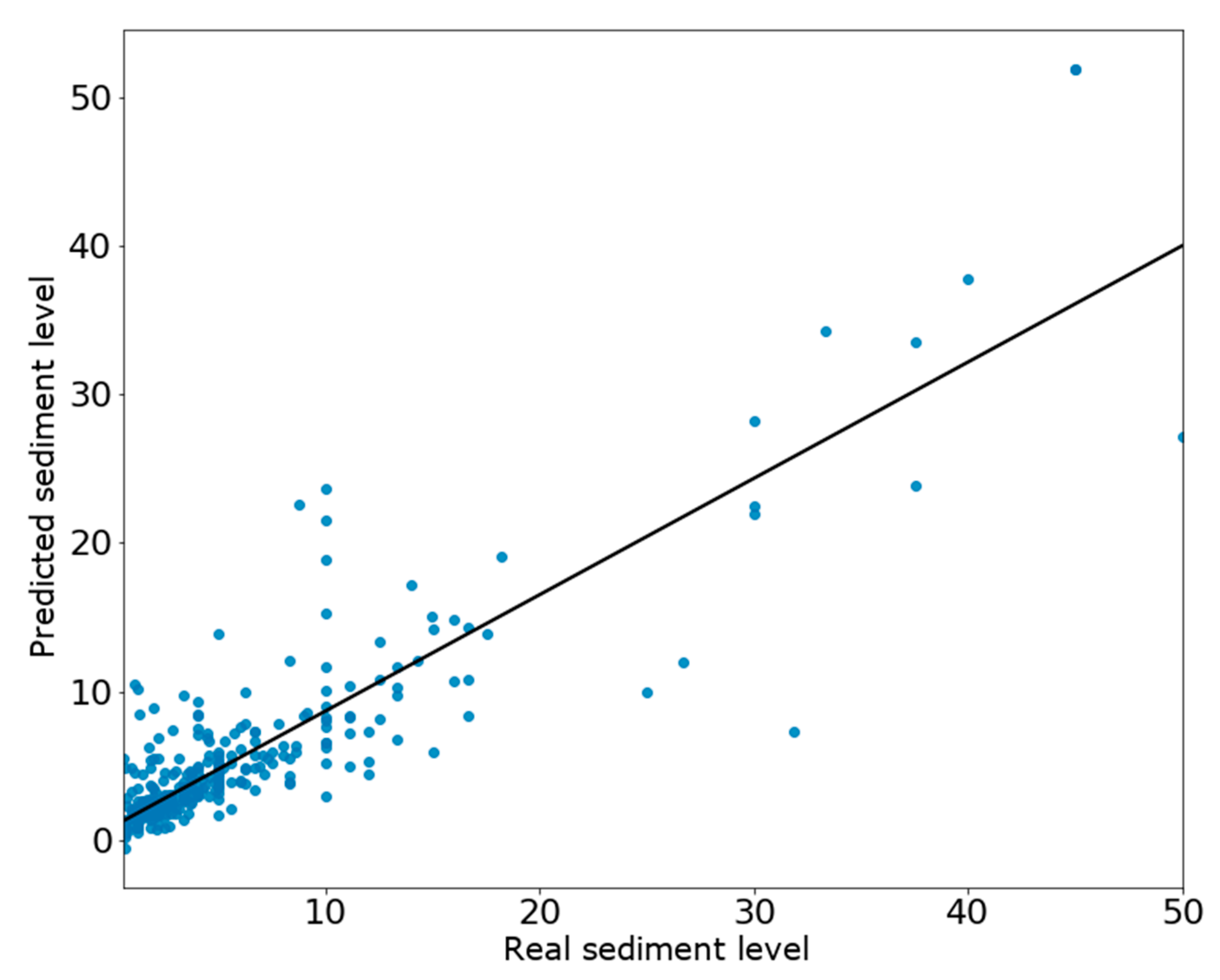
The ANN was the model which best worked for the first methodology, with an R² score of 0.76 being good enough [27] to recognize it as a model to use in this predicting methodology, a 1.5 MAE and an MSE value of 10.31. The scoring and the analyzed errors from Figure 2 indicate a good result that should be further improved in the future, adding more data in the training step, and optimizing the process of feature and hyperparameter selection.

Two models worked well for the third methodology, showing good scoring. The Gradient Boosting model classified better the cleaning cases, while the Extra Trees model perfectly classified the non-cleaning cases. Observe that it is more desirable to not miss any real cleaning needed, so it is better to have false positives than false negatives. Therefore, the Gradient Boosting model is the most suited to predict cleanings if the objective is to miss less critical situations in the sewer network.

The Gradient Boosting model performs better than other models reported in similar studies. The AUC of the model is good, with a value of 0.909, while in [15] the maximum tested model approaches an AUC of 0.71 using predictions of geographical aggregations. In the case of the condition of sanitary sewer pipes, Harvey and McBean [20,22] predicted an AUC of 0.77 and 0.85, respectively. The accuracy of the model was 88%, while in other studies involving the prediction of the condition in sanitary sewers [11,20,22] the accuracy was 0.62, 0.76, and 0.76, respectively. The recall has a lower scoring than in other studies, being 0.53 in this study, and 0.78 and 0.89 when predicting sewer condition [20,22].

It is also important to consider the imbalance of the datasets in the different studies to further compare the models. The test set used in this study contains 20% of positive registers (cleaning applied), while in other studies the imbalance is different. For example, in [17], different conditions are being predicted using a multiple-output classification and the imbalance variates on each condition, achieving the best prediction on the first condition, classifying 201 registers correctly out of 223, but unable to predict the fifth with three registers wrongly predicted. The imbalance in the data for this classification task could explain partly why the recall is so low, but this needs future analysis.

In the past, numerous studies modelled each section individually, and maintenance routines were not considered [14]. This study shows methodologies that use spatial features from near sections and information about the maintenance routines in the data model, providing a positive impact on the predictions.

The study can be used in the implementation of aid tools in Water and Sewerage companies. Predictions can provide important help in making decisions about section inspections. The predictions focused on the sediment level percentage offer an informative output that, although it does contain some error, it can provide enough data to make flexible decisions not only focused on cleaning routines. The binary classification predicts if the section pipe needs a cleaning looking at its past states, but the model does not consider other factors such as raining seasons or social events in the city. The output of the model should be considered as an indicator when managing the CSS.

5. Conclusions

Machine learning methods are suitable to predict sediment levels in CSS. From the studied methodologies, the predictions of the present situation in a section have proven to be more effective than the short-term predictions and the go-to. Furthermore, a model trained to predict the occupied percentage (or even the sediment level) in a short-term period requires the use of data in a small-time interval, meaning the increase of the number of inspections to do in a section, having to invest more money and resources. Moreover, this type of predictions needs to estimate the evolution of the sediment level taking into account rainy days and possible flash floods during the period. The addition of this data would increase the model scoring.

The Artificial Neural Network model is a clear winner when predicting the occupied percentage in a section, resulting in a focus point to study in the near future. With the addition of external features like pluviometry data, the expected results should improve.

Regarding the usefulness of our model in different scenarios, we should be careful with situations that show a different pattern of activity in cities. For example, the COVID-19 pandemic has affected society’s routine [28,29,30], and therefore models trained with past data will not be able to make such good predictions during this period. The impact of the pandemic on sewer systems is an important topic to study in the future, as is the creation of models that can adapt to this change.

References

1. Ashley, R.; Bertrand-Krajewski, J.-L.; Hvitved-Jacobsen, T. Sewer solids—20 years of investigation. Water Sci. Technol. 2005, 52, 73–84. [Google Scholar] [CrossRef] [PubMed]
2. Ashley, R.M.; Fraser, A.; Burrows, R.; Blanksby, J. The management of sediment in combined sewers. Urban Water 2000, 2, 263–275. [Google Scholar] [CrossRef]
3. Montserrat, A.; Bosch, L.; Kiser, M.; Poch, M.; Corominas, L. Using data from monitoring combined sewer overflows to assess, improve, and maintain combined sewer systems. Sci. Total. Environ. 2015, 505, 1053–1061. [Google Scholar] [CrossRef] [PubMed] [Green Version]
4. Del Mundo, D.M.N.; Sutheerawattananonda, M. Influence of fat and oil type on the yield, physio-chemical properties, and microstructure of fat, oil, and grease (FOG) deposits. Water Res. 2017, 124, 308–319. [Google Scholar] [CrossRef] [PubMed]
5. Corominas, L.; Garrido-Baserba, M.; Villez, K.; Olsson, G.; Cortés, U.; Poch, M. Transforming data into knowledge for improved wastewater treatment operation: A critical review of techniques. Environ. Model. Softw. 2018, 106, 89–103. [Google Scholar] [CrossRef]
6. Eggimann, S.; Mutzner, L.; Wani, O.; Schneider, M.Y.; Spuhler, D.; De Vitry, M.M.; Beutler, P.; Maurer, M. The Potential of Knowing More: A Review of Data-Driven Urban Water Management. Environ. Sci. Technol. 2017, 51, 2538–2553. [Google Scholar] [CrossRef] [PubMed] [Green Version]
7. Garrido-Baserba, M.; Corominas, L.; Cortés, U.; Rosso, D.; Poch, M. The Fourth-Revolution in the Water Sector Encounters the Digital Revolution. Environ. Sci. Technol. 2020, 54, 4698–4705. [Google Scholar] [CrossRef] [PubMed]
8. Blumensaat, F.; Leitão, J.P.; Ort, C.; Rieckermann, J.; Scheidegger, A.; Vanrolleghem, P.A.; Villez, K. How Urban Storm- and Wastewater Management Prepares for Emerging Opportunities and Threats: Digital Transformation, Ubiquitous Sensing, New Data Sources, and Beyond—A Horizon Scan. Environ. Sci. Technol. 2019, 53, 8488–8498. [Google Scholar] [CrossRef] [PubMed] [Green Version]
9. Therrien, J.-D.; Nicolaï, N.; Vanrolleghem, P.A. A critical review of the data pipeline: How wastewater system operation flows from data to intelligence. Water Sci. Technol. 2020, 82, 2613–2634. [Google Scholar] [CrossRef]
10. Arthur, S.; Crow, H.; Pedezert, L. Understanding blockage formation in combined sewer networks. Proc. Inst. Civ. Eng. Water Manag. 2008, 161, 215–221. [Google Scholar] [CrossRef]
11. Laakso, T.; Kokkonen, T.; Mellin, I.; Vahala, R. Sewer Condition Prediction and Analysis of Explanatory Factors. Water 2018, 10, 1239. [Google Scholar] [CrossRef] [Green Version]
12. Mohammadi, M.M.; Najafi, M.; Tabesh, A.; Riley, J.; Gruber, J. Condition Prediction of Sanitary Sewer Pipes. Pipelines 2019 2019, 117–126. [Google Scholar] [CrossRef]
13. Savic, D.A.; Giustolisi, O.; Laucelli, D.B. Asset deterioration analysis using multi-utility data and multi-objective data mining. J. Hydroinform. 2009, 11, 211–224. [Google Scholar] [CrossRef] [Green Version]
14. Cameron, B.; McGowan, M.; Mitchell, C.; Winder, J.; Kerr, R.; Zhang, M. Predicting Sewer chokeS through Machine Learning. Water E J. 2017, 2, 1–13. [Google Scholar] [CrossRef]
15. Bailey, J.; Harris, E.; Keedwell, E.; Djordjevic, S.; Kapelan, Z. Developing Decision Tree Models to Create a Predictive Blockage Likelihood Model for Real-World Wastewater Networks. Procedia Eng. 2016, 154, 1209–1216. [Google Scholar] [CrossRef] [Green Version]
16. Chughtai, F.; Zayed, T. Infrastructure Condition Prediction Models for Sustainable Sewer Pipelines. J. Perform. Constr. Facil. 2008, 22, 333–341. [Google Scholar] [CrossRef]
17. Salman, B.; Salem, O. Modeling Failure of Wastewater Collection Lines Using Various Section-Level Regression Models. J. Infrastruct. Syst. 2012, 18, 146–154. [Google Scholar] [CrossRef]
18. Ugarelli, R.; Kristensen, S.M.; Røstum, J.; Saegrov, S.; Di Federico, V. Statistical analysis and definition of blockages-prediction formulae for the wastewater network of Oslo by evolutionary computing. Water Sci. Technol. 2009, 59, 1457–1470. [Google Scholar] [CrossRef]
19. Syachrani, S.; Jeong, H.S.D.; Chung, C.S. Decision Tree–Based Deterioration Model for Buried Wastewater Pipelines. J. Perform. Constr. Facil. 2013, 27, 633–645. [Google Scholar] [CrossRef]
20. Harvey, R.R.; McBean, E.A. Comparing the utility of decision trees and support vector machines when planning inspections of linear sewer infrastructure. J. Hydroinform. 2014, 16, 1265–1279. [Google Scholar] [CrossRef] [Green Version]
21. Mashford, J.; Marlow, D.; Tran, H.D.; May, R. Prediction of Sewer Condition Grade Using Support Vector Machines. J. Comput. Civ. Eng. 2011, 25, 283–290. [Google Scholar] [CrossRef]
22. Harvey, R.R.; McBean, E.A. Predicting the structural condition of individual sanitary sewer pipes with random forests. Can. J. Civ. Eng. 2014, 41, 294–303. [Google Scholar] [CrossRef]
23. Wolpert, D.H.; Macready, W.G. No free lunch theorems for optimization. IEEE Trans. Evol. Comput. 1997, 1, 67–82. [Google Scholar] [CrossRef] [Green Version]
24. Goodwin, P.; Lawton, R. On the asymmetry of the symmetric MAPE. Int. J. Forecast. 1999, 15, 405–408. [Google Scholar] [CrossRef]
25. Fawcett, T. An introduction to ROC analysis. Pattern Recognit. Lett. 2006, 27, 861–874. [Google Scholar] [CrossRef]
26. Hanley, J.A.; McNeil, B.J. The meaning and use of the area under a receiver operating characteristic (ROC) curve. Radiology 1982, 143, 29–36. [Google Scholar] [CrossRef] [Green Version]
27. Hair, J.F.; Ringle, C.M.; Sarstedt, M. Partial Least Squares Structural Equation Modeling: Rigorous Applications, Better Results and Higher Acceptance. Long Range Plan. 2013, 46, 1–12. [Google Scholar] [CrossRef]
28. Rodríguez-Barranco, M.; Rivas-García, L.; Quiles, J.L.; Redondo-Sánchez, D.; Aranda-Ramírez, P.; Llopis-González, J.; Pérez, M.J.S.; Sánchez-González, C. The spread of SARS-CoV-2 in Spain: Hygiene habits, sociodemographic profile, mobility patterns and comorbidities. Environ. Res. 2021, 192, 110223. [Google Scholar] [CrossRef] [PubMed]
29. Aloi, A.; Alonso, B.; Benavente, J.; Cordera, R.; Echániz, E.; González, F.; Ladisa, C.; Lezama-Romanelli, R.; López-Parra, Á.; Mazzei, V.; et al. Effects of the COVID-19 Lockdown on Urban Mobility: Empirical Evidence from the City of Santander (Spain). Sustainability 2020, 12, 3870. [Google Scholar] [CrossRef]
30. Baldasano, J.M. COVID-19 lockdown effects on air quality by NO2 in the cities of Barcelona and Madrid (Spain). Sci. Total. Environ. 2020, 741, 140353. [Google Scholar] [CrossRef]
Figure 1. Bar plot of different identified elements in a sedimented section (x axis) and the number of appearances (y axis).
Sustainability 13 04013 g001
Figure 2. Resultant predictions from the ANN model using the test set. The line on the scatter plot represents the line of best fit, being a perfect score when the line goes from the bottom left to the top right, and the worse when it is completely flat.
Sustainability 13 04013 g002
Figure 3. Resultant predictions from the short-term ANN model using the test set.
Sustainability 13 04013 g003
Figure 4. Receiver operating characteristic (ROC) curve and area under the curve (AUC) on a test set (a) Gradient Boosting; (b) Extra Trees.
Sustainability 13 04013 g004
Figure 5. Confusion matrix computed on a test set (a) Gradient Boosting; (b) Extra Trees.
Sustainability 13 04013 g005