Abstract
The accessibility of transit stops (ATS) is a critical index for the evaluation of transit service, focusing on the first/last mile portions of transit trips. It is significantly affected by feeder modes, such as walking and cycling. Comparison of the application of different modes has been addressed in previous research, thus there is mostly only one feeder mode considered in this case study. This study has proposed a model for ATS with multiple feeder modes (ATSMFM), capable of integrating multiple feeder modes and considering the heterogeneity of travellers from the perspective of city managers. It is a bi-level model, combining cumulative and utility-based approaches. The final form of ATSMFM is developed referring to the cumulative approach, while the determination of the catchment area is utility-based. A numerical experiment has been conducted to demonstrate the necessity and applicability of ATSMFM. The results show that the ATS with a single feeder mode, such as cycling or walking, underestimates the catchment area of nearly one-third or two-thirds of travellers. As for ATSMFM, this proposed approach can automatically select the feeder mode from alternatives according to traveller attributes, thus removing the limitation of a single feeder mode, and is suitable for calculating ATS in the complex environment with multiple feeder modes. Besides, the ATSMFM model can support city managers with different emphases in transit planning via flexibly setting the threshold.
1. Introduction
Accessibility of transit stops (ATS) indicates the number of opportunities within the catchment area of transit services, focusing on the first/last mile portion of transit trips [1]. ATS is a critical index for the evaluation of transit service because the access/egress to/from the transit stop is a significant component of the transit trip [2,3]. It has been proved that high-quality ATS helps increase public transit usage [4,5,6,7,8,9,10]. Three aspects will affect the quality of ATS: the transit side (the deployment of transit stops), the feeder mode side, and the traveller side [11,12,13].
On the feeder mode side, the most commonly used feeder modes for bus transit are walking and cycling [12,14,15], as shown in Figure 1. Compared with walking, cycling can significantly enlarge the catchment area and increase the ATS, because cycling has a speed advantage over walking [12,16,17,18]. However, measurements of ATS with walking and cycling are usually studied separately, and there are few studies integrating walking, cycling, and other feeder modes in the evaluation of ATS.
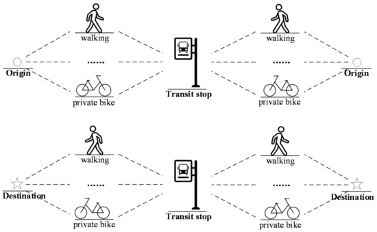
Figure 1.
Multiple feeder modes in accessing and egressing to/from the transit stop.
On the traveller side, studies have found that traveller attributes affect ATS. The catchment area of a transit stop is the spatial manifestation of ATS, within which people can access public transit service [13,19]. The size of the catchment area is found to vary with travellers of different socioeconomic attributes [12]. Besides, traveller attributes relate to the utility that travellers gain from public transit [13]. However, most studies ignore or use the average values of traveller attributes in calculating ATS [20,21,22,23]. There are a limited number of studies capturing the heterogeneity of traveller attributes when evaluating ATS [24,25,26].
There are three popular approaches for measuring accessibility: cumulative, gravity-based, and utility-based approaches. They have different strengths and focuses. Cumulative and gravity-based accessibility measures the number of opportunities within the accessible area, and they are from the perspective of planners or city managers [20]. The two approaches consider multiple travel modes by weighting travel modes based on a survey of travel mode split [27,28,29,30,31]. They are easy to understand in practice but neglect the relationship between travellers and accessibility [32]. On the other hand, utility-based accessibility measures the utility people can obtain from accessible activities or opportunities, and it is from the perspective of travellers by adopting the theory of traveller behaviour, which can consider various factors such as travel time, travel distance, travel cost, travel modes, and traveller attributes [24]. This approach considers multiple travel modes by integrating a travel mode choice model [33]. Utility-based accessibility measures the total surplus from the use of reachable opportunities, and it is difficult to understand without relatively complex theoretical knowledge of traveller behaviour [20,34,35].
This paper proposes a model for the ATS with multiple feeder modes by combining the cumulative and utility-based accessibility approaches. It is capable of integrating multiple feeder modes and considering traveller attributes in evaluating ATS, and is applicable for supporting city managers. A numerical experiment then is conducted to illustrate the necessity and applicability of multiple feeder modes included in ATS.
The remainder of this paper is organised as follows. Section 2 presents a literature review of the accessibility with multiple travel modes and accessibility to transit. Section 3 introduces the details of the ATSMFM model. Section 4 introduces the numerical experiment. Section 5 shows the results, and Section 6 presents the discussion. Section 6 gives a summary and identifies directions for future research. The symbols and abbreviations used in this paper are listed in Table A1 (Appendix A).
2. Literature Review
2.1. Accessibility of Transit Stops Approaches
There are three popular approaches for measuring the accessibility of transit stops: cumulative, gravity-based, and utility-based approaches.
The cumulative accessibility measures the number of opportunities within the catchment area of a transit stop [1,20,36,37]. Most studies define the catchment area as within 400 m from a bus stop and 800 m from a subway station [19,22,38,39,40,41]. Some studies have used 300 m or 800 m as the radius of a bus stop catchment area [13,42]. There is no standard distance threshold for the catchment area of the transit stop, generally ranging from 300 m to 1000 m. Moreover, the catchment radius is different for walking and cycling. For example, the 75th percentile travel distance from subway stations was 613 m with walking and 1579 m with cycling in Beijing [22]. The cumulative ATS usually only considers one travel mode in determining the catchment area [2,23]. Although some studies have compared the cumulative ATS with different feeder modes [43], in essence, they are still with a single feeder mode in each case and do not integrate multiple feeder modes in the calculation of ATS.
The gravity-based accessibility also counts the number of opportunities, but unlike the cumulative accessibility, it does not have a clear catchment concept. It discounts the number of opportunities located far from the origin using a decay function, so the gravity-based accessibility does not require a threshold to define the catchment area of a transit stop [21]. Cumulative and gravity-based approaches are from the perspective of planners and city managers, neglecting the relationship between travellers and accessibility [32].
Different from the cumulative and gravity-based accessibility, the utility-based accessibility measures the traveller’s ease in accessing/egressing to/from the transit stop [26]. It is a decision utility and includes a choice model in the calculation [44]. The built-in choice model in transit accessibility usually deals with the problem of choosing the trip destination and transit stop [24,25,26,45]. The utility-based accessibility has an advantage in a better understanding of traveller behaviour than the other two accessibility measures [25]. Most studies measure utility-based accessibility of transit from the perspective of the transit network and use walking as the only feeder mode [24,45]. Few studies have used the utility-based approach or integrating multiple feeder mode in measuring the ATS.
Table 1 summarizes these three approaches. By integrating the advantages of cumulative and utility-based approaches, a new approach for measuring ATS is explored in this paper, which is from the perspective of city managers and considers the heterogeneity of travellers in ATS.

Table 1.
Accessibility approaches and methods of considering multiple travel modes.
2.2. Methods of Considering Multiple Travel Modes in Accessibility
Studies have found that the travel mode can significantly affect the value of accessibility by comparisons of accessibilities with different travel modes [46,47]. An increasing number of studies have focused on accessibility with multiple travel modes [33,48], as shown in Table 1. There are two ways to consider multiple travel modes.
Firstly, researchers develop simple rules for choosing travel mode or use pre-defined travel-mode splits in the approaches of cumulative and gravity-based accessibility. The basic models are proposed by Shen [27] and Luo and Wang [28], considering the resource competition of travellers with different travel modes. The rules of choosing travel mode vary across studies. For example, Shen [27] let travellers choose travel modes according to motor vehicle ownership; Mao and Nekorchuk [29] divided travellers into travel-mode groups according to their travel distance; Xing et al. [30] and Lin et al. [31] assigned travel modes to travellers based on travel time by setting travel-time thresholds for different travel modes.
Secondly, researchers adopt the mode choice theory by using the utility-based accessibility approach from the perspective of travellers. The most frequently used mode choice model is the logit model with a strong assumption of irrelevance between alternative travel modes, but the result is of a closed form that is convenient for practical application [33,48,49,50,51].
These studies of accessibility with multiple travel modes show that considering multiple travel modes can make accessibility comprehensive. However, there are few studies considering multiple feeder modes in the calculation of ATS. This paper explores the ATS considering multiple feeder modes.
2.3. Influencing Factors to Accessibility of Transit Stops
The factors considered in calculating the accessibility with walking or cycling usually include travel mode, infrastructure, quality of paths, amenities, environmental factors, etc. [14,43,52,53,54,55,56]. Sometimes disability and the age of travellers are also considered in ATS [57]. Traveller attributes such as income have been proven to affect the size of a transit stop catchment area and the extent to which travellers rely on the transit service [13]. Finance is one crucial aspect of accessibility when considering traveller attributes, especially for low-income travellers [13,58,59,60]. One popular method to consider both travel cost and other factors in calculating accessibility is to convert other factors into generalised costs, such as monetising travel time by multiplying the travel time by the value of travel time. The value of travel time is usually specified to be the minimum hourly wage or estimated based on mode choice theory [36,37].
The way to consider these factors varies with accessibility approaches. For example, when considering the travel mode, cumulative and gravity-based accessibility only considers one travel mode or considers multiple travel modes by pre-setting the ratio of travel modes according to travel distance [27,29]. However, the utility-based approach can incorporate many more factors in the choice of travel modes, such as travel time, travel cost, and traveller income. Factors considered in the utility-based approach depend on its incorporated choice model. For example, the utility-based accessibility of transit network with choosing transit stops is not sensitive to transit fare, because the transit fare has no significant effect on the choice of transit stops for transit riders; thus, the model calibration weakens the influence of transit fare to travel utility [24].
Factors considered in the proposed model combines the factors in cumulative and utility-based approaches: travel time, travel distance, feeder mode, travel cost, and socioeconomic attributes.
3. Accessibility of Transit Stops with Multiple Feeder Modes
This section describes the proposed ATS model with multiple feeder modes (named the ATSMFM model). The ATSMFM model combines the cumulative approach and the utility-based approach into a bi-level model. The inputs, parameters, and outputs of this model are displayed in Table 2, and the model structure is depicted in Figure 2. This model can be used for both individuals and groups. The upper level of the ATSMFM model adopts the cumulative approach, which counts the number of opportunities within the catchment area. Different from the traditional cumulative approach, the catchment area herein is for an individual or a group, and it varies with traveller attributes. The lower level of the ATSMFM model supports the upper level with the catchment area defined by the utility-based approach.
Table 2.
The inputs, outputs and parameters of the proposed model of ATS with multiple feeder modes (ATSMFM).
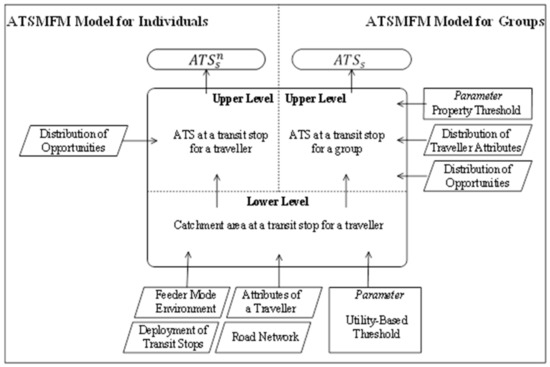
Figure 2.
Structure of the ATSMFM model.
3.1. Upper Level: Accessibility of Transit Stops for Individuals
The upper level adopted the approach of cumulative accessibility [20,36]. The ATS for individuals considers the heterogeneity of travellers, assuming that the catchment area varies with travellers with different attributes. In other words, whether an opportunity will be counted in the ATS depends on whether this opportunity is located in the specific catchment area of the traveller (individual catchment area, which is calculated by the lower level of the ATSMFM model). This part refines the ATS to each traveller, makes the ATS informative, and facilitates city managers to grasp the quality of public transit service for each type of travellers. The formula is as follows.
where is the value of ATS for the individual n at the transit stop s. is the number of opportunities (jobs or activities) in location j, and J is the set of locations near the transit stop s. is a dummy variable regarding the comparison between and , where is the travel distance between transit stop s and location j, and (determined by the lower level) is the catchment radius at stop s for individual n.
3.2. Upper Level: Accessibility of Transit Stops for Groups
In addition to the ATSMFM for individuals, this upper level provides another perspective: for groups. A specific transit stop services a group of travellers whose origins or destinations are near the transit stop. The attributes of the traveller group may vary with transit stops in different cities and even within different districts of a city. Therefore, the ATSMFM model adds this group perspective to help city managers evaluate ATS based on the group of travellers served.
The ATS of a group (denoted by ) is defined as the number of opportunities within the catchment area of stop s for the group. This catchment area for a group (group catchment area) is the largest area where the overlap rate of individual catchment areas is at least , as shown in Equation (6). This definition guarantees there are at least of individuals in the group believing that this group catchment area is reachable (or does not exceed their individual catchment area), as shown in Figure 3.
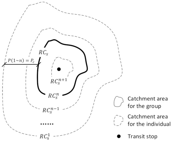
Figure 3.
Group catchment radius.
s.t.
where is a dummy variable regarding the comparison between and . denotes the radius of the group catchment area (group catchment radius), and RC is a variable of catchment radius. Here, the average value of is not used to determine the group catchment area, because the average value cannot reflect the variation of individual catchment areas. When the variation is large, the average value of cannot accurately represent the individual catchment areas of the group. N is the set of traveller group.
3.3. Lower Level: Determination of Catchment Area
As described in the upper level (Section 3.1 and Section 3.2), the individual catchment radius is the basis of the ATS calculation both for individuals and groups. The lower level of the ATSMFM model calculates to support the upper level. Previous studies usually used a certain travel time or distance as a threshold to determine the radius of the catchment area. In contrast, this paper uses a certain travel impedance (disutility) as a threshold to define the catchment area and allows each traveller to choose the feeder mode by incorporating a discrete choice model (Equation (9)). Specifically, is the maximal travel distance that the traveller can access/egress to/from the transit stop with the trip disutility less than the threshold , as expressed in Equations (8)–(12).
The individual catchment radius is the travel distance of the maximum travel impedance under certain conditions (Equation (8)). The conditions include the definition of travel impedance under the set of travel modes (Equation (9)), the definition of travel impedance with a particular travel mode (Equation (10)), and the condition of travel impedance threshold (Equation (11)). Equation (9) shows that the alternative with the lowest travel impedance is chosen, and the travel impedance under the set of travel modes is the expected minimum travel impedance associated with available travel modes; which is the definition of utility-based accessibility defined by Ben-Akiva and Lerman [61].
s.t.
where m is the indicator of a feeder mode, and M is the set of alternative feeder modes for transit. is the minimum travel impedance considering all alternative modes from s to j. is the travel impedance between location j and stop s for individual n with travel mode m, and it takes the form which consists of a deterministic part () and a random part (). is the observable component, and captures the uncertainty. is a utility-based threshold of the catchment area of traveller n, enabling the ATSMFM model to achieve the following three goals. Firstly, different from the traditional catchment area with a single travel mode, the utility-based threshold herein provides a unified threshold for various travel modes, allowing the model to adjust the travel mode in determining the catchment boundary based on the attributes of the traveller. Secondly, the threshold is utility-based, making it possible to comprehensively consider multiple factors and traveller attributes, while the traditional catchment boundary is only based on travel distance or time, and does not consider the heterogeneity of travellers. In this way, it can make the ATS comprehensive and informative to support city managers. Thirdly, the threshold can emphasise various aspects of accessibility and can be designed according to the goal of city managers, which makes the ATSMFM model flexible and adaptable for different objectives. The utility-based threshold can be set to a constant for all travellers. In this way, the boundary of the catchment area varies with travellers, but these boundaries have the same travel impedance. Another way is to set the utility-based threshold to vary with travellers; for example, it can be set as the travel impedance of walking a constant distance for each traveller. In this way, the catchment area boundary varies with travellers, but the boundary has the same walking effort.
When city managers only want to know the representative accessibility of each type of travellers, the travel impedance (Equation (10)) can be defined to be deterministic, ignoring the random term. According to this objective, there is no need to know the exact ATS of each traveller, and the representative term can satisfy the requirement. Besides, the representative disutility has an advantage in computation and can make the proposed model more applicable. A detail explanation of using representative disutility is presented in Appendix B.
4. Numerical Experiment
Numerical experiments were conducted to illustrate the applicability of the ATSMFM model. There were three scenarios of alternative feeder modes: Scenario 1, with only walking; Scenario 2, with only private bikes; and Scenario 3, with both walking and private bikes.
The considered area was the region within the 5th Ring Road of Beijing, China. Firstly, the model was specified to accommodate the scenarios of feeder modes. Secondly, traveller attributes were obtained from the datasets of resident income and transit smart card records.
4.1. Model Specification
This section specifies the lower level of the ATSMFM model and presents an analysis of the roles of vital variables.
4.1.1. Model Structure
The deterministic term of in Equation (10) is set to involve travel time and travel cost as Equation (13).
where is the value of travel time (VOT) of individual n, is the travel time between stop s and location j with mode m, and is the travel cost between stop s and location j by mode m.
The travel cost of walking is set to be zero. The travel cost of private-bike cycling adopts the calculation approach used by Song et al. [62]: is the cost of using an available private bike for one trip, evenly allocating the cost of owning a private bike to all its trips., where is the number of trips by private-bike cycling per day, and is the cost of owning a private bike for one day considering the purchase cost, maintenance cost, and lifespan of a bike. Then, the travel impedances with walking and private-bike cycling are expressed as follows.
where is the velocity of walking, is the velocity of private-bike cycling, and is the travel distance between bus stop s and location j. is assumed to have a Gumbel distribution, identically and independently across travellers and travel modes. In this case, is known as the “logsum” [61]:, where is a scale parameter of the distribution of , and because is disutility, therefore it is instead of . The variation of this distribution is , and equals the situation without the random term.
According to Equations (8), (14), and (15), the mapping relationship between and is derived. In Scenarios 1 and 2, there is only one alternative in the choice set, resulting in the term being equal to the deterministic part of travel impedance , so the corresponding catchment radius has nothing to do with the random term. However, in Scenario 3, there is more than one alternative, the corresponding catchment area related to the distribution of the random term, as shown in Equations (18) and (19). When considering the random term (Equation (18)), the catchment radius is a differentiable and monotonically increasing function of the utility-based threshold. However, when ignoring the random term (Equation (19)), the catchment radius is a piecewise linear function of the utility-based threshold, and it is continuous but not differentiable at the dividing point.
In Scenario 1:
In Scenario 2:
In Scenario 3:
4.1.2. Role of Value of Travel Time
The express role of is to convert travel time to an economic measure in the disutility function. According to the mapping relationship between the catchment radius and the travel impedance (Equations (16)–(18)), the role of the value of travel time is to reduce the marginal effect of catchment radius that increases with the threshold . The traveller with a large value of travel time has a small marginal catchment radius, and vice versa. As shown in Figure 4, the catchment radius curves with different values of travel time are of different gradients in all scenarios.
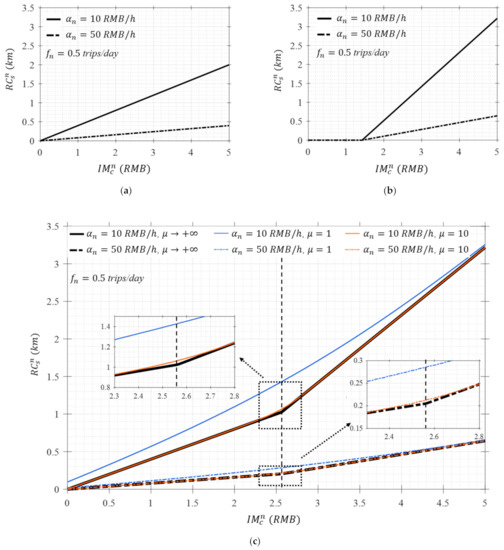
Figure 4.
Effect of the value of travel time on catchment radius. Scenario 1 (a), scenario 2 (b) and scenario 3 (c).
Figure 4c shows that as increases, the catchment radius curve becomes closer and closer to the curve of ignoring the random term. Under the utility-based threshold in the range of , there is a significant gap between the catchment radius with and that ignoring the random term. The gap between the catchment radius with and that of ignoring the random term is quite small, and it only exists near the dividing point.
4.1.3. Role of Bike Usage Frequency
The role of is to allocate the purchase cost and maintenance cost of a private bike to all trips of this bike. According to Equations (17) and (19), determines the dividing point of of the piecewise functions. A large corresponds to a dividing position with a small value in Scenarios 2 and 3, and vice versa. Figure 5 illustrates that curves have different dividing locations of , but they have the same gradient because is unrelated to the marginal . In Figure 5c, the effect of is the same as that in the analysis of Section 4.1.2.
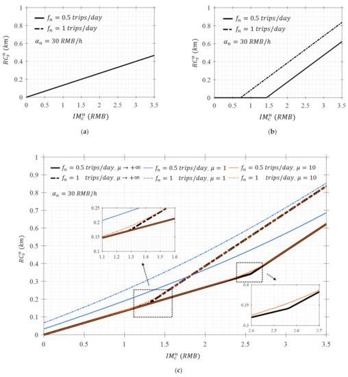
Figure 5.
Effect of bike usage frequency on catchment radius. Scenario 1 (a), scenario 2 (b) and scenario 3 (c).
4.2. Dataset
The considered traveller attributes include bike usage frequency and VOT. This section specifies the attribute distributions within the considered area in 2015. The smart card data were used to specify the distribution of transit-trip frequency for each traveller, and the income data released by Beijing Municipal Bureau Statistic were used to estimate the distribution of VOT.
4.2.1. Bike Usage Frequency
It was assumed that a private bike used to feed transit was used by only one person, the feeding trips accounted for 80% of all its trips, and a feeder bike can only serve a group of transit stops within a certain distance (set to be 0.5 km). Private-bike usage frequency of the traveller n at their stop-group g (denoted as ) equalled , where denotes the bus trip frequency of traveller n at the stop-group g (referred to as “bus trip frequency” for short). Besides, there were no bike racks on transit vehicles in Beijing.
The was calculated according to the smart card data of bus transit collected in October 2015 from Beijing Public Transit (the operator of all buses in Beijing). Passengers tap the smart card when boarding and alighting the bus. The smart card system recorded the card ID, boarding time, boarding stop, alighting time, alighting stop, and bus line of each trip. The collected data included 5,379,827 cardholders, whose origin or destination stops were within the considered area. There were 22,056,515 valid trips within five workdays. The was calculated with the procedure as shown in Figure 6, and Figure 7b plots its distribution. Due to the possibility of fare evasion and using the farebox instead of tapping a smart card, using the smart card records may underestimate the bus trip frequency to a certain degree [63].
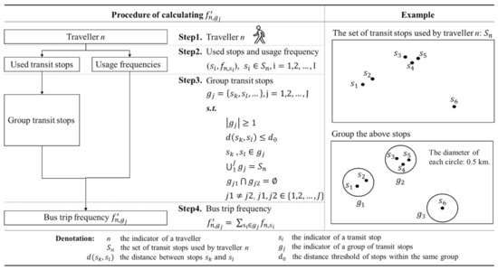
Figure 6.
Procedure of calculating bus trip frequency.
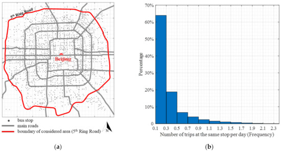
Figure 7.
Distribution of bus trip frequency within the 5th Ring Road of Beijing in 2015: considered area and bus stops (a) and distribution of bus trip frequency (b).
4.2.2. Value of Travel Time
VOT is a key indicator of willingness to pay for travel time, which considers the implicit trade-off between time and money, and it can be obtained from revealed preference data and stated preference data [64,65,66,67]. VOT varies with traveller income, travel mode, and travel purpose [68,69,70]. There is no standard method to determine the VOT, which is generally 20–200% of the income [66,67,71]. This paper set the VOT equal to traveller income.
The distribution of resident income was estimated using data released by Beijing Municipal Bureau Statistic. The released detailed-distribution data closest to 2015 were of 2017, therefore the distribution of income in 2015 was estimated by using the distribution data of 2017 (Figure 8a) and the income increase rate from 2015 to 2017 (Table 3). The estimation assumed that people with the same income level had the same income increase rate. The average income of urban residents in Beijing in 2015 was 25.3 RMB/h, and the estimated distribution in 2015 is shown in Figure 8b. The income distribution was skewed, and the percentage of people with income below the average was 67.7%.
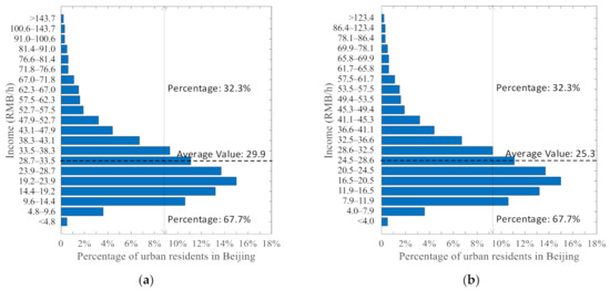
Figure 8.
Distribution of per capita disposable income of urban residents in Beijing: (a) 2017 and (b) 2015 (data source for 2017 (a): [73]).
Table 3.
Per capita disposable income of residents of Beijing (by income level) [72].
Assuming that the bus trip frequency and the value of travel time are independent, the joint distribution of these two attributions is illustrated in Figure 9.
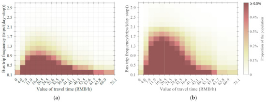
Figure 9.
Distributions of travellers (a) and bus trips (b) in Beijing.
4.3. Parameter Setup
However, in reality, travel time is affected by the quality of roads, the road slope, the age of the traveller, and many other factors [74,75]; due to the lack of data about these factors, the average walking speed (4 km/h) [76] and the average cycling speed (9 km/h) [77] were used as velocities of walking and cycling in the case study. According to the detailed structure of the cost of owning a private bike (Table 4), the parameter .
Table 4.
Cost structure of owning a private bike (adapted from Song et al. [62]).
The setting of a utility-based threshold is flexible. In the numerical experiment, two types of thresholds were set: (threshold I) and (threshold II). is the travel impedance of walking 400 m for traveller n:. It was selected as a type of threshold because the catchment area of 400 m from the transit stop is the most widely recognised value in studies. Under threshold I, the boundary of catchment areas varies with travellers, but these boundaries have the same walking effort for all travellers. On the other hand, is set to be a constant threshold, 2.5 RMB for all travellers. The value of 2.5 RMB was chosen because it is the average travel impedance of walking 400 m for travellers within the considered area where the average income is 25.3 RMB/h. The boundary of the catchment area varies with travellers, but these boundaries have the same travel impedance, 2.5 RMB.
The scale parameter of was set to be 2, and the corresponding standard deviation was 0.6413, which is equal to the expected travel impedance of 85 m walking for a traveller with a value of travel time of 30 RMB/h. Besides, the situation where the random term is ignored () was also considered.
As discussed in Section 3.2 is used to determine the catchment area of a traveller group at a transit stop. The experiment set nine values ranging from 10% to 90% to study the influence of on the results.
5. Results
This section presents the results of the numerical experiment in four parts. Section 5.1 and Section 5.2 show the individual catchment radius under two thresholds (determined by the lower level of the ATSMFM model). Section 5.3 introduces how the threshold impacts results. Section 5.4 shows the results of the group catchment radius and ATS under two thresholds (determined by the upper level of the ATSMFM model).
5.1. Individual Catchment Radius with Threshold I
Table 5 shows the results of the individual catchment radius. The individual catchment radius with threshold I was the same (400 m) for all travellers in Scenario 1, which is the same as the commonly used catchment radius in existing studies. Therefore, the result of Scenario 1 with the threshold I works as the benchmark. As shown in Figure 10a, the individual catchment radius in Scenario 2 increased along with the value of travel time and the bus trip frequency. There were 48.27% of travellers with the individual catchment radius being zero, because for these travellers, the cost of owning a private bike alone made the travel impedance exceed threshold I.
Table 5.
Results of the individual catchment radius.
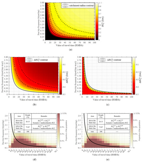
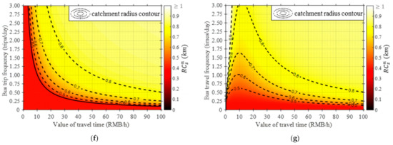
Figure 10.
Individual catchment radius with threshold I: (a) individual catchment radius in Scenario 2, (b) underestimation in Scenario 1, (c) underestimation in Scenario 2, (d) travellers with underestimated catchment radius, (e) trips corresponding to (d), (f) individual catchment radius in Scenario 3 with , (g) individual catchment radius in Scenario 3 with .
Figure 10b,c compare the results of Scenarios 1 and 2. Figure 10b shows that for travellers above the solid black line, the individual catchment radius with walking was 0 to 400 m lower than that with cycling. On the other hand, Figure 10c shows that for travellers below the solid black line, the individual catchment radius with private-bike cycling was 0 to 400 m lower than that with walking. Given the distribution of traveller attributes, 26.13% of travellers in Scenario 1 had a smaller catchment radius than in Scenario 2 (Figure 10d), and the bus trips of these travellers accounted for 49.33% of the total bus trips (Figure 10e). On the other hand, there were 73.87% of travellers in Scenario 2 having an underestimated catchment area (Figure 10d), and their bus trips accounted for 50.67% of the total bus trips (Figure 10e).
Scenario 3 considers both walking and private-bike cycling, as shown in Figure 10f,g. When ignoring the random term in travel impedance (), the individual catchment radius was 400 m for travellers below the solid black line, the same as that of walking. On the other hand, the individual catchment radius was bigger than 400 m for travellers above the solid black line, the same as the individual catchment radius of private-bike cycling. This solid black line is the dividing line between the feeder modes used to calculate the catchment radius. The ATSMFM model can automatically adjust the feeder mode according to the traveller attributes. As shown in Figure 10g, when considering the random term in travel impedance (), there was not a dividing line for mode choice, and the catchment radius is bigger than that with . As the variation of the random term decreases (the value of increases), the catchment radius is closer to that with .
5.2. Individual Catchment Radius with Threshold II
The individual catchment radius with threshold II varied with travellers in all three scenarios, as shown in Figure 11. In Scenario 1 (Figure 11a), the individual catchment radius decreased as the value of travel time increased, and had nothing to do with the bus trip frequency. This is because the travel impedance with walking had nothing to do with the bus trip frequency. In Scenario 2 (Figure 11b), for travellers with a bus trip frequency less than 0.23 trips per day, the individual catchment radius was equal to zero, because threshold II was less than the cost of owning a private bike for these travellers. For travellers whose bus trips frequency were greater than 0.23 trips per day, the individual catchment radius varied with traveller attributes. Figure 11c,d show the catchment radius in Scenario 3. When , the catchment area of multiple feeder modes is a simple integration of the catchment radius of a single feeder mode. However, as shown in Figure 11d, when is finite, the integration becomes complicated, and the catchment radius may be different from that of both Scenarios 1 and 2.
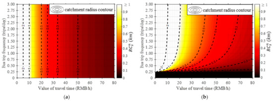
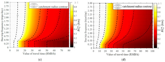
Figure 11.
Individual catchment radius with threshold II: (a) Scenario 1, (b) Scenario 2, (c) Scenario 3, , (d) Scenario 3, .
Figure 12a,b compare the results of Scenario 1 and 2. Figure 12a shows that for travellers with bus trip frequency higher than 0.41, the individual catchment radius with walking was 0 to more than 1000 m lower than that with private-bike cycling. On the other hand, Figure 12b shows that for travellers with bus trip frequency less than 0.41, the individual catchment radius with private-bike cycling was 0 to more than 1000 m lower than that with walking. Given the distribution of traveller attributes, 26.01% of travellers in Scenario 1 had a smaller individual catchment radius than in Scenario 2 (Figure 12c), and the bus trips of these travellers accounted for 54.81% of the total bus trips (Figure 12d). On the other hand, there were 73.99% of travellers in Scenario 2 having smaller individual catchment radiuses than in Scenario 1 (Figure 12c), and their bus trips accounted for 45.19% of the total bus trips (Figure 12d).
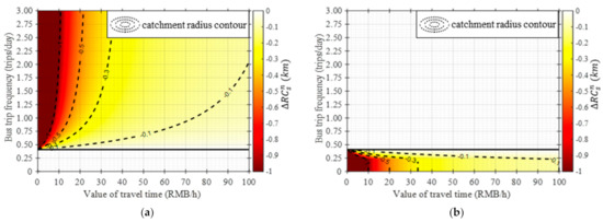
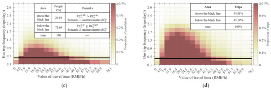
Figure 12.
Comparison of catchment radiuses with the threshold II: (a) underestimation in Scenario 1, (b) underestimation in Scenario 2, (c) travellers with underestimated catchment radius, (d) trips corresponding to (c).
Scenario 3 integrates Scenarios 1 and 2, as shown in Figure 10b. For travellers with a bus trip frequency less than 0.41 trips per day, the individual catchment radius was calculated based on walking, while for travellers with bus trip frequency greater than 0.41 trips per day, the individual catchment radius was calculated based on private-bike cycling.
5.3. Comparison of Individual Results under Two Thresholds
The results in Section 5.1 and Section 5.2 show that with both thresholds I and II, the individual catchment radius was significantly affected by the type of feeder mode. In the scenarios with only a single feeder mode, the catchment radius of some travellers was underestimated compared with other feeder modes, so ATS with a single feeder mode cannot well reflect the ATS with multiple feeder modes.
However, under the two thresholds, the correlations between the individual catchment radius and traveller attributes are different, as shown in Table 6. The two threshold settings make the changing trends of individual catchment radius different from or opposite to each other, which leads to different changing trends of ATSMFM under the two thresholds. When applying this ATSMFM model, the threshold should be designed according to specific objectives, and the setting method is not limited to the two methods used in this paper.
Table 6.
Relationship between the individual catchment radius and the traveller attributes.
5.4. Group Catchment Radius and ATS under Two Thresholds
Due to a lack of opportunity distribution data, this numerical experiment assumes that opportunities are distributed evenly in the considered area. In this way, the is proportional to the size of the catchment area. Therefore, this experiment uses the size of the catchment area to represent the value of (Table 7).
Table 7.
with different parameter settings.
As shown in Table 7, with threshold I, the group catchment radius in Scenario 1 is 400 m under all the nine values, because threshold I is defined as the travel impedance of walking 400 m, so all travellers have the same catchment radius herein.
The group catchment radius in Scenario 2 is zero for . This is because 48.27% of travellers with threshold I (travellers in the dark area in Figure 10a) and 41.44% of travellers with threshold II (in the dark area in Figure 11b) have a catchment radius equal to zero, so the group catchment radius remains equal to zero when with threshold I and with threshold II.
With and threshold I, the group catchment radius of Scenario 3 remains 400 m when . This is because 73.87% of travellers (travellers below the solid black line in Figure 10f) have a catchment radius equal to 400 m. The of Scenario 3 equals the corresponding in Scenario 1 when , and equals the corresponding in Scenario 2 when .
However, with threshold II, the in Scenario 3 is always bigger than the in Scenario 1 and the in Scenario 2. The ATS with multiple feeder modes is not just a simple splicing combination of ATS with different feeder modes, but an integration: the ATS with multiple feeder modes may be different from all the ATS with a single feeder mode.
The comparison of under the two thresholds in Scenario 3 is meaningless because their threshold settings emphasise different aspects. Threshold I emphasises the coverage of walking effort, and threshold II emphasises the coverage of economic cost.
6. Discussion
The results of the numerical experiment (Section 5) illustrate that this model can consider the heterogeneity of travellers and feeder modes in ATS, and its utility-based threshold can be adapted to support city managers with different goals. Besides, the ATSMFM model can calculate the ATS both for the individual and the group, making ATS more informative and directly related to the specific population served by the transit stop. There are three main limitations of this proposed model.
Firstly, this model is generalised. This paper does not provide a detailed description of how to construct all possible feeder modes in this model, because this paper focuses on the methodology. Possible feeder modes may include car driving, bus riding, electric-bike cycling, private-regular-bike cycling, shared-bike cycling, walking, etc. It is necessary to design the set of alternative feeder modes according to the actual situation and ensure that the model can distinguish these modes. The numerical experiment herein only regards private-bike cycling and walking. Future research could consider the modelling of other possible feeder modes, such as incorporating shared-bike cycling into the set of alternative feeder modes.
Secondly, the numerical experiment proposes two threshold settings. Future studies can explore other threshold settings to suit more scenarios and purposes.
Thirdly, though the ATSMFM model can provide a more comprehensive ATS, the calculation of ATS with this model is based on certain data, and the calculation process is more complicated than that of ATS with fixed travel time or distance of catchment radius (for example, 400 m). In the future, the calculation process can be modularised to unify input and output, making the model easier to apply.
7. Conclusions
ATS is a critical index for the evaluation of transit service, focusing on the first/last mile portion of transit trips. Studies have proven that the ATS is significantly affected by feeder modes and traveller attributes, but there are few studies integrating walking and cycling and considering traveller attributes in the evaluation of ATS. This study proposed a model of ATS with multiple feeder modes (ATSMFM), capable of integrating multiple feeder modes and considering the heterogeneity of travellers. The ATSMFM model can support city managers to formulate relative plans according to a complex feeder-mode environment and traveller attributes, which is consistent with people-oriented transportation planning.
A numerical study in Beijing was conducted to demonstrate the applicability of this ATSMFM model and clarified the process of the model in automatically adjusting the feeder mode according to the traveller attributes. Three scenarios of alternative feeder modes were set: Scenario 1, only walking; Scenario 2, only a private bike; and Scenario 3, both walking and a private bike. There are three main conclusions. Firstly, the results of Scenarios 1 and 2 showed the heterogeneity of catchment radiuses of travellers. The comparison between Scenarios 1 and 2 showed that the individual catchment radius varied significantly with different feeder modes. For some travellers, the difference of the individual catchment radius in Scenario 1 and 2 could reach more than 400 m, which is a great distance in the concept of the bus stop catchment area. Secondly, in the scenarios with only a single feeder mode, the catchment radius of some travellers was underestimated and cannot reflect the value in the real situation with multiple feeder modes. About 26% of travellers in Scenario 1 and about 74% of travellers in Scenario 2 had an underestimated individual catchment radius. Thirdly, the ATS with multiple feeder modes was not just a simple splicing combination of ATSs with different feeder modes, but an integration: the ATS with multiple feeder modes may be different from all the ATSs with a single feeder mode. For example, under threshold II, with two feeder modes with walking with private-bike cycling.
The threshold had a great influence on the results of the ATSMFM model. The two tested thresholds () not only led to different ATS values, but also changed trends of the ATS, or even made the values opposite to each other. When applying this ATSMFM model, the threshold should be designed according to specific objectives, and the setting method is not limited to the two methods used in this paper.
The proposed model is generalised, and it is necessary to design the set of alternative feeder modes according to the actual situation (the city’s traffic environment and the traveller attributes) and ensure that the model can distinguish these modes. Due to a lack of opportunity distribution data, this paper did not show the spatial distribution of in Beijing. In addition, to clearly discuss the mechanism of this model, the numerical study only considered private-bike cycling and walking, and did not include shared-bike cycling. Including bike-sharing into the set of alternative feeder modes would requires additional considerations, such as the availability of shared bicycles. Future studies can expand the set of alternative feeder modes to include shared-bike cycling.
Author Contributions
Conceptualization, M.S. and Y.Z. (Yi Zhang 1); methodology, M.S.; software, M.S.; validation, M.S., Y.Z. (Yi Zhang 2) and Y.Z. (Yi Zhang 1); formal analysis, M.S.; resources, M.L.; data curation, M.S.; writing—original draft preparation, M.S.; writing—review and editing, M.S., Y.Z. (Yi Zhang 1), M.L., and Y.Z. (Yi Zhang 2); visualization, M.S.; supervision, Y.Z. (Yi Zhang 1), M.L.; project administration, Y.Z. (Yi Zhang 2); funding acquisition, Y.Z. (Yi Zhang 2) and Y.Z. (Yi Zhang 1). All authors have read and agreed to the published version of the manuscript.
Funding
This work was supported in part by the National 135 Key Research and Development Program of China under Grant 2018YFB1600600, the National Natural Science Foundation of China under Grant 61673233, and the Shenzhen Science and Technology Program under Grant KQTD20170810150821146.
Institutional Review Board Statement
Not applicable.
Informed Consent Statement
Not applicable.
Data Availability Statement
Not applicable.
Conflicts of Interest
The authors declare no conflict of interest.
Appendix A
Table A1.
Description of symbols and abbreviations.
Table A1.
Description of symbols and abbreviations.
| Symbols | Explanation |
|---|---|
| ATS | Accessibility of transit stops |
| ATSMFM | Accessibility of transit stops with multiple feeder modes |
| Number of opportunities within the catchment area of stop s for the group | |
| Value of ATS for the individual n at the transit stop s | |
| Value of travel time (VOT) of individual n | |
| A dummy variable regarding the comparison between and | |
| A dummy variable regarding the comparison between and | |
| Corresponding vector of coefficients for | |
| Cost of owning a private bike for one day considering the purchase cost, maintenance cost, and lifespan of a bike | |
| Travel distance between transit stop s and location j | |
| Number of trips by private-bike cycling per day | |
| Private-bike usage frequency of the traveller n at their stop-group g | |
| Bus trip frequency of traveller n at the stop-group g (“bus trip frequency” for short) | |
| Utility-based threshold of the catchment area of traveller n | |
| Utility-based threshold I: the travel impedance of walking 400 m for traveller n | |
| Utility-based threshold II: a constant threshold,2.5 RMB for all travellers | |
| Minimum travel impedance considering all alternative modes from s to j | |
| Travel impedance between zone j and stop s for individual n with travel mode m | |
| Travel impedance between zone j and stop s for individual n by private-bike cycling | |
| Travel impedance between zone j and stop s for individual n by walking | |
| Indicator of a location | |
| Set of locations near the transit stop s | |
| Indicator of a feeder mode | |
| Set of alternative feeder modes for transit | |
| Indicator of a traveller | |
| Set of traveller group | |
| Number of opportunities (jobs or activities) in zone j | |
| Feeder mode: private-bike cycling | |
| Property threshold to define the boundary of the group catchment area | |
| RC | A variable of catchment radius |
| Group catchment radius | |
| Individual catchment radius at stop s for individual n | |
| Travel cost between stop s and location j for traveller n with mode m | |
| Travel cost of using an available private bike for one trip for traveller n | |
| Travel time between stop s and location j for traveller n with mode m | |
| VOT | Value of travel time |
| Velocity of walking | |
| Velocity of private-bike cycling | |
| Feeder mode: walking | |
| A vector of variables (such as travel time, travel distance, travel cost, comfort, etc.) affecting travel impedance of the trip between s and j with mode m |
Appendix B
The travel impedance is considered to be the disutility obtained by the traveller, and it can be defined as a representative disutility: for certain objectives, Equation (10) can ignore the random term.
In the theory of random utility maximisation [78], the usual form of random disutility is the sum of a representative term (a non-random term reflecting the representative disutility) and a random term (reflecting the idiosyncratic effect of unobserved variables during each choice occasion) [79,80]. The random utility is mostly used in the choice theory to analyse or predict the choice behaviour of consumers or travellers [79]. Compared with the result based on utility with only the representative term, the result based on the theory of random utility maximisation can better fit the choice of consumers or travellers.
However, different from the analysis of choice behaviour, the ATS is used for city managers, not needing to know the exact ATS of a single traveller. The objective of ATS is to support city managers to know the ATS for each kind of travellers with similar attributes and a group of travellers with different attributes, so they can make decisions according to the specific attributes of travellers within the considered area. We think that the purpose of ATS is to know what level of service people can access, not whether they ultimately choose this service. When there are several alternatives in calculating the level of service, the alternative that maximises the interested utility will be chosen to calculate the level of service. Therefore, the representative term can satisfy the requirement.
Secondly, representative disutility has an advantage in computation. The disutility with a random term will make the computation complex. Computation of the choice based on the representative disutility follows the principle of disutility minimisation to make a representative choice for each type of travellers, and it is easier than that with a random term. Although the logit-based logsum has been derived with a form which is easy to use, it is under the IIA (Independence of Irrelevant Alternatives) limitation [61]. When some alternatives are related, for example, when considering both private bicycles and shared bicycles, the logsum based on the nested logit model should be used.
Thirdly, only considering the representative term makes the proposed model more applicable. With a random term included in the disutility, detailed survey data are needed to estimate the parameters of the choice model, and the disutility is a relative value [24], making the physical meaning ambiguous. In contrast, only considering the representative term in the disutility has two advantages: (i) the disutility has a clear physical meaning, and city managers can set the physical meaning according to their objectives, for example, the disutility can be set to be the generalised cost; and (ii) the input data on traveller attributes can be coarse-grained or fine-grained. However, there is a disadvantage: the coefficient vector should be defined by experts.
References
- Moniruzzaman, M.; Páez, A. Accessibility to transit, by transit, and mode share: Application of a logistic model with spatial filters. J. Transp. Geogr. 2012, 24, 198–205. [Google Scholar] [CrossRef]
- Manout, O.; Bonnel, P.; Bouzouina, L. Transit accessibility: A new definition of transit connectors. Transp. Res. Part A Policy Pract. 2018, 113, 88–100. [Google Scholar] [CrossRef]
- Handley, J.C.; Fu, L.; Tupper, L.L. A case study in spatial-temporal accessibility for a transit system. J. Transp. Geogr. 2019, 75, 25–36. [Google Scholar] [CrossRef]
- Cervero, R.; Seskin, S. An evaluation of the relationships between transit and urban form. In TCRP Research Results Digest; Transportation Research Board: Washington, DC, USA, 1995; p. 7. Available online: https://onlinepubs.trb.org/onlinepubs/tcrp/tcrp_rrd_07.pdf (accessed on 15 February 2021).
- O’Sullivan, S.; Morrall, J. Walking distances to and from light-rail transit stations. Transp. Res. Rec. 1996, 1538, 19–26. [Google Scholar] [CrossRef]
- Hsiao, S.; Lu, J.; Sterling, J.; Weatherford, M. Use of geographic information system for analysis of transit pedestrian access. Transp. Res. Rec. 1997, 1604, 50–59. [Google Scholar] [CrossRef]
- Zhao, F.; Chow, L.-F.; Li, M.-T.; Ubaka, I.; Gan, A. Forecasting transit walk accessibility: Regression model alternative to buffer method. Transp. Res. Rec. 2003, 1835, 34–41. [Google Scholar] [CrossRef]
- Alshalalfah, B.; Shalaby, A.S. Case study: Relationship of walk access distance to transit with service, travel, and personal characteristics. J. Urban Plan. Dev. 2007, 133, 114–118. [Google Scholar] [CrossRef]
- Daniels, R.; Mulley, C. Explaining walking distance to public transport: The dominance of public transport supply. J. Transp. Land Use 2013, 6, 5–20. [Google Scholar] [CrossRef]
- El-Geneidy, A.; Grimsrud, M.; Wasfi, R.; Tétreault, P.; Surprenant-Legault, J. New evidence on walking distances to transit stops: Identifying redundancies and gaps using variable service areas. Transportation 2014, 41, 193–210. [Google Scholar] [CrossRef]
- Boarnet, M.G.; Giuliano, G.; Hou, Y.; Shin, E.J. First/last mile transit access as an equity planning issue. Transp. Res. Part A Policy Pract. 2017, 103, 296–310. [Google Scholar] [CrossRef]
- Flamm, B.J.; Rivasplata, C.R. Public transit catchment areas: The curious case of cycle-transit users. Transp. Res. Rec. 2014, 2419, 101–108. [Google Scholar] [CrossRef]
- Farber, S.; Marino, M.G. Transit accessibility, land development and socioeconomic priority: A typology of planned station catchment areas in the Greater Toronto and Hamilton Area. J. Transp. Land Use 2017, 10, 879–902. [Google Scholar] [CrossRef]
- Murray, A.T.; Davis, R.; Stimson, R.J.; Ferreira, L. Public transportation access. Transp. Res. Part D Transp. Environ. 1998, 3, 319–328. [Google Scholar] [CrossRef]
- Corazza, M.V.; Favaretto, N.J.S. A Methodology to Evaluate Accessibility to Bus Stops as a Contribution to Improve Sustainability in Urban Mobility. Sustainability 2019, 11, 803. [Google Scholar] [CrossRef]
- Zuo, T.; Wei, H.; Rohne, A. Determining transit service coverage by non-motorized accessibility to transit: Case study of applying GPS data in Cincinnati metropolitan area. J. Transp. Geogr. 2018, 67, 1–11. [Google Scholar] [CrossRef]
- Pritchard, J.P.; Tomasiello, D.B.; Giannotti, M.; Geurs, K. Potential impacts of bike-and-ride on job accessibility and spatial equity in São Paulo, Brazil. Transp. Res. Part A Policy Pract. 2019, 121, 386–400. [Google Scholar] [CrossRef]
- Zuo, T.; Wei, H.; Chen, N.; Zhang, C. First-and-last mile solution via bicycling to improving transit accessibility and advancing transportation equity. Cities 2020, 99, 102614. [Google Scholar] [CrossRef]
- Horner, M.W.; Murray, A.T. Spatial representation and scale impacts in transit service assessment. Environ. Plan. B Plan. Des. 2004, 31, 785–797. [Google Scholar] [CrossRef]
- Geurs, K.T.; Van Wee, B. Accessibility evaluation of land-use and transport strategies: Review and research directions. J. Transp. Geogr. 2004, 12, 127–140. [Google Scholar] [CrossRef]
- Geurs, K.T.; Östh, J. Advances in the measurement of transport impedance in accessibility modelling. Eur. J. Transp. Infrastruct. Res. 2016, 16. [Google Scholar] [CrossRef]
- Wang, Z.-J.; Chen, F.; Xu, T.-K. Interchange between metro and other modes: Access distance and catchment area. J. Urban Plan. Dev. 2016, 142, 04016012. [Google Scholar] [CrossRef]
- Ben-Elia, E.; Benenson, I. A spatially-explicit method for analyzing the equity of transit commuters’ accessibility. Transp. Res. Part A Policy Pract. 2019, 120, 31–42. [Google Scholar] [CrossRef]
- Nassir, N.; Hickman, M.; Malekzadeh, A.; Irannezhad, E. A utility-based travel impedance measure for public transit network accessibility. Transp. Res. Part A Policy Pract. 2016, 88, 26–39. [Google Scholar] [CrossRef]
- Berjisian, E.; Habibian, M. Walking Accessibility, Gravity-Based Versus Utility-Based Measurement. In Proceedings of the Transportation Research Board 96th Annual Meeting, Washington, DC, USA, 8–12 January 2017. [Google Scholar]
- Hasnine, M.S.; Graovac, A.; Camargo, F.; Habib, K.N. A random utility maximization (RUM) based measure of accessibility to transit: Accurate capturing of the first-mile issue in urban transit. J. Transp. Geogr. 2019, 74, 313–320. [Google Scholar] [CrossRef]
- Shen, Q. Location characteristics of inner-city neighborhoods and employment accessibility of low-wage workers. Environ. Plan. B Plan. Des. 1998, 25, 345–365. [Google Scholar] [CrossRef]
- Luo, W.; Wang, F. Measures of spatial accessibility to health care in a GIS environment: Synthesis and a case study in the Chicago region. Environ. Plan. B Plan. Des. 2003, 30, 865–884. [Google Scholar] [CrossRef]
- Mao, L.; Nekorchuk, D. Measuring spatial accessibility to healthcare for populations with multiple transportation modes. Health Place 2013, 24, 115–122. [Google Scholar] [CrossRef] [PubMed]
- Xing, L.; Liu, Y.; Liu, X. Measuring spatial disparity in accessibility with a multi-mode method based on park green spaces classification in Wuhan, China. Appl. Geogr. 2018, 94, 251–261. [Google Scholar] [CrossRef]
- Lin, J.-J.; Zhao, P.; Takada, K.; Li, S.; Yai, T.; Chen, C.-H. Built environment and public bike usage for metro access: A comparison of neighborhoods in Beijing, Taipei, and Tokyo. Transp. Res. Part D Transp. Environ. 2018, 63, 209–221. [Google Scholar] [CrossRef]
- Bhat, C.; Govindarajan, A.; Pulugurta, V. Disaggregate attraction-end choice modeling: Formulation and empirical analysis. Transp. Res. Rec. 1998, 1645, 60–68. [Google Scholar] [CrossRef]
- Zhang, T.; Dong, S.; Zeng, Z.; Li, J. Quantifying multi-modal public transit accessibility for large metropolitan areas: A time-dependent reliability modeling approach. Int. J. Geogr. Inf. Sci. 2018, 32, 1649–1676. [Google Scholar] [CrossRef]
- Koenig, J.-G. Indicators of urban accessibility: Theory and application. Transportation 1980, 9, 145–172. [Google Scholar] [CrossRef]
- Cascetta, E.; Cartenì, A.; Montanino, M. A new measure of accessibility based on perceived opportunities. Procedia-Soc. Behav. Sci. 2013, 87, 117–132. [Google Scholar] [CrossRef]
- El-Geneidy, A.; Levinson, D.; Diab, E.; Boisjoly, G.; Verbich, D.; Loong, C. The cost of equity: Assessing transit accessibility and social disparity using total travel cost. Transp. Res. Part A Policy Pract. 2016, 91, 302–316. [Google Scholar] [CrossRef]
- Ma, Z.; Masoud, A.R.; Idris, A.O. Modeling the Impact of Transit Fare Change on Passengers’ Accessibility. Transp. Res. Rec. 2017, 2652, 78–86. [Google Scholar] [CrossRef]
- O’Sullivan, D.; Morrison, A.; Shearer, J. Using desktop GIS for the investigation of accessibility by public transport: An isochrone approach. Int. J. Geogr. Inf. Sci. 2000, 14, 85–104. [Google Scholar] [CrossRef]
- Hunter-Zaworski, K. Transit Capacity and Quality of Service Manual; Transportation Research Board: Washington, DC, USA, 2003. [Google Scholar]
- Langford, M.; Fry, R.; Higgs, G. Measuring transit system accessibility using a modified two-step floating catchment technique. Int. J. Geogr. Inf. Sci. 2012, 26, 193–214. [Google Scholar] [CrossRef]
- Wang, S.; Sun, L.; Rong, J. Catchment area analysis of Beijing transit stations. J. Transp. Syst. Eng. Inf. Technol. 2013, 13, 183–188. [Google Scholar]
- Huang, D.; Liu, Z.; Fu, X.; Blythe, P.T. Multimodal transit network design in a hub-and-spoke network framework. Transp. A Transp. Sci. 2018, 14, 706–735. [Google Scholar] [CrossRef]
- Chandra, S.; Jimenez, J.; Radhakrishnan, R. Accessibility evaluations for nighttime walking and bicycling for low-income shift workers. J. Transp. Geogr. 2017, 64, 97–108. [Google Scholar] [CrossRef]
- Chorus, C.G.; De Jong, G.C. Modeling experienced accessibility for utility-maximizers and regret-minimizers. J. Transp. Geogr. 2011, 19, 1155–1162. [Google Scholar] [CrossRef]
- Nassir, N.; Hickman, M.; Malekzadeh, A.; Irannezhad, E. Modeling transit access stop choices. In Proceedings of the Transportation Research Board 94th Annual Meeting, Washington, DC, USA, 11–15 January 2015. [Google Scholar]
- Wachs, M.; Kumagai, T.G. Physical accessibility as a social indicator. Socio-Econ. Plan. Sci. 1973, 7, 437–456. [Google Scholar] [CrossRef]
- Dony, C.C.; Delmelle, E.M.; Delmelle, E.C. Re-conceptualizing accessibility to parks in multi-modal cities: A Variable-width Floating Catchment Area (VFCA) method. Landsc. Urban Plan. 2015, 143, 90–99. [Google Scholar] [CrossRef]
- Zhou, X.; Yu, Z.; Yuan, L.; Wang, L.; Wu, C. Measuring Accessibility of Healthcare Facilities for Populations with Multiple Transportation Modes Considering Residential Transportation Mode Choice. ISPRS Int. J. Geo-Inf. 2020, 9, 394. [Google Scholar] [CrossRef]
- Ben-Akiva, M. Disaggregate travel and mobility choice models and measures of accessibility. In Behavioural Travel Modelling; Hensher, D.A., Storper, P.R., Eds.; Croom Helm: London, UK, 1979; pp. 654–679. [Google Scholar]
- Train, K. A structured logit model of auto ownership and mode choice. Rev. Econ. Stud. 1980, 47, 357–370. [Google Scholar] [CrossRef]
- Hoorn, T.V.D. The logsum as an evaluation measure: Review of the literature and new results. Transp. Res. Part A Policy Pract. 2007, 41, 874–889. [Google Scholar]
- Parks, J.R.; Schofer, J.L. Characterizing neighborhood pedestrian environments with secondary data. Transp. Res. Part D Transp. Environ. 2006, 11, 250–263. [Google Scholar] [CrossRef]
- Stewart, O.T.; Moudon, A.V. Using the built environment to oversample walk, transit, and bicycle travel. Transp. Res. Part D Transp. Environ. 2014, 32, 15–23. [Google Scholar] [CrossRef]
- Etminani-Ghasrodashti, R.; Ardeshiri, M. The impacts of built environment on home-based work and non-work trips: An empirical study from Iran. Transp. Res. Part A Policy Pract. 2016, 85, 196–207. [Google Scholar] [CrossRef]
- Lakhotia, S.; Rao, K.R.; Tiwari, G. Accessibility of Bus Stops for Pedestrians in Delhi. J. Urban Plan. Dev. 2019, 145, 05019015. [Google Scholar] [CrossRef]
- Barabino, B. Automatic recognition of “low-quality” vehicles and bus stops in bus services. Public Transp. 2018, 10, 257–289. [Google Scholar] [CrossRef]
- Lin, T.G.; Xia, J.; Robinson, T.P.; Goulias, K.G.; Church, R.L.; Olaru, D.; Tapin, J.; Han, R. Spatial analysis of access to and accessibility surrounding train stations: A case study of accessibility for the elderly in Perth, Western Australia. J. Transp. Geogr. 2014, 39, 111–120. [Google Scholar] [CrossRef]
- Penchansky, R.; Thomas, J.W.J.M.C. The concept of access: Definition and relationship to consumer satisfaction. Med. Care 1981, 19, 127–140. [Google Scholar] [CrossRef]
- Carruthers, R.; Dick, M.; Saurkar, A. Affordability of public transport in developing countries. The World Bank: Washington, DC, USA, 2005. [Google Scholar]
- Saurman, E. Improving access: Modifying Penchansky and Thomas’s theory of access. J. Health Serv. Res. Policy 2016, 21, 36–39. [Google Scholar] [CrossRef] [PubMed]
- Ben-Akiva, M.; Lerman, S. Discrete Choice Analysis: Theory and Application to Travel Demand; The MIT Press: Cambridge, UK, 1985. [Google Scholar]
- Song, M.; Wang, K.; Zhang, Y.; Li, M.; He, Q.; Zhang, Y. Impact Evaluation of Bike-Sharing on Bicycling Accessibility. Sustainability 2020, 12, 6124. [Google Scholar] [CrossRef]
- Barabino, B.; Lai, C.; Olivo, A. Fare evasion in public transport systems: A review of the literature. Public Transp. 2020, 12, 27–88. [Google Scholar] [CrossRef]
- Mackie, P.J.; Jara-Dıaz, S.; Fowkes, A. The value of travel time savings in evaluation. Transp. Res. Part E Logist. Transp. Rev. 2001, 37, 91–106. [Google Scholar] [CrossRef]
- Hess, S.; Bierlaire, M.; Polak, J.W. Estimation of value of travel-time savings using mixed logit models. Transp. Res. Part A Policy Pract. 2005, 39, 221–236. [Google Scholar] [CrossRef]
- Small, K.A. Valuation of travel time. Econ. Transp. 2012, 1, 2–14. [Google Scholar] [CrossRef]
- Liu, Y.; Gu, T.; Zhou, L.; Sun, M. SP Survey Design Based on Travel Time Value of Residents. Urban Transp. China 2018, 16, 76–82. [Google Scholar]
- Qi, T.; Liu, D.; Liu, Y. A study of the traveling time cost of Beijing residents. J. Highw. Transp. Res. Dev. 2008, 25, 144–146. [Google Scholar]
- Athira, I.; Muneera, C.; Krishnamurthy, K.; Anjaneyulu, M. Estimation of value of travel time for work trips. Transp. Res. Procedia 2016, 17, 116–123. [Google Scholar] [CrossRef]
- Kouwenhoven, M.; de Jong, G. Value of travel time as a function of comfort. J. Choice Model. 2018, 28, 97–107. [Google Scholar] [CrossRef]
- Qin, P.; Chen, Y.A.; Xu, J.T. Travel Behavior Analysis for the Residents in Beijing: Value of Time and Travel Demand Elasticity Estimates. Econ. Geogr. 2014, 34, 17–22. [Google Scholar]
- Beijing Municipal Bureau Statistics; Beijing Statistical Yearbook. People’s Living Conditions; China Statistics Press: Beijing, China, 2019.
- Beijing Municipal Bureau Statistics. Sharing the Fruits of Economic Development-Residents’ Income has Grown Steadily. Available online: http://tjj.beijing.gov.cn/zt/dgsdzxp/msgs/201811/t20181105_146334.html (accessed on 11 November 2018).
- Pezzagno, M.; Tira, M. Town and Infrastructure Planning for Safety and Urban Quality: Proceedings of the XXIII International Conference on Living and Walking in Cities (LWC 2017), 15–16 June 2017, Brescia, Italy; CRC Press: Boca Raton, FL, USA, 2018. [Google Scholar]
- Zazzi, M.; Ventura, P.; Caselli, B.; Carra, M. GIS-based monitoring and evaluation system as an urban planning tool to enhance the quality of pedestrian mobility in Parma. In Town and Infrastructure Planning for Safety and Urban Quality: Proceedings of the XXIII International Conference on Living and Walking in Cities; CRC Press: Boca Raton, FL, USA; Taylor and Francis Group: London, UK, 2018. [Google Scholar]
- Millward, H.; Spinney, J.; Scott, D. Active-transport walking behavior: Destinations, durations, distances. J. Transp. Geogr. 2013, 28, 101–110. [Google Scholar] [CrossRef]
- Mobike, Bike-sharing and the city: 2017 white paper. 2017. Available online: https://mobike.com/global/public/Mobike%20-%20White%20Paper%202017_EN.pdf (accessed on 15 February 2021).
- McFadden, D.; Train, K. Mixed MNL models for discrete response. J. Appl. Econom. 2000, 15, 447–470. [Google Scholar] [CrossRef]
- McFadden, D. Conditional logit analysis of qualitative choice behavior. In Frontiers in Econometrics; Zarembka, P., Ed.; Academic Press: New York, NY, USA, 1973. [Google Scholar]
- Bhat, C.R.; Sardesai, R. The impact of stop-making and travel time reliability on commute mode choice. Transp. Res. Part B Methodol. 2006, 40, 709–730. [Google Scholar] [CrossRef]


Publisher’s Note: MDPI stays neutral with regard to jurisdictional claims in published maps and institutional affiliations. |
© 2021 by the authors. Licensee MDPI, Basel, Switzerland. This article is an open access article distributed under the terms and conditions of the Creative Commons Attribution (CC BY) license (http://creativecommons.org/licenses/by/4.0/).