Abstract
The barrier layer (BL) is a layer of water separating the thermocline from the density mixed layer in the upper ocean, which has the capability of reducing the negative feedback effect caused by tropical cyclone (TC) acting on the upper ocean and back on the TC itself. This study analyzed in-situ Argo floats measurements, data-assimilated HYCOM/NCODA reanalysis, and the longer-term (1961–2010) variations of Ocean Reanalysis System 4 (ORAS4) based BL in the TC main development region (MDR) to characterize the BL in the western North Pacific (WNP) for different temporal scales and to understand its role in resisting TC induced sea surface cooling. First, the result indicates that the effect of BL on TC enhancement in the MDR of WNP might be overestimated. Further analysis based on partial correlation shows that the BL plays a key role in resisting the cooling response only while BL is strong (BL thickness ≥ 5 m) and TC wind forcing is weak. Meanwhile, the distribution of BL demonstrates markedly the mesoscale characteristic. BL with thickness 0–5 m occupies the highest proportion (~67.55%), while thicker BL (BL thickness (BLT) larger than 5 m) takes up about 25–30%. Besides, there are ~3% with BL thicker than 30 m. For life length, BLT with 0–5 m is limited to 5 days, while BL with thickness more than 30 m can persist for more than 30 days. The scenario is attributed to diverse processes that result in different characteristic temporal scales of BL. Additionally, the analysis of coverage region and average BLT in the recent decade shows a serious situation: both the spatial coverage and BLT increase sharply from 2001 to 2010, which implies that TC–BL interactions might occur more frequently and more vigorously in future if the changing trend of BL remains unchanged.
1. Introduction
Interaction between tropical cyclone (TC) and the upper ocean structure has been well investigated in the past decades [1,2,3,4,5]. Since the ocean is the energy source supplying heat fluxes (latent heat fluxes, sensible heat fluxes) for TC enhancement, the studies of pre-existing oceanic conditions along the TC tracks are important in improving the forecasts of TC intensity development [6]. Despite the fact that TC intensity can be enhanced by drawing energy from the ocean while passing the favorable pre-existing oceanic conditions (such as high ocean heat content or warm mesoscale eddy), the violent wind field of TC often stirs up colder water below, destroying these warmer upper ocean structures, and results in the sea surface temperature (SST) cooling effect (i.e., negative feedback effect). The TC-induced SST cooling effect is mainly associated with entrainment and upwelling processes while the translation speed of TC determines which process should be dominant [7].
However, some upper ocean structures may have the capability of reducing the negative feedback effect, which is discussed in previous studies [8,9,10]. Among these pre-existing upper ocean structures, the ocean BL is a relatively less studied feature. The BL is a layer of water separating the thermocline from the density mixed layer in the upper ocean [11]. In some regions, especially the tropical oceans, a low-salinity layer is situated on the surface where the uniform density mixed layer becomes shallower than the isothermal layer, and thus a salinity barrier layer is formed [11]. In the meantime, the upper ocean is divided into the mixed layer, the BL, and the thermocline into three layers. In this situation, the increased stratification and stability within the layers reduces storm-induced vertical mixing and sea surface temperature cooling when a TC passes over regions with BLs. This causes an increase in enthalpy flux from the ocean to the atmosphere and, consequently, a possible intensification of TC [8]. Meanwhile, heavy rainfall might lead to the generation of BL, because the uniform density mixed layer becomes shallower than the uniform temperature isothermal layer due to salinity influence. Subsequently, the BL would act as a barrier to vertical mixing and influence the stratification eventually [8,11]. Besides, the barrier layer thickness (BLT) is the difference between the isothermal layer depth (ILD) and mixed layer depth (MLD), which can be briefly interpreted as ILD minus MLD (see Figure 1). In other words, BL appears when density stratification emerges in the isothermal layer, i.e., Equation (1),
where ρ is water density, T is temperature, S is salinity, and z is water depth. Since the BL is part of the isothermal layer, the temperature gradient in the BL is relatively small. Therefore, water density stratification in the BL is generally thought to be mainly controlled by the salinity gradient [12]. This brings along the more stable water column within the BL range. More precisely, the Richardson number (Equation (2)),
where is the gravity, is the water density, and is the horizontal layer velocity, will be larger under the same velocity shear condition if the vertical density gradient exists. A high Richardson number results in a stabilized and stratified water column which reduces the gradient mixing and the entrainment mixing. The area with the existence of BL thus commonly maintains a higher SST than the area without it after the stir of storm wind field.
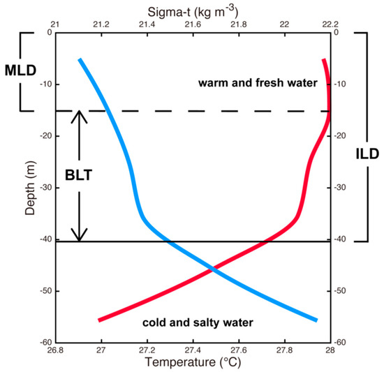
Figure 1.
An illustration of the temperature (red line) and the density (blue line) profile. The solid line and the dashed line indicate the isothermal layer depth (ILD) and mixed layer depth (MLD) respectively. The barrier layer (BL) is then defined as the layer between the ILD and the MLD (Profiles data were retrieved from European Centre for Medium-Range Weather Forecasts (ECMWF) Ocean Reanalysis System 4 (ORAS4)).
Studies about factors related to TC development and enhancement are important and beneficial for improving the accuracy of TC intensity forecast while facing the threat of TC invasion. The western North Pacific (WNP) has been the most active TC basin in recent decades [13]. Moreover, the climatological composite of BLT during the TC-prevailing season (July–November in the northern hemisphere and December–April in the southern hemisphere) in the tropics reveals that the WNP TC-prevailing season matches the wide range of BL coverage (Figure 2). This consistence makes the WNP TC main development region (MDR) an ideal region for studying the TC-BL interaction (the MDR only refers to the MDR at the WNP afterward).
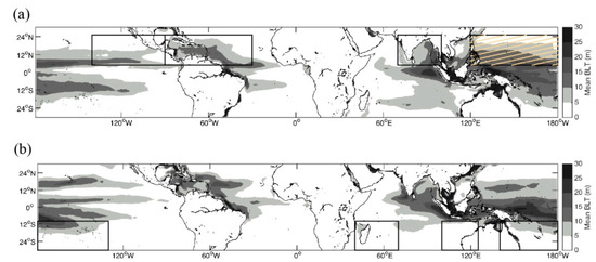
Figure 2.
Composite climatology of BL spatial distribution in global tropical area (30° N–30° S) of (a) July to November and (b) December to April in the period of 1961–2010, which represent the TC-prevailing seasons in the northern hemisphere and the southern hemisphere respectively. Black line boxes indicate several global TC main development regions and the WNP area is covered by yellow slants (data from ORAS4).
Previous studies of the BL and TC intensification show controversial results. Some studies suggest that the BL is favorable for TC intensification, whereas others demonstrate that the BL has little impact. The diversity was thought to be associated with the mesoscale characteristics and different temporal scales of BL as demonstrated in this study. In order to examine the characteristic of BL in the WNP and its contribution to TC enhancement, this study first generalizes the statistics of the capability of BL in resisting the sea surface cooling induced by TC and then focuses on the longer-term (1961–2010) variation of BL in the MDR. Additionally, previous studies [14,15] pointed out that BLs in the subtropical ocean possess mesoscale characteristics with a life length of less than 10 days both on temporal and spatial scales. Therefore, the changing trend of average thickness and life length of transient BLs are investigated simultaneously. The data and methods are introduced in Section 2. Statistics of BL impact on TC enhancement is shown in Section 3.1. Mesoscale BL characteristics and changing trends are demonstrated in Section 3.2. Temporal and spatial variations in interannual temporal scale are presented in Section 3.3. Also, possible dynamics leading to interannual BL variability are also unveiled and discussed. Finally, conclusion and discussions are presented in the final Section.
2. Materials and Methods
The primary data used in this study is obtained from the European Centre for Medium-Range Weather Forecasts (ECMWF) Ocean Reanalysis System 4 (ORAS4, [16]), which includes several monthly mean physical variables (temperature, salinity, velocities, isothermal/mixed layer depth) on a 1 × 1 global grid. This study employs the ORAS4 data from 1961 to 2010 in the climate scale analysis of BL variability. Argo floats in-situ data [17] from 2001 to 2010 were used to compute the mean temperature, salinity and density profiles for different BL formations including their location, which enabled us to compile statistics on the relationship between BL and consequential TC-induced SST cooling. Besides, the Argo floats data is also utilized for validating the HYCOM/NCODA 1/12 global daily reanalysis (GLBu0.08, https://www.hycom.org/dataserver/, accessed on 28 May 2020 [18]), which is analyzed to reveal the mesoscale characteristics of BL. Both the Argo floats and HYCOM data are interpolated at an interval of 5 m with Akima spline method primarily [19]. All the tropical cyclone best track data are obtained from Joint Typhoon Warning Center (JTWC). The data includes TC center position (per 6 h), maximum wind speed, minimum sea level pressure etc. A non-dimensional parameter, , where is the TC translational speed (computed from TC center position data); is the Coriolis parameter, and is the TC length scale defined as 100 km, is adopted to separate the slow-moving TCs () from the fast-moving TCs () in the statistical analysis [20,21].
The density in the upper ocean, which is defined as above 200 m depth in this work, is calculated via the Equation of State of Seawater. The equation of state was defined by the Joint Panel on Oceanographic Tables and Standards (UNESO, 1981) by fitting available measurements with a standard error of 3.5 ppm for pressure up to 1000 bars, for temperatures between freezing and 40 °C, and for salinities between 0 and 42 [22]. The density ρ (in kilograms per cubic meter) is expressed in terms of pressure p (in bars), temperature t (in °C), and practical salinity S. With accurate measurements of temperature, salinity, and pressure, the equation can be used to determine density very accurately. The complete form of equation of state can be seen in Gill [22]. Here, density is determined using the temperature and salinity data from the ORAS4, HYCOM, and Argo floats. On the other hand, the method of computing BL and BLT is defined in the Equations (3)–(6) below,
where T10 (°C) and S10 (kg m−3) represents the temperature and salinity at 10 m underwater, respectively. The threshold (Δσ, density) of MLD can be computed with the two variables while neglecting the pressure effect. Consequently, ILD is the depth where the water temperature decreases by 0.2 °C compared to T10, and the criterion of MLD is similar but at the depth where the water density increases by Δσ compared to σ10. Moreover, the BL density profiles above 30 m depth must be strictly increasing for the purpose of preventing unstable cases from being defined as BL mistakenly. All the monthly mean gradients of temperature or salinity are estimated by the first order forward difference. Partial correlation (using the matrix inversion method) and multiple regression are used in analyzing the particular influence of different variables on the process of TC induced sea surface cooling and in climate scale BL analysis. Finally, the two-tailed Student’s t-test is applied to all the correlation statistical tests. Hypothesis test of the significance of the correlation coefficient can help to decide whether the linear relationship is strong.
Isothermal Layer Depth (ILD) = Depth (T10 − 0.2 °C)
Density Mixed Layer Depth (MLD) = Depth (σ10 + Δσ)
Δσ = σ (T10 − 0.2 °C, S10, 0) − σ (T10, S10, 0)
BLT = ILD − MLD
3. Results
3.1. Possible Linkage between BL and Consequential TC Triggered Sea Surface Cooling
TC-BL events that occurred in 2001–2010 are analyzed using Argo floats and JTWC data to evaluate the BL capability in resisting the sea surface cooling induced by the TC. The TC events are separated into the Tropical Storm (TS) category and above TS category (Category 1 to Category 5) according to the Saffir–Simpson hurricane scale (SSHS). The SSHS classifies hurricanes (tropical cyclones) that exceed the intensities of tropical depressions and tropical storms into five categories distinguished by the intensities of their sustained winds. The central position of the TC (sampled every 6 h) is considered as the origin, and the average cooling of SST (ΔT at 10 m depth) of the surrounding area (region covering 3 × 3 box) is computed from the temperature difference between the 10-day average (day 11 to day 2) prior to the TC-passage and the second day (day + 2) after. Besides the BLT, the other important factors responsible for TC-induced surface cooling include a depth of 26 °C isotherm (D26) which represents the warm subsurface structure, TC wind speed, and TC translational speed, which are also chosen as independent variables in the partial correlation with ΔT.
Among the different TC-induced cooling processes, Ekman pumping and vertical mixing (entrainment cooling) are regarded as the two main mechanisms which are generated by slow-moving TC and fast-moving TC separately. In addition to the non-dimensional parameter, the ratio between TC translational speed and phase speed of the ocean first baroclinic mode (i.e., Froude number) is also reported to be a threshold for differentiating the above two mechanisms [23]. Therefore, TCs which possess both and a translational speed of less than 2.5 ms−1 (the same as the average phase speed of the first baroclinic mode in the northern hemisphere, [24]) are defined as slow-moving cases and are excluded from the analysis, but are still showed with cross marks in Figure 3.
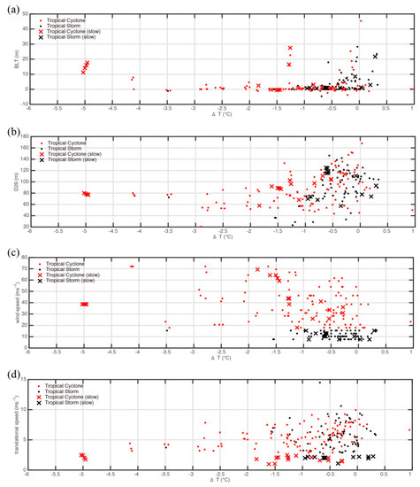
Figure 3.
Scatter diagrams of four chosen variables, which are (a) BL thickness (BLT), (b) 26 °C isotherm (D26), (c) wind speed, (d) translational speed, and the sea surface cooling effect, ΔT. Historical records of tropical cyclones (TCs) and tropical storms (TSs) from Joint Typhoon Warning Center (JTWC) are divided into a relatively fast group and a relatively slow group according to the translational speeds and non-dimensional parameter , and are symbolized by dot marks and cross marks separately.
Warm subsurface layer, low wind speed, and high translational speed provides favorable conditions for minimal surface cooling after the TC passage ([1,4,9,20,21,23]). These expected relations are reproduced from the statistical analysis on average as shown in Figure 3b–d. Also, the slow-moving TC cases hold the larger SST cooling than the relatively fast-moving cases under the same conditions. Meanwhile, most of the ΔT inversions occur with the existence of BL (Figure 3a). Vertical temperature inversion within BL is attributed to the intense solar radiation penetrating below the mixed layer [25,26], which causes the maximum temperature to appear at the subsurface. We think that the pre-existing inversion could be another reason why the BL region provides more heat fluxes into the atmosphere during the storm passage. However, it is somewhat surprising that the relationship between BLT and ΔT is not as clear as with the other factors, especially for the TC cases. Thus, partial correlation analysis is applied to understand the individual influences of four chosen variables on the surface cooling effect (Table 1). Partial correlation coefficients of the TC groups are generally less than the TS groups either under the condition of within BLT > 0 m or BLT ≥ 5 m, and furthermore only the TS-correlation coefficients between the BLT and the surface cooling effect satisfy two-tailed t-test at 90% confidence level (underlined coefficients). This implies that the BL plays a key role in resisting the cooling response only while TC wind forcing is not that strong (belongs to TS category), and BL is relatively strong (e.g., BLT ≥ 5 m).

Table 1.
Partial correlation coefficients between the four chosen variables and the sea surface cooling effect. Tropical systems (relatively fast) are separated into two groups (TC and TS) according to the wind speeds and are classified into BLT > 0 m and BLT ≥ 5 m further. The number of cases in each group is shown, and the partial correlation coefficients with an underline indicate that the two-tailed t-test at 90% confidence level is satisfied.
Wind speed is more dominant in the TC cases as expected, since the wind stress is an important forcing of the air-sea interaction. Wind stress forcing acting on the ocean surface is often parameterized as , where is the density of the air; is the wind-drag coefficient, and is referred to the wind speed at 10 m above the ocean surface, so that its magnitude is proportional to the square of the wind speed. This could also be a reason why BL is rather unable to prevent the cold-water invasion while subject to the stirring by wind field reaching the level of TC category. Recent work by Yan et al. [27] stated that results from previous studies on the effects of BL on the TC cooling response were controversial and in their recent study, they claim that the effect of BL on TC intensification is dependent upon the depth where TC forcing can actually break through. Rudzin et al. [28] used the one-dimensional ocean mixed-layer model to simulate the influence of the BL on SST response under different thermal backgrounds, including the baroclinic wave speed within BL. These research works focus on the dynamical mechanisms that are beneficial and essential for more comprehensive analysis on how the BL responds to the strong wind field while providing some explanations on the discrepancy between TCs and TSs from the statistical analysis of this work. According to the partial correlation analysis discussed above, the BL seems to hold a tendency toward decreasing, or even losing the ability of resisting entrainment cooling when the atmospheric forcing is strong enough or the vertical stratification is too weak. Nevertheless, to unveil and quantify the impact of BLT on tropical systems with different intensities and environmental conditions, a series of systematic control experiments based on numerical model are needed.
3.2. Characteristics of Mesoscale BL and Its Changing Trend
Transient characteristics of mesoscale BL have been reported by earlier studies [14,15]. The importance of being the potential factor in TC intensity enhancement makes the more detailed realization of air-sea interaction worth studying. The HYCOM/NCODA provides the daily, data-assimilated solutions for temperature and salinity, which satisfies the requirement of high temporal-resolution. However, the accuracy of the HYCOM/NCODA solution is not reported for the study region, especially for the salinity fields. Therefore, we validated the HYCOM/NCODA solution for the study region using in-situ Argo floats data. Firstly, the MDR was horizontally gridded with a resolution of 1 × 1, and the HYCOM/NCODA solution, Argo measured temperature, and salinity profiles within each grid cell were collected from 2001 to 2010 during the TC-prevailing season. After that, BLTs were estimated based on Argo measurements and HYCOM/NCODA output, respectively. The model-data error was defined as the ratio of absolute value of HYCOM/NCODA BLT minus the Argo floats BLT and Argo floats BLT, since the Argo floats data is considered as the truth. The probability of a good solution for each grid cell was defined as the number of profiles with an error of less than 1% divided by the total number of profiles (Figure 4). Regions with more than 60% probability of a reliable solution were chosen for the subsequent analysis of BL mesoscale variability.
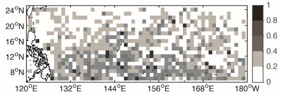
Figure 4.
The distribution of the probability of the BLT with thickness error less than 1% on 1 × 1 grids. Data used in the error calculation were collected from 2001 to 2010 during the TC-prevailing season.
There are in total 2295 validated profiles which were collected within the chosen grids (about 1.03 × 10⁶ km2 coverage) during TC-prevailing season from 2000 to 2010. The statistics reveal that BLT with 0–5 m occupies the highest proportion (Table 2). Some BLTs are negative, which can also be found in Figure 3a, indicating that the ILD is shallower than the MLD, and are referred to as compensated layer. However, the compensated layer is beyond the scope of this study, so no further discussions about the compensated layer will be provided. Although the proportion of unapparent BL (0–5 m) accounts for nearly 70%, the thicker BL (>5 m) still takes up about 25–30%. We take much more interest in the latter, since only the BL with enough thickness (>5 m) could resist the entrainment cooling effectively.
Table 2.
Statistical percentage of BLT in different intervals which was computed from the chosen HYCOM gridded daily data in TC-prevailing season during the period from 1996 to 2010.
Moreover, the life length of daily BL with different thicknesses is compiled with the same HYCOM/NCODA solutions, as shown in Figure 5. BLs are categorized into three groups based on thickness: 0–5 m, 5–30 m, and greater than 30 m. Life lengths of the BLT with 0–5 m are almost limited to 5 days, but the thicker BLs possess more probability to live longer than 10 days. This result is comparable to the conclusion of Katsura et al. [29], suggesting that the temporal scale of BLs in the subtropical Pacific is on average shorter than 10 days. BL can be formed due to several mechanisms, such as the tilting process of sea surface salinity (SSS) front, advection of fresher surface water, turbulent mesoscale eddies etc. Diverse processes result in different characteristic temporal scale of BLs, which makes us believe that forces responsible for density stratification in the MDR are various; whether all kinds of BLs are effective in resisting the cooling response remains an interesting topic.
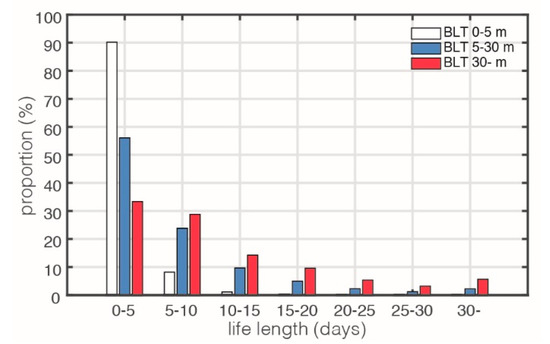
Figure 5.
Statistical proportion of the life length of BL with different thickness, which are 0–5 m (white bars), 5–30 m (blue bars), and over 30 m (red bars). The time range of the collected BL data is from 2001 to 2010.
To understand the spatial extent of BL, the coverage proportion (area occupied by the detected BLs with thickness ≥ 5 m relative to the total area of MDR) and the average thickness of daily BLs over 5 m in the recent decade (2001–2010) are displayed and analyzed using linear regression (Figure 6). The BL coverage proportion and thickness both increase with time, which indicates that stratification of the upper ocean layer is stabilizing. However, there is a discrepancy in thickness growth rate between each location since the standard deviation of average BLT (gray shading in Figure 6b) is also increasing. Coverage proportion of the chosen grids changes between 10% to 40% in 2001, and generally expands by almost 50% after ten years. In other words, TC–BL interactions can occur more frequently in the future if the increasing trend of BL remains unchanged. Besides, the impact of El Niño-Southern Oscillation (ENSO) on BLT interannual variability is also observed. Both the coverage and thickness of BL tend to increase in the La Niña periods (2007/2008/2010) and decrease in the El Niño periods (2002/2004/2009). Interannual variability of the BL is further discussed in the following section in detail.
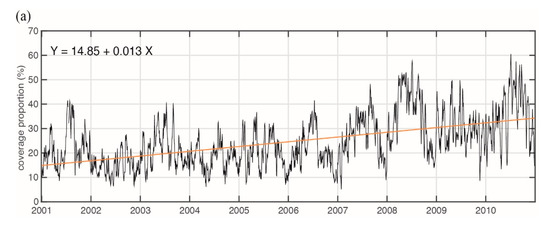
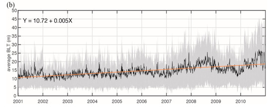
Figure 6.
Daily coverage proportion (a) and average thickness (b) with ± one standard deviation (gray shading) of mesoscale BL ≥ 5 m within the chosen grids. Time intervals are the TC-prevailing season in each year from 2001 to 2010. Orange lines indicate the first order linear regression lines of coverage and mean thickness.
3.3. Interannual Variability of BL
The empirical orthogonal function (EOF) analysis is applied to understand the longer-term temporal and spatial pattern of BLT in the MDR. The input data is monthly mean anomaly of BLT during TC-prevailing season (July–November), with seasonal variation filtered out (minus the climate average of 1961–2010). The sampling error of the significance of the modes are computed as , where is the given eigenvalue and N is the number of realizations (=250 in this case) [30]. Only the first and the second modes are conformed to the rule of thumb while determining the distinct eigenvalues. The first outcome spatial mode (Figure 7a) and time series of the principal component (PC) from the EOF analysis show that BLT in the MDR might have a strong relation to ENSO (Figure 7b). The Niño 4 index from Global Climate Observing System (GCOS), Earth System Research Laboratory (ESRL), is utilized for comparing the correlation between the first PC and ENSO. Although the variance explained by the first BLT mode is only 15.45%, its PC temporal pattern appears to correspond well with the time series of Niño 4 index (R = −0.69, satisfying the two-tailed t-test at 99% confidence level). The relation between BL and ENSO in low latitude (equatorial region) has been investigated comprehensively [11,31,32,33,34], and BL is considered as one of the key factors in establishing the warm pool migration and maintaining the heat buildup during ENSO events [35]. Nevertheless, the other regions (e.g., the MDR) are seldom discussed in the previous studies.
Figure 7.
(a) Main development region empirical orthogonal function (EOF) spatial pattern of the first BLT mode calculated with the TC-prevailing season (July–November) in the period of 1961–2010, and (b) time series of the principal component associated with the first BLT mode. (c) is the second BLT mode and (d) is the corresponding time series as well. Both of the principal components have been normalized. Black solid line in (b) is the Niño 4 index accessed from the Global Climate Observing System (GCOS) climate indices.
Based on the fact that the upper ocean density stratification results from the gradient of temperature and salinity (Tz and Sz), we employ the same EOF method in decomposing vertical temperature and salinity gradient, which are also computed from ORAS4 data. PCs of BLT are used to correlate with the PCs of temperature and salinity gradients at each depth above 200 m. The result shows that temperature and salinity gradients at 50 m depth mark the highest correlation coefficients with PC1 and PC2, respectively, of BLT separately (Figure 8), which are R = 0.66 and R = −0.53, both satisfying the two-tailed t-test at 99% confidence level. This information suggests that the principal variation of interannual BLT in the MDR from 1961 to 2010 was dominated by the change in temperature structure, and the secondary variation is controlled by salinity structure. The assumption can be further confirmed by the partial correlation analysis between the Tz, Sz, and BLT PC1 and PC2 (see Figure 9). It is found that the spatial patterns of area showing correlation are quite coincident with BLT mode 1 and mode 2 (Figure 7), and besides, the negative correlations between Tz and BLT PC1 as well as Sz and BLT PC2 (green shaded area in Figure 9) are the primary reasons for the positive phase in BLT mode 1 and mode 2 respectively. During the TC-prevailing seasons, the average temperature in the MDR decreases with depth (Tz > 0), but average salinity commonly increases with depth (Sz < 0). Variations of vertical gradient of temperature or salinity at the subsurface indirectly influence the ILD and MLD. Reduction of Tz (getting smaller but still positive) makes the threshold of ILD harder to reach, which deepens the ILD. As for the reduction of Sz (getting more negative), the water in the layer above changes faster and the MLD declines. Therefore, BLT expands when the magnitude of Tz decreases or the magnitude of Sz increases, and vice versa.
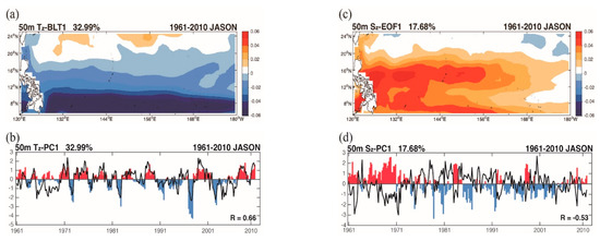
Figure 8.
(a) Main development region EOF spatial pattern of the first vertical temperature gradient (at 50 m depth) mode calculated with the TC-prevailing season (July–November) in the period of 1961–2010, and (b) time series of the PC associated with the first Tz mode. (c) is the same as (a), but represents the vertical salinity gradient instead. (d) is the corresponding time series of Sz mode as well. Both of the PCs have been normalized. Black solid lines in Figure 8b,d are the PC1 and PC2 from Figure 7.
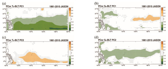
Figure 9.
Spatial distribution of the partial correlation coefficients between the Tz, Sz, and BLT PC1 (a) and (b). (c) and (d) are the same as (a) and (b), but are correlated with BLT PC2 instead. The matrix inversion method is applied to the partial correlation, and the input data are time series of Tz, Sz, and PC1 or PC2 on each grid (1 × 1) in the MDR. Color bar range of correlation coefficient is from −0.8 to 0.8 with an interval of 0.2. Dotted grids are the regions that the two-tailed t-test at 90% confidence level is satisfied.
Although the time series of the second BLT mode does not have a clear relation to prominent teleconnection patterns, its distribution of high variation area quite matches the location of the North Equatorial Current (NEC) and the north boundary of the North Equatorial Countercurrent (NECC). The NEC is part of the North Pacific subtropical gyre that flows westward, separating into northward flowing Kuroshio and southward flowing Mindanao Current at the Philippine coast. The NEC includes a zonal salinity front that separates the southern fresh NECC water from the northern saline subtropical water. Therefore, it is clear that the movement of NEC is important to the distribution of ocean salinity front in the MDR. The long-term change of the NEC bifurcation has been investigated previously [36,37], which claimed a quasi-decadal meridional migration of the NEC bifurcation between 10° N and 15° N.
Hence, the possible mechanism behind the first mode of BLT seems to be the well-known, zonal translation of thermal structure accompanying the ENSO; the second mode might be caused by the change of local salinity field, which could be induced by the precipitation anomaly (e.g., Philippine Sea Anomalous Anticyclone/Cyclone) [38,39], advected by the ocean current systems subsequently. Nevertheless, the vertical motion and the salinity change caused by the precipitation and evaporation at the air–sea interface should also be considered in the BL formation. The contributive ratio of the ocean horizontal motions to other terms of BL seasonal and interannual variability is an unsolved problem.
4. Conclusions and Remarks
In order to improve the tropical cyclone intensity forecasts, it is necessary to quantitatively evaluate the effect of TC–ocean interactions on tropical cyclone intensity. For quantitative evaluation of TC intensification rate and the maximum intensity, it is important to understand how the upper ocean structure varies depending on the upper ocean stratification and atmospheric forcing. In order to improve the TC intensity seasonal forecasts, it is important to understand the influence of interannual variations in the barrier layer on TC activity. In this study, a systematic statistical analysis is performed using in-situ Argo floats measurements, HYCOM/NCODA reanalysis outputs for the period 2001–2010, longer-term (1961–2010) variation of ORAS4 monthly BL, and JTWC TC data in the MDR to understand the characteristics of the BL in the WNP for different temporal scales and to quantify its capacity to resist TC induced sea surface cooling and thus the consequential possible TC enhancement. First, in addition to BL, a warm subsurface layer, low wind speed, and high translational speed are also considered as favorable conditions for minimal surface cooling after the TC passage, and these expected relations were reproduced by the statistical analysis. However, the relation between BLT and ΔT is not as clear as the with other factors, especially for the TC cases. Further analysis using partial correlation showed that the BL plays a role in resisting the cooling response only while the BL is strong enough (BLT ≥ 5 m) and/or TC wind forcing is not that strong. This result is consistent with the findings from a recent model study [27] that the effect of BL on TC intensification is depended on the depth where TC forcing can actually break through.
To examine the mesoscale characteristic of BL within the MDR in the WNP, BL is further analyzed for its distribution based on its thickness and life length. BLT with 0–5 m occupies the highest proportion (~67.55%). Thicker BL (BLT greater than 5 m) takes up about 25–30%. Also, there are ~3% BL with thickness greater than 30 m. As for life length, BLT with 0–5 m is almost limited to 5 days, while BLs with a thickness more than 30 m can persist to more than 30 days. Overall, the thicker BLs possess more probability to live longer than 10 days. This result is attributed to diverse processes responsible for different characteristic/temporal scales of BL, such as tilting process of SSS front, advection of fresher surface water, and turbulent mesoscale eddies etc. Analysis of the BL coverage portion and average BLT in the recent decade showed a sharp increase in both the spatial coverage and thickness of BL. This implies that the impact of BL on TC enhancement can occur more frequently and vigorously, which is a serious scenario that predicts the occurrences of stronger TCs in the MDR in the near future.
Finally, the empirical orthogonal function (EOF) analysis is applied to provide the detailed information about the longer-term interannual variability of BLT in the MDR in the past 50 years (1961–2010). Dominant modes show that the interannual variability of BLT in the MDR might be influenced by the ENSO and migration of NEC. Additionally, given the fact that the upper ocean density stratification results mainly from the gradient of temperature and salinity (Tz and Sz), long-term interannual variability of vertical temperature and salinity gradient are also decomposed by EOF analysis. The cross EOFs comparison shows that the principal variation of interannual BLT in the MDR (EOF mode 1) is dominated by the change of temperature structure, and salinity structure plays the secondary role. A detailed discussion on the progress of temperature and salinity structures leading to the variability of long-term interannual BLT is given separately in Section 3.3. The key mechanism leading to the interannual variability of 2nd mode of BLT is attributed to the local ocean salinity front advected by the migration of NEC.
Studies about factors related to TC development and enhancement are important and beneficial for improving the accuracy of TC intensity forecasts. The results shown in this study not only provide one step toward more understanding about the characteristics of BL in different temporal scales but also point out the increasingly important role played by BL in the MDR in the WNP with statistical evidences. However, a comprehensive understanding about how the BL resisting TC induces upper ocean responses (including both thermal, saline, and other possible paths) requires further investigation.
Author Contributions
D.-R.W., G.G. and Z.-W.Z. conceived and designed the study. G.G. contributed to English editing. C.-R.H. and Q.Z. contributed to the writing and data interpretation. Data analyses were conducted mainly by D.-R.W. All authors have read and agreed to the published version of the manuscript.
Funding
This research was funded by Taiwan’s Ministry of Science and Technology (MOST) under 108-2628-M-003-001-MY3.
Institutional Review Board Statement
Not applicable.
Informed Consent Statement
Not applicable.
Data Availability Statement
Not applicable.
Acknowledgments
The authors would like to thank the anonymous reviewers for their very constructive comments. Thanks to JTWC, ECMWF, Argo, HYCOM scientific teams for providing the essential data sets.
Conflicts of Interest
The authors declare no conflict of interest.
References
- Leipper, D.F.; Volgenau, D. Hurricane Heat Potential of the Gulf of Mexico. J. Phys. Oceanogr. 1972, 2, 218–224. [Google Scholar] [CrossRef]
- Palmen, E. On the formation and structure of tropical cyclones. Geophyisca 1948, 3, 26–38. [Google Scholar]
- Perlroth, I. Effects of oceanographic media on Equatorial Atlantic hurricanes. Tellus 1969, 21, 230–244. [Google Scholar] [CrossRef]
- Shay, L.K.; Brewster, J.K. Oceanic Heat Content Variability in the Eastern Pacific Ocean for Hurricane Intensity Forecasting. Mon. Weather. Rev. 2010, 138, 2110–2131. [Google Scholar] [CrossRef]
- Shay, L.K. Air-Sea Interactions in Tropical Cyclones. In Global Perspectives on Tropical Cyclones: From Science to Mitigation; Johnny, C.L.C., Jeffrey, D.K., Eds.; World Scientific Publishing Co. Pte. Ltd.: Singapore, 2010; Volume 4, pp. 93–132. [Google Scholar]
- Emanuel, K.A. Thermodynamic control of hurricane intensity. Nat. Cell Biol. 1999, 401, 665–669. [Google Scholar] [CrossRef]
- Price, J.F. Upper ocean response to a hurricane. J. Phys. Oceanogr. 1981, 11, 153–175. [Google Scholar] [CrossRef]
- Balaguru, K.; Chang, P.; Saravanan, R.; Leung, L.R.; Xu, Z.; Li, M.; Hsieh, J.-S. Ocean barrier layers’ effect on tropical cyclone intensification. Proc. Natl. Acad. Sci. USA 2012, 109, 14343–14347. [Google Scholar] [CrossRef]
- Lin, I.I.; Wu, C.-C.; Emanuel, K.A.; Lee, I.-H.; Wu, C.-R.; Pun, I.-F. The Interaction of Supertyphoon Maemi (2003) with a Warm Ocean Eddy. Mon. Weather. Rev. 2005, 133, 2635–2649. [Google Scholar] [CrossRef]
- Wu, C.-C.; Lee, C.-Y.; Lin, I.-I. The Effect of the Ocean Eddy on Tropical Cyclone Intensity. J. Atmos. Sci. 2007, 64, 3562–3578. [Google Scholar] [CrossRef]
- Sprintall, J.; Tomczak, M. Evidence of the barrier layer in the surface layer of the tropics. J. Geophys. Res. Space Phys. 1992, 97, 7305–7316. [Google Scholar] [CrossRef]
- Cronin, M.F.; McPhaden, M.J. Barrier layer formation during westerly wind bursts. J. Geophys. Res. Space Phys. 2002, 107. [Google Scholar] [CrossRef]
- Peduzzi, P.; Chatenoux, B.; Dao, Q.-H.; De Bono, A.; Herold, C.; Kossin, J.; Mouton, F.; Nordbeck, O. Global trends in tropical cyclone risk. Nat. Clim. Chang. 2012, 2, 289–294. [Google Scholar] [CrossRef]
- Mignot, J.; Montégut, C.D.B.; Tomczak, M. On the porosity of barrier layers. Ocean Sci. 2009, 5, 379–387. [Google Scholar] [CrossRef]
- Sato, K.; Suga, T.; Hanawa, K. Barrier layers in the subtropical gyres of the world’s oceans. Geophys. Res. Lett. 2006, 33. [Google Scholar] [CrossRef]
- Balmaseda, M.A.; Mogensen, K.; Weaver, A.T. Evaluation of the ECMWF ocean reanalysis system ORAS4. Q. J. R. Meteorol. Soc. 2013, 139, 1132–1161. [Google Scholar] [CrossRef]
- Gould, J. From swallow floats to Argo-The development of neutrally buoyant floats. Deep Sea Res. Part II 2005, 52, 529–543. [Google Scholar] [CrossRef]
- Cummings, J.A. Operational multivariate ocean data assimilation. Q. J. R. Meteorol. Soc. 2005, 131, 3583–3604. [Google Scholar] [CrossRef]
- Akima, H. A New Method of Interpolation and Smooth Curve Fitting Based on Local Procedures. J. ACM 1970, 17, 589–602. [Google Scholar] [CrossRef]
- Greatbatch, R.J. On the Response of the Ocean to a Moving Storm: The Nonlinear Dynamics. J. Phys. Oceanogr. 1983, 13, 357–367. [Google Scholar] [CrossRef]
- Lloyd, I.D.; Vecchi, G.A. Observational evidence for oceanic controls on hurricane intensity. J. Clim. 2011, 24, 1138–1153. [Google Scholar] [CrossRef]
- Gill, A.E. Atmosphere-Ocean Dynamics; Appendix 3; Academic Press, Inc.: New York, NY, USA, 1982; pp. 599–600. [Google Scholar]
- Geisler, J.E. Linear theory of the response of a two layer ocean to a moving hurricane. Geophys. Fluid Dyn. 1970, 1, 249–272. [Google Scholar] [CrossRef]
- Chang, Y.-C.; Chen, G.-Y.; Tseng, R.-S.; Centurioni, L.R.; Chu, P.C. Observed near-surface flows under all tropical cyclone intensity levels using drifters in the northwestern Pacific. J. Geophys. Res. Oceans 2013, 118, 2367–2377. [Google Scholar] [CrossRef]
- GirishKumar, M.S.; Ravichandran, M.; McPhaden, M.J. Temperature inversions and their influence on the mixed layer heat budget during the winters of 2006-2007 and 2007-2008 in the Bay of Bengal. J. Geophys. Res. Oceans 2013, 118, 2426–2437. [Google Scholar] [CrossRef]
- Mignot, J.; Lazar, A.N.; Lacarra, M. On the formation of barrier layers and associated vertical temperature inversions: A focus on the northwestern tropical Atlantic. J. Geophys. Res. Space Phys. 2012, 117, 02010. [Google Scholar] [CrossRef]
- Yan, Y.; Li, L.; Wang, C. The effects of oceanic barrier layer on the upper ocean response to tropical cyclones. J. Geophys. Res. Oceans 2017, 122, 4829–4844. [Google Scholar] [CrossRef]
- Rudzin, J.E.; Shay, L.K.; Johns, W.E. The Influence of the Barrier Layer on SST Response during Tropical Cyclone Wind Forcing Using Idealized Experiments. J. Phys. Oceanogr. 2018, 48, 1471–1478. [Google Scholar] [CrossRef]
- Katsura, S.; Oka, E.; Sato, K. Formation Mechanism of Barrier Layer in the Subtropical Pacific. J. Phys. Oceanogr. 2015, 45, 2790–2805. [Google Scholar] [CrossRef]
- North, G.R.; Bell, T.L.; Cahalan, R.F.; Moeng, F.J. Sampling errors in the estimation of empirical orthogonal functions. Mon. Wea. Rev. 1982, 110, 699–706. [Google Scholar] [CrossRef]
- Bosc, C.; Delcroix, T.; Maes, C. Barrier layer variability in the western Pacific warm pool from 2000 to 2007. J. Geophys. Res. Space Phys. 2009, 114, 06023. [Google Scholar] [CrossRef]
- Soloviev, A.; Lukas, R. Observation of Spatial Variability of Diurnal Thermocline and Rain-Formed Halocline in the Western Pacific Warm Pool. J. Phys. Oceanogr. 1996, 26, 2529–2538. [Google Scholar] [CrossRef]
- Wang, X.; Liu, H. Seasonal-to-interannual variability of the barrier layer in the western Pacific warm pool associated with ENSO. Clim. Dyn. 2016, 47, 375–392. [Google Scholar] [CrossRef]
- Qu, T.; Song, Y.T.; Maes, C. Sea surface salinity and barrier layer variability in the equatorial Pacific as seen from Aquarius and Argo. J. Geophys. Res. Oceans 2014, 119, 15–29. [Google Scholar] [CrossRef]
- Maes, C.; Picaut, J.; Kuroda, Y.; Ando, K. Characteristics of the convergence zone at the eastern edge of the Pacific warm pool. Geophys. Res. Lett. 2004, 31. [Google Scholar] [CrossRef]
- Chen, Z.; Wu, L. Long-term change of the Pacific North Equatorial Current bifurcation in SODA. J. Geophys. Res. Space Phys. 2012, 117, 06016. [Google Scholar] [CrossRef]
- Qiu, B.; Chen, S. Interannual-to-Decadal Variability in the Bifurcation of the North Equatorial Current off the Philippines. J. Phys. Oceanogr. 2010, 40, 2525–2538. [Google Scholar] [CrossRef]
- Wang, B.; Wu, R.; Fu, X. Pacific–East Asian Teleconnection: How Does ENSO Affect East Asian Climate? J. Clim. 2000, 13, 1517–1536. [Google Scholar] [CrossRef]
- Yuan, Y.; Yang, S. Impacts of Different Types of El Niño on the East Asian Climate: Focus on ENSO Cycles. J. Clim. 2012, 25, 7702–7722. [Google Scholar] [CrossRef]
Publisher’s Note: MDPI stays neutral with regard to jurisdictional claims in published maps and institutional affiliations. |
© 2021 by the authors. Licensee MDPI, Basel, Switzerland. This article is an open access article distributed under the terms and conditions of the Creative Commons Attribution (CC BY) license (http://creativecommons.org/licenses/by/4.0/).