1. Introduction
The growing auto-dependency in the United States (US) has been associated with many urban problems such as urban sprawl, pollutions, traffic congestions, and accidents. This means that as the use of private automobiles increases, transportation negative externalities also increase. Therefore, many cities in the US have built modern rail transit systems to mitigate the negative impact of higher dependency on automobiles and improve mobility and accessibility for commuters, offer an alternative to drivers, shape development patterns, and increase economic growth [
1,
2,
3]. The dependence on rail transit systems causes apparent shifts in neighborhoods’ economic, social, and spatial aspects close to rail stations [
3,
4]. This shift’s magnitude differs from city to city, even from different stations on the same line [
1]. Rail transit systems have wide-ranging impacts on development patterns and quality of life, and they can enhance economic growth [
5] and lead to agglomeration economies in some industries [
6]. These industries contribute to increased population and employment densities in the area surrounding rail stations [
6]. In addition, one of the major effects generated by rail transit systems is the positive changes in property value and rent [
7] due to better accessibility generated by rail transit systems [
8,
9].
However, rail transit stations might negatively affect station areas and decrease property value and population density. This is because of negative externalities associated with rail transit systems, such as higher traffic congestion, crime rates, noise, and pollution [
10,
11]. A zero or weak impact from rail transit systems is also reported in several studies regarding property value, rent, population densities, or changes in residents’ socioeconomic characteristics [
12].
This research examines if the effects of rail transit stations in the Dallas-Fort Worth (DFW) metropolitan area on nearby neighborhoods are positive, negative, or have no impact at all. The major impact taken into account is related to population density changes in some chosen geographic census units. These indicators can be analyzed in order to explore the impacts of proximity to rail transit stations on identified geographic census units within a certain distance from the rail stations.
2. Statement of the Problem and the Significance of Research
As mentioned in the introduction section, rail transit systems can affect rail stations’ population density either positively or negatively. Thus, planners believe that as the interest in building rail transit system increases, the need to understand the general impacts increases and becomes essential [
3]. Therefore, researchers should examine the changes in areas surrounding rail stations and compare the impacts over the last few years to the effects from a couple of years ago to understand and measure impact trends.
This research attempts to study the effects of the rail transit stations on the surrounding areas in the DFW metropolitan area and looks for population density changes over a long time to find and examine the extent and type of impacts resulting from proximity to rail transit stations. One of the strong reasons for this study in this specific metropolitan area is that there are very few published studies on rail transit in the DFW area. No analysis is found covering all of the region’s rail transit systems even though it has the most extensive rail transit network in the US [
13,
14]. Those few studies covered only Dallas Area Rapid Transit (DART) but not the entire system. However, there are many studies about the impact of rail transit systems in other major US cities. This situation prompts a need for this research. Moreover, the larger geographic area of the rail transit system may show better or different results than what other scholars have found in smaller study areas. Furthermore, cities served by rail transit in the DFW metropolitan area have a low population density, and they are auto-oriented cities. Therefore, the investment of rail transit in these cities may not improve the accessibility of a location enough to attract more residents and businesses to locate in proximity to rail stations, which makes the results of this study different from anywhere else.
As a result, this study is an addition to the literature related to urban planning in general. Specifically, it contributes valuable information to the literature associated with the impact of rail transit stations on the changes to the population density of neighborhoods surrounding rail stations—especially if those neighborhoods are located in a metropolitan area characterized by auto-oriented and low-density developments. The results of this study show that the rail transit stations affect population density; those factors are statistically significant and have strong relationships, and have major planning and policy implications on the affordability of housing and equitable mixed-use developments. Moreover, these planning and policy implications could be applicable to other large metropolitan areas. The study’s findings show some unexpected results related to the impacts of proximity to rail stations on population density changes. The findings could help urban planners and decision-makers adopt some local and government policies to motivate more sustainable development around rail stations to improve transit accessibility.
3. Review of the Literature
Even though there are very few studies about the impact of rail stations on population density as opposed to the effects on housing value, this section discusses relevant theories and existing studies. The theoretical basis for monocentric population density is derived from Von Thünen’s (1863) bid rent theory, which was subsequently developed by many other scholars, where the city center is valuable for some land uses since it is traditionally the most accessible location for a large population. This theory can be applied to rail transit stations since stations may also play the city center’s role [
4,
15]. Thus, rail transit systems’ improvement of transportation accessibility attracts developments and commercial activities, raising property value near rail stations, thereby causing a higher population density since landowners want to offset the higher land value [
16].
Since many local authorities in North America regain momentum in using transit rail, many planners have begun to think about guiding development toward rail transit areas. It is believed that it would restrict metropolitan areas from more sprawl and car dependency, inducing higher density development [
17]. Therefore, some cities have adopted higher development densities around stations; others saw transit stations as nodes for offices and retail activities. Still, other cities applied transit-oriented development (TOD) in areas surrounding stations [
17]. However, in many cases, urban growth does not follow the transit systems, and the impact of rail stations on development patterns is not as direct as many planners expect [
17].
Many studies confirm that rail transit systems increase the surrounding neighborhoods’ population density, but others do not. Badoe and Miller [
18] found that not only did areas closer to rail transit stations experience greater population density, but all parts of Philadelphia experienced either an equal or greater increase. Bernick and Cervero [
19] mentioned that approximately 12,000 multifamily units were built around rail stations within 10 major metropolitan areas between 1988 and 1993. A study by Shen [
20] showed that most of the station areas were associated with higher population and housing densities for four major metropolitan regions, Chicago, Denver, Los Angeles, and Washington, DC, between 1990 and 2010. Another study by Arrington and Cervero [
21] examined the residential density changes around 17 rail stations in four urbanized areas and found that residential density increased by 20% to 330%. Hurst and West [
16] found that multifamily housing increased by 11.3% in neighborhoods surrounding METRO Blue stations in Minneapolis during the construction, and 16.6% after opening the rail system.
However, rail transit systems can generate negative externalities that can harm population density [
22,
23]. Moreover, several studies found that many commercial uses over time tended to replace residential and industrial uses in proximity to stations [
24]. For example, Dueker and Bianco [
25] surveyed the Eastside MAX rail line’s effect in Portland, OR, on residential density between 1986 and 1995. The results showed that the net residential density declined in both the areas surrounding rail stations by 1.60% due to a significant increase in commercial uses within block groups covering rail stations.
Bollinger and Ihlanfeldt [
26] estimated the Metropolitan Atlanta Rapid Transit Authority (MARTA) impact on the population’s densification surrounding station areas. They found the mean change in population was considerably greater in non-station areas than in station areas. In addition, another study found that census tracts around MARTA stations lost 11% of their residents, whereas employment increased by 13% [
27]. In the study conducted by Farrow [
28] about land use patterns around 20 DART stations, the most significant change was around northern stations, where many commercial and multifamily housing units existed; many single-family residential housing subdivisions were constructed near the southern stations.
The magnitude of the impact can vary based on neighborhood and spatial contexts. For instance, investments in rail transit systems in lower density or auto-oriented cities, such as Minneapolis and Dallas, might not attract more population and investments to relocate in close proximity to rail stations [
29,
30].
As mentioned before, some studies found a strong relationship between rail transit stations and population density. Still, this population density did not necessarily result solely from the proximity to the rail stations [
31]. Some noted that population density might increase due to proximity to highway ramps [
32]. Furthermore, population density might have been affected positively or negatively by some land uses [
24]. For example, it was affected negatively by the manufacturing sector [
32], landfills, waste sites, and industrial facilities [
33] but was affected positively by the service and retail trade sectors [
32]. Most of the transit stations developed as TODs represent mixed-use developments with moderate to high density [
34]. There is a direct proportion between the number of amenities increases in a neighborhood and land demand. The result is a higher land value [
35] and therefore increasing population density [
36].
The results of the preceding studies that surveyed the changes in population density next to rail stations were mixed and inconsistent; results were different from one research to another in presence, magnitude, and range of the impact on population density changes. In some of them, transit areas experienced higher population density. Other cases found that neighborhoods surrounding rail stations experienced a decline in population density after operating the rail transit system and were more attractive to commercial uses. Moreover, some of the existing studies concluded that proximity to rail stations did not affect population density in any way. Furthermore, some of the prior research found an increase in population density with some stations and decreased with others within the same transit system. Most previous studies have been conducted in US cities with similar urban features to the current study location. Almost all of them are auto-dependent, low-density communities that stimulate sprawl patterns, while the higher population density is increased with proximity to central business districts (CBDs).
4. The Geographical Limitation
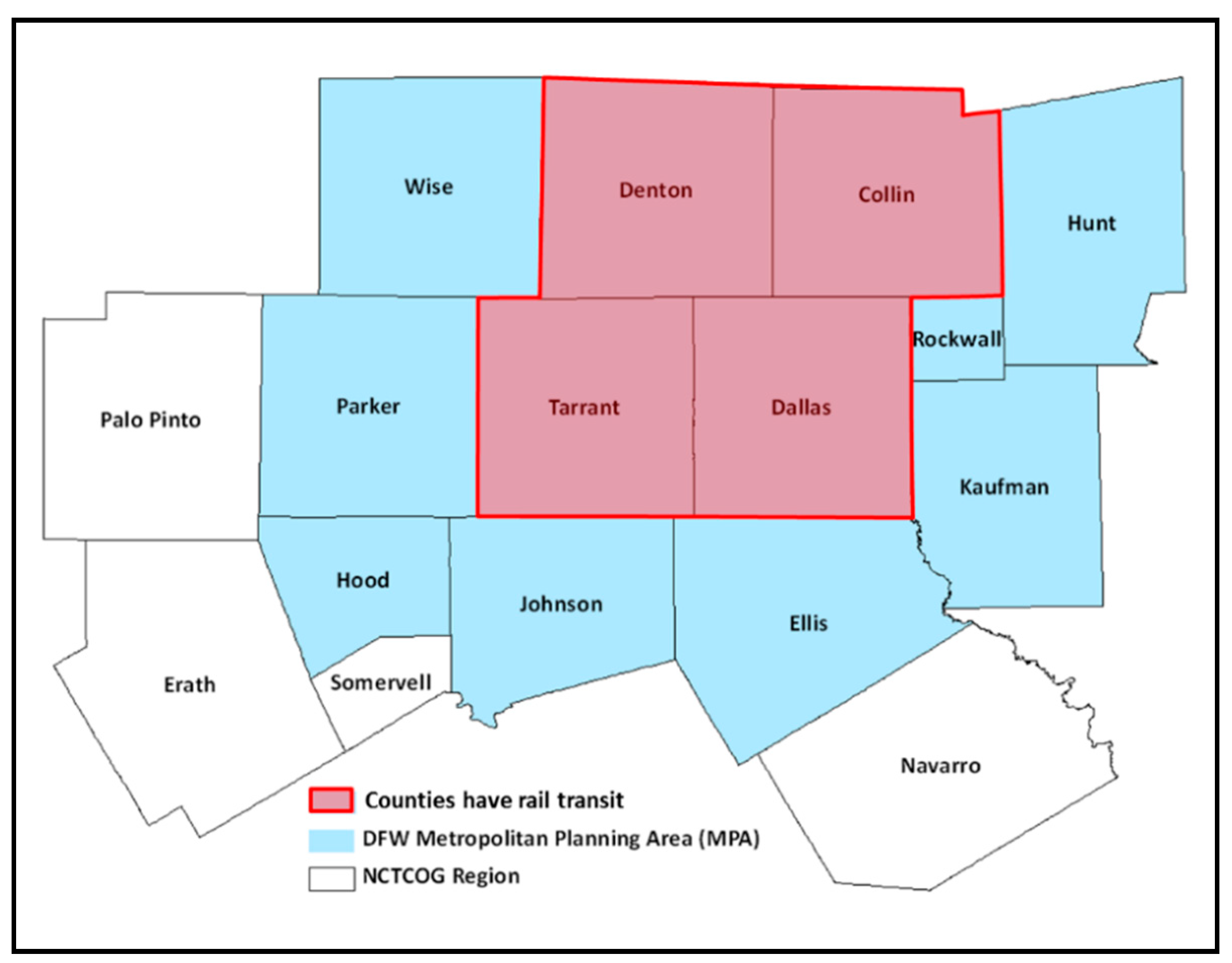
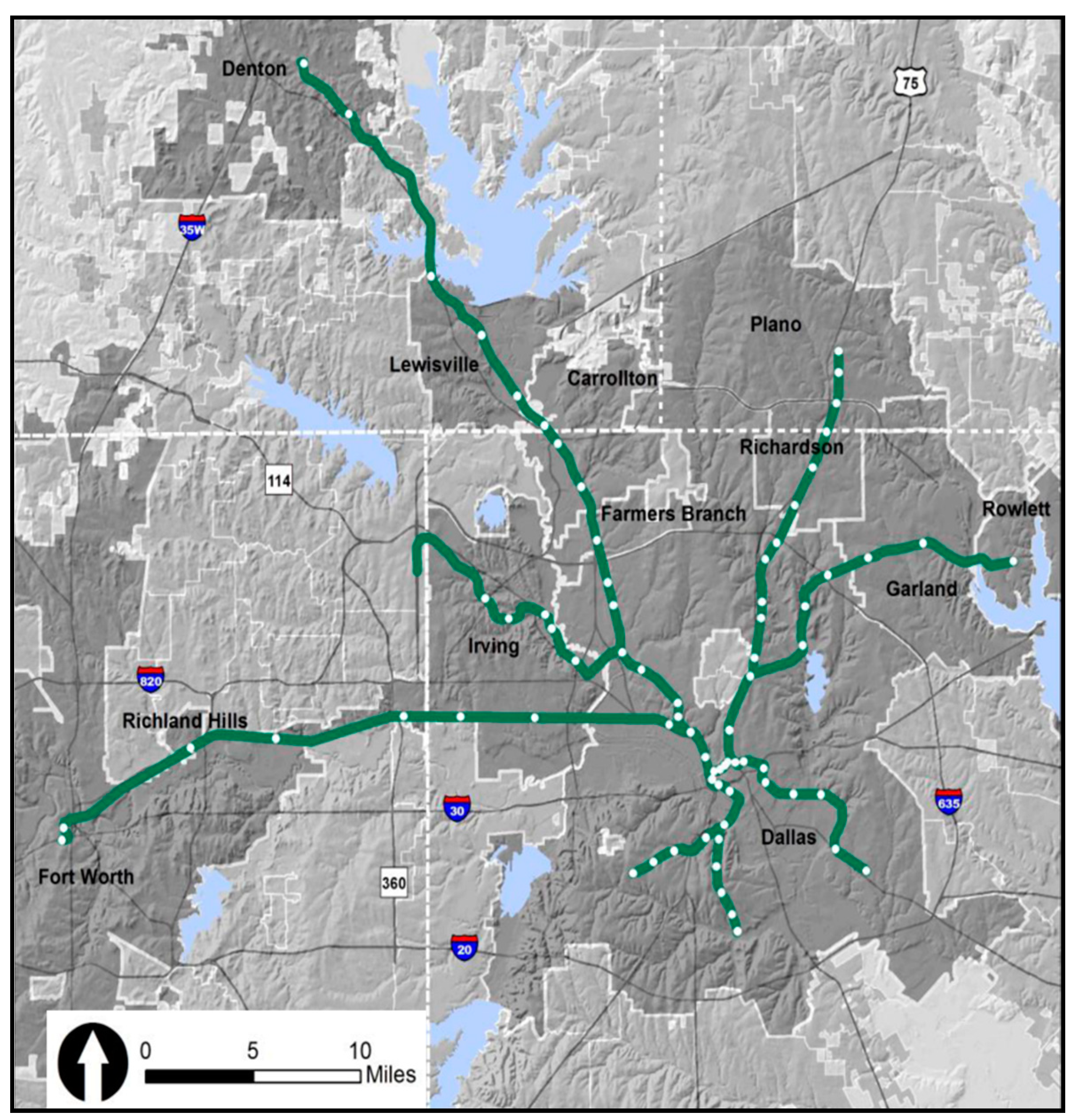
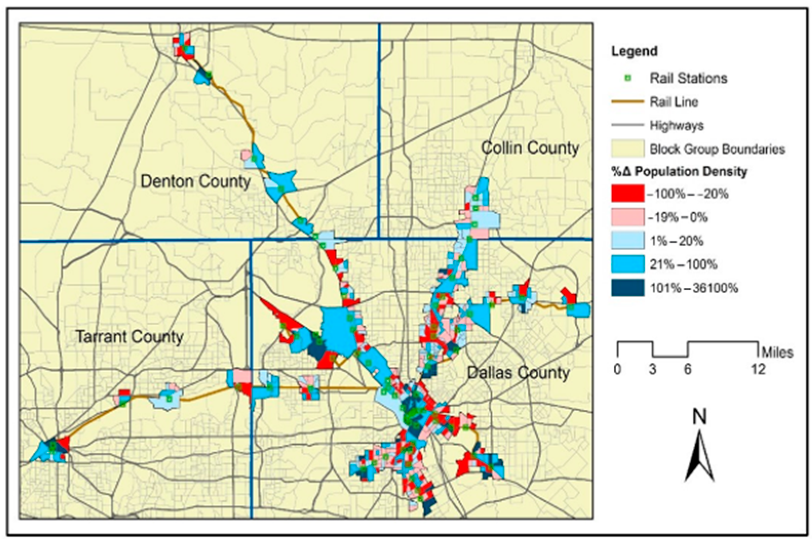
This study covers rail passenger transportation in the DFW metropolitan area that serves four urban counties (Collin, Dallas, Denton, and Tarrant) (
Figure 1). In total, 74 transit rail stations serve 20 cities in this area along 146 miles of light and commuter rail (
Figure 2). Furthermore, 32 rail transit stations in this rail system are reasonably developed as TODs, whereas 42 stations can be considered non-TODs [
29].
5. Methods and Techniques
After reviewing the existing literature about rail stations’ impact on the neighboring areas, a solid theory has not been found to guide scholars in deciding the range of proximity affected by rail transit facilities [
20]. The impact of rail stations usually falls within a limited distance, and this distance is mainly determined by the feasible distance for walking to and from the rail stations. The shortest and dominant proximity measure found in the literature is one-quarter mile from stations. However, in practice, a one-quarter mile radius may not capture all rail transit impacts since some effects may extend farther out. Accordingly, one-half mile can be the distance that transit riders can walk to and from rail stations, and many prior studies have used a one-half mile buffer around stations. However, other scholars challenged the traditional one-half mile standard measure and argued that transit riders were able to walk one mile or even more. This is because people in average physical condition can walk this distance in around 15 to 17 min, which is a reasonable time to reach a station [
37,
38,
39,
40]. Moreover, more people will dive to transit stations if a park-and-ride facility is available. This will definitely increase the rail transit influence [
33,
36,
37,
38]. Some of the existing studies found that a two-mile radius is statistically significant and can adequately capture the impact of transit stations [
41,
42]. Moreover, block groups outside of major downtowns are large, and choosing a smaller radius would result in very few block groups being captured within the study area [
43].
Additionally, many studies included multiple rings around stations ranging from two to five rings. Those rings are usually divided into one-quarter or one-half mile segments. For example, Bowes and Ihlanfeldt [
44] found that the impact of MARTA stations in Atlanta affected residential and commercial properties up to three miles from rail stations. Still, the significant impact occurred within the first half a mile from stations. Moreover, Pan [
45] found that the Houston METRORail stations’ impact on home prices extended three miles from stations. A couple of existing studies did not identify any positive or negative impact within the first ring but found some effect in subsequent rings due to negative externalities associated with rail transit systems [
44,
46,
47,
48]. Thus, this study will use a one-mile buffer around rail transit stations due to the reasons discussed above.
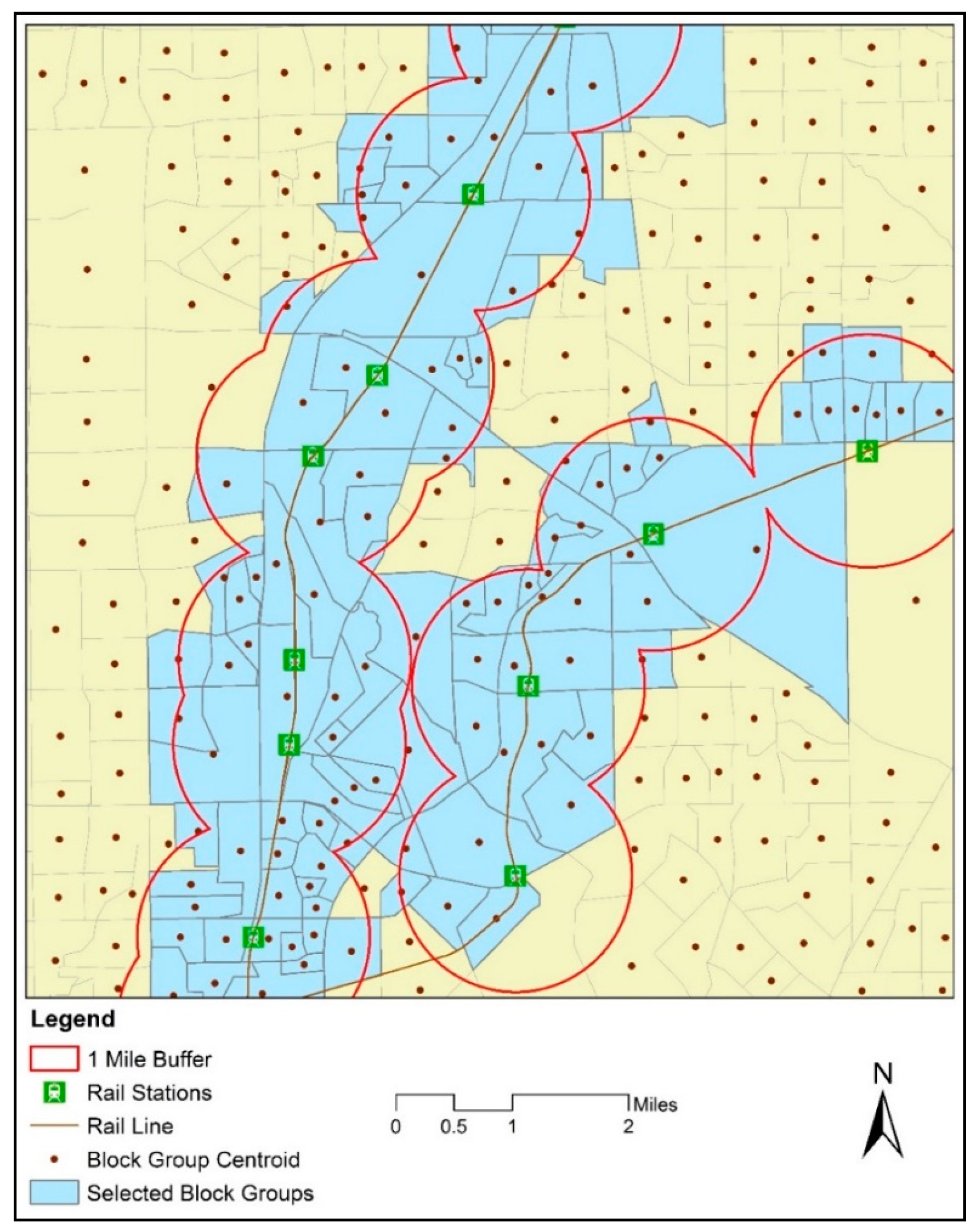
The centroid containment method is used when we select the block groups for this study. This study’s chosen block groups should have either half or more than half of their area within the buffer, or their centroid points lie within the buffer (
Figure 3). This method is chosen since it is more accurate than other selection methods [
44]. The straight-line distance method is used to measure the accessibility distance from transit stations. Most previous studies also used this method and did not find significant differences in the network distance. Furthermore, some authors [
29,
49,
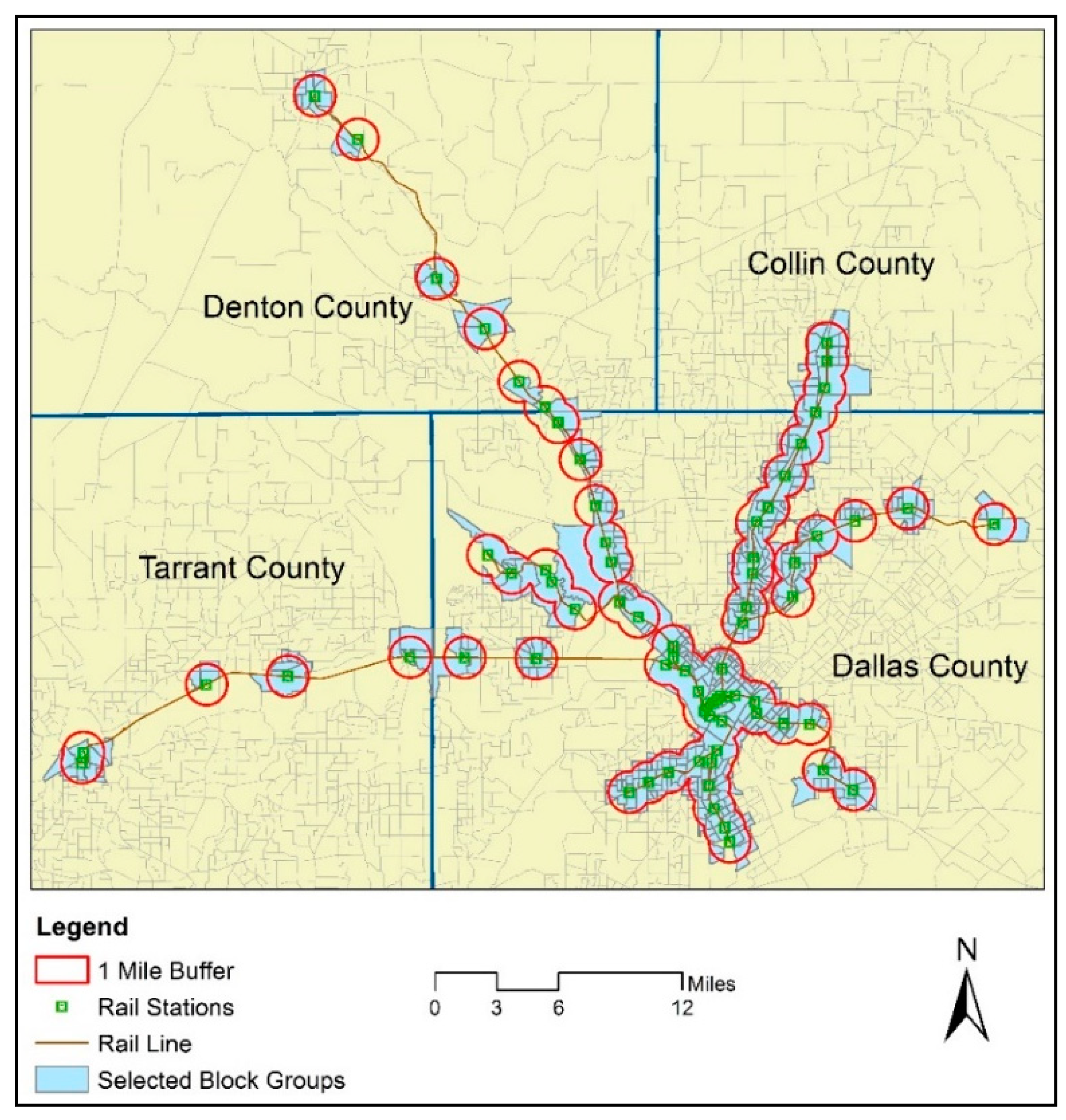
50] have tested this technique and found it statistically significant. The number of block groups that satisfy the selected criterion and are used in this study is 454, see
Figure 4.
6. Spatial Analysis and Statistical Tests
In this study, we use three approaches. Firstly, to compare population density changes within selected block groups between 2000 and 2014, the before-and-after method is used. Secondly, the matched-pair analysis is used to compare the study area to the rest of the block groups of the “non-station areas” located within the four counties served by the rail transit system between 2000 and 2014. Finally, these approaches are followed by a multiple regression model that is used to reject the null hypothesis and answer the research question.
To understand better the impact of the rail transit stations on residents’ population density around and far from it over time, the percentage change is used. This allows the comparison between population densities at different times.
The Kruskal–Wallis test, known as one-way ANOVA [
51], was conducted to examine whether or not the variations among all percentage changes of variables between 2000 and 2014 in the study area’s non-station areas are statistically significant.
As was mentioned, the third stage used multiple regression models to analyze the change in population density (ΔPopDen) as the dependent variable for each block group within the study area. The independent variables are obtained from theories and literature reviews that show how rail transit stations have led to population density changes. They can be categorized based on the control variables that can affect population density. These including proximity to transportation access variables, proximity to other land use variables, proximity to amenities and disamenities variables, demographic composition variables, land value variables, and employment density variables.
The first category of control variables affecting population density next to rail transit stations is transportation accessibility. Clark primarily developed the density gradient concept in 1951, in which he found that population density falls within distance from the city center. Based on bid rent theory, the city center is valuable for some land uses because it is traditionally the most accessible location for a large population. Consequently, land prices are higher in proximity to the CBD—the farther the distance from the CBD, the cheaper the land. This is why city downtown areas are densely populated, while suburbs and rural areas are more sparsely populated, with detached houses and low-density [
31]. The bid rent model can be applied to rail transit stations since stations may play the role of the center of the city [
4,
9]; the higher land value next to stations causes changes in development patterns and growth in population density (unless there are zoning or other restrictions). Weinberger [
52] pointed out that higher land prices in proximity to rail stations led to more densely developed areas since landowners want to offset the higher land value. Moreover, housing demand increases since many people wish to benefit from reducing commuting costs and better accessibility. Users of highways may benefit from increased accessibility associated with a decrease in commuting cost and time; non-users such as individuals and firms may also benefit from them in indirect ways [
26]. The increased accessibility results from highways attract more residents and produce a greater density in the nearby areas [
26].
Although proximity to the CBD, rail stations, or highway ramps can be considered as factors affecting population density functions, some authors have also found other factors to explain population density functions. According to Baumont et al. [
53], there is interdependence between employment and population suburbanization. Furthermore, the central city’s industrial uses were among the major forces behind residential suburbanization because of negative externalities that affected residents adversely. At the same time, retail employment density had a positive and significant relationship with population density [
32]. Moreover, Palm et al. [
54] showed that the most important determinants of population density were housing prices and neighborhood quality. Some other land uses can negatively affect residential land value and density, such as landfills, waste sites, nuclear power plants, hazardous manufacturing facilities, and industrial facilities [
32,
33].
Regarding different land uses next to rail stations, Schuetz [
55] argued that denser neighborhoods surrounding rail stations were positively associated with commercial land uses since these neighborhoods can provide more consumers. In short, commercial, service, and retail land uses may generate higher population density due to the high demand between residents and firms selling goods to consumers. Reduced vacant land may increase the number of residents in these areas, but landfills, waste sites, and industrial uses are adversely associated with population density.
Most of the transit stations developed as TODs represent mixed-use development with moderate to high density. They are designed to encourage people to bike and walk in the area adjacent to rail stations. In addition, as the number of amenities increases in a neighborhood, the demand for lands increases, resulting in a higher residential value [
35], which causes changes in development patterns and increases population density [
36].
Based on bid rent theory, property with proximity to the city’s center has a higher price than more distant properties [
36]. Landowners are willing to offset the higher cost of land in the CBD and maximize the property returns [
17]. Therefore, some land will be converted to higher-density uses, such as multifamily housing units, retail, and offices. Hence, the CBD is expected to grow and develop [
17]. Changes in some demographic compositions over time may affect the shape of the population density gradient. Smith [
56] noted that during the 1960s and 1970s, several researchers found changes in the population density gradient because of certain historical, spatial, and socioeconomic factors. For instance, higher-income households preferred single-family housing with a large lot size, resulting in lower population density. In addition, Mills [
57] used a two-point method and found that the major determinants of historical leveling out of the population density function were population size and income. Alperovich [
58] added that as income increased, the demand increased for high-quality and low-density neighborhood housing. He also stated that as the households’ incomes increased, they would shift their bids for housing away from the city center, where the quality of housing and neighborhood were low, and density was higher, to areas farther away, where the quality of housing and neighborhood were higher, and density was low. This shift resulted in changes in population density in proximity to the CBD and suburbs—since the increase in income caused a flattening in density gradients. As stated earlier, most of the independent variables that may affect population density are considered, as shown in
Table 1. Therefore, the regression function is as follows:
Table 1 below presents the four categories with all explanatory variables behind each category, along with definition and the sign of their expected impact on the median change in population desnity. Here, a positive (+) sign indicates that it is expected to have positive relationship with the dependent variable. A negative sign (−) means a hypothesized negative relationship between the dependent and independent variable, and (?) means uncertain relationship.
7. Descriptive Analysis
Data from various sources are collected and joined. The four counties’ selected block groups are then extracted from the rest of the block groups for analysis.
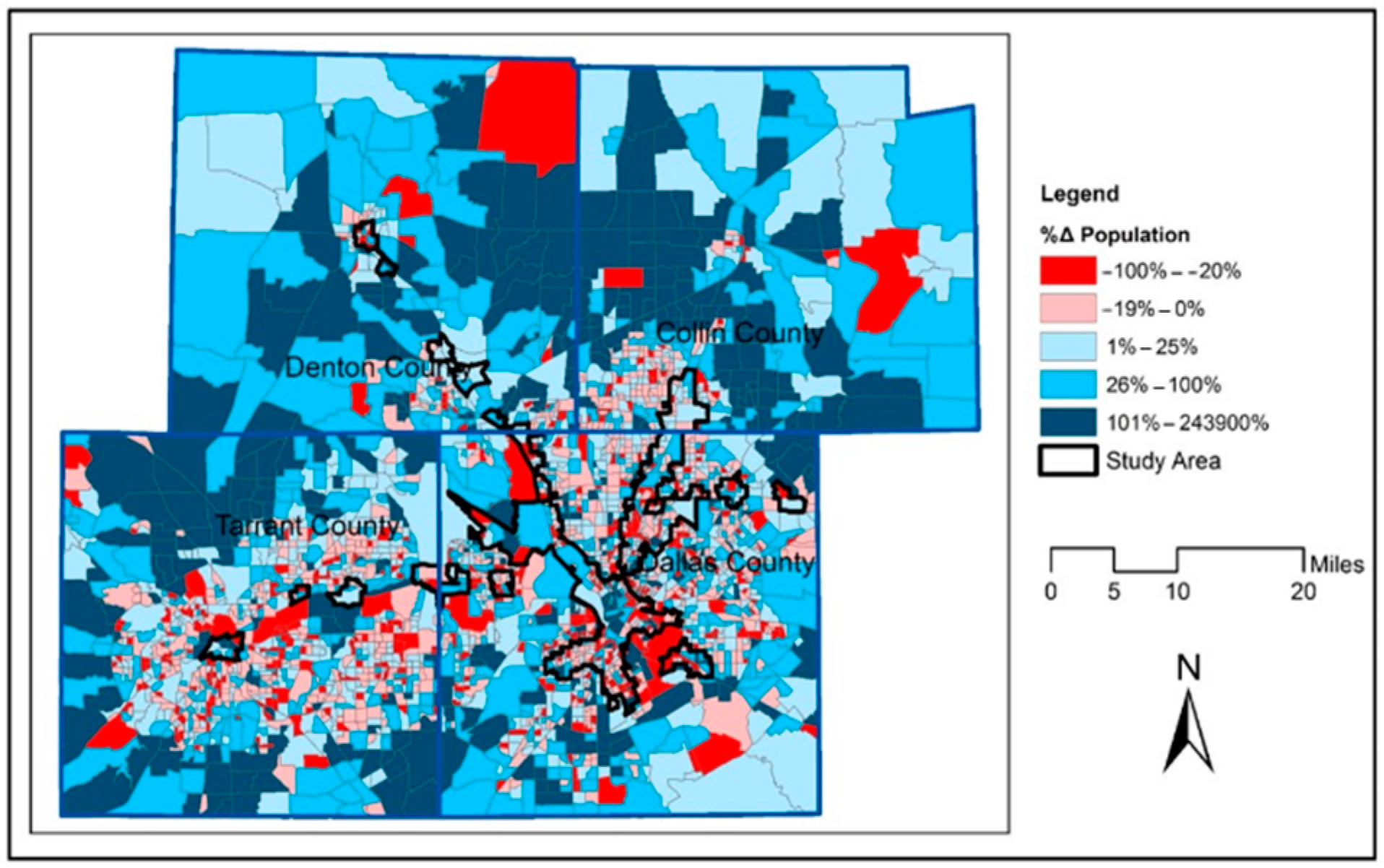
Table 2 shows that the block groups surrounding rail transit stations do not significantly increase their total population between 2000 and 2014, since many residents continued to move to the outlying areas. The median of the population density in 2000 was 1177 persons per block group, which increased to 1241 in 2014, a very small increase. Nearly half of the studied block groups experienced a negative percentage change between 2000 and 2014, most of which are located within the areas south and northeast of downtown Dallas and the surrounding areas near the Bachman, downtown Irving, and downtown Denton stations. However, a significant increase in the total population can be noticed in downtown Dallas, near the northern stations, and in some block groups within the city of Irving, as shown in
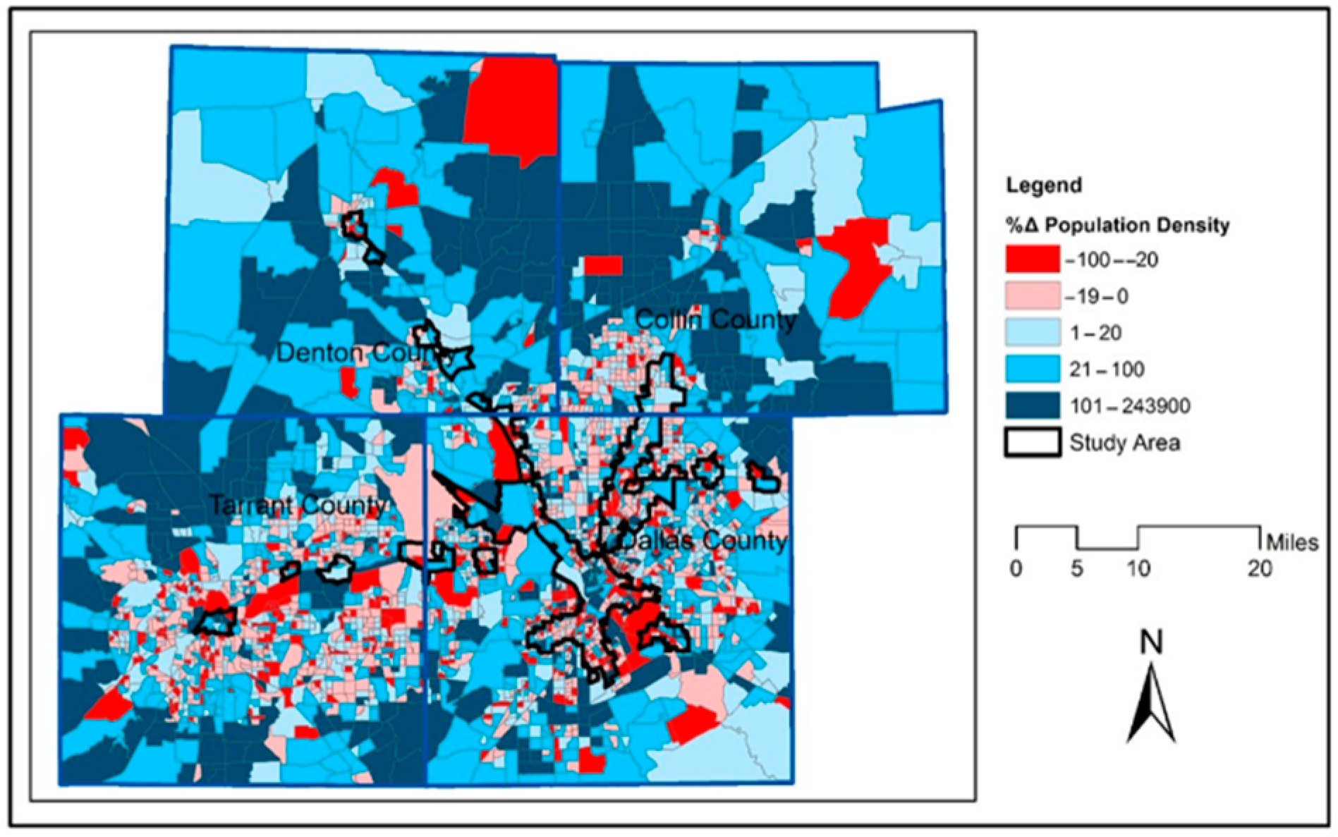
Figure 5. The median population density (the number of residents per acre) grew slightly from eight persons per acre in 2000 to nine persons per acre in 2014; in addition, 218 block groups show a negative percentage change in population density, while 236 show a positive percentage change. Generally, both the positive and negative percentage changes have a scattered distribution, with some concentration of adverse changes in the block groups located to the south and northeast of downtown Dallas, as shown in
Figure 6.
After adjusting the boundaries between 2000 and 2010 block groups, the four counties have 3064 block groups, as 2610 block groups are located in non-station areas. The Kruskal–Wallis test results show that all percentage changes in the selected variables are statistically significant at a 0.05 level of significance. This means that there are statistically significant differences between the percentage changes of the selected variables (the dependent and all of the independent variables) in block groups located within the study area and those found far from the station areas.
The comparison of station areas and non-station areas reveals the differences in changes that occurred between 2000 and 2014, as shown in
Table 3. It shows that the median of the total population and the median of the population density in the block groups within the study area are smaller than those in the non-station areas. In the non-station areas, the median increases significantly to almost 10% between 2000 and 2014.
Figure 7 and
Figure 8 show the increase in total population and population density between 2000 and 2014 within all block groups located in the four counties.
8. Regression Results and Discussion
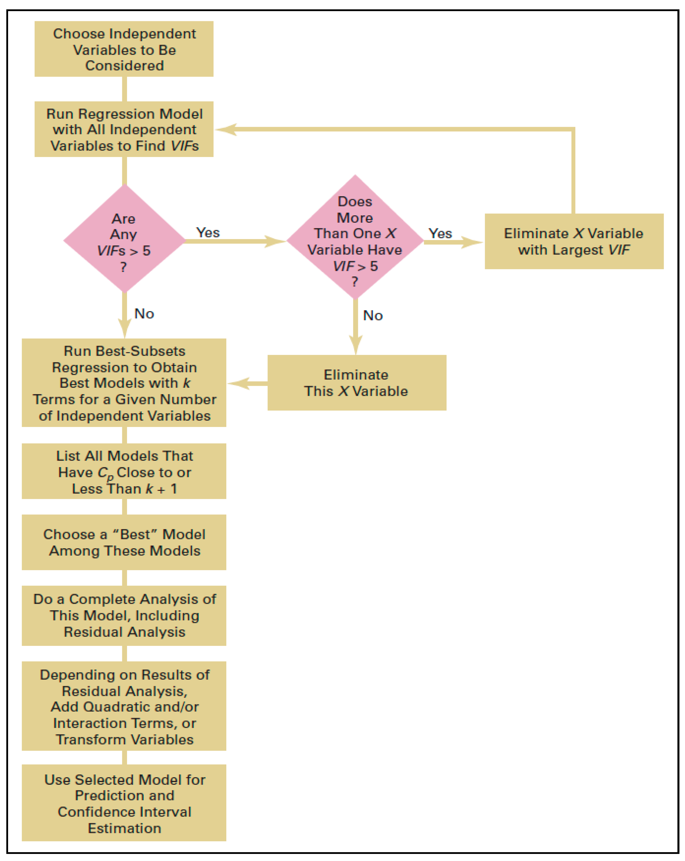
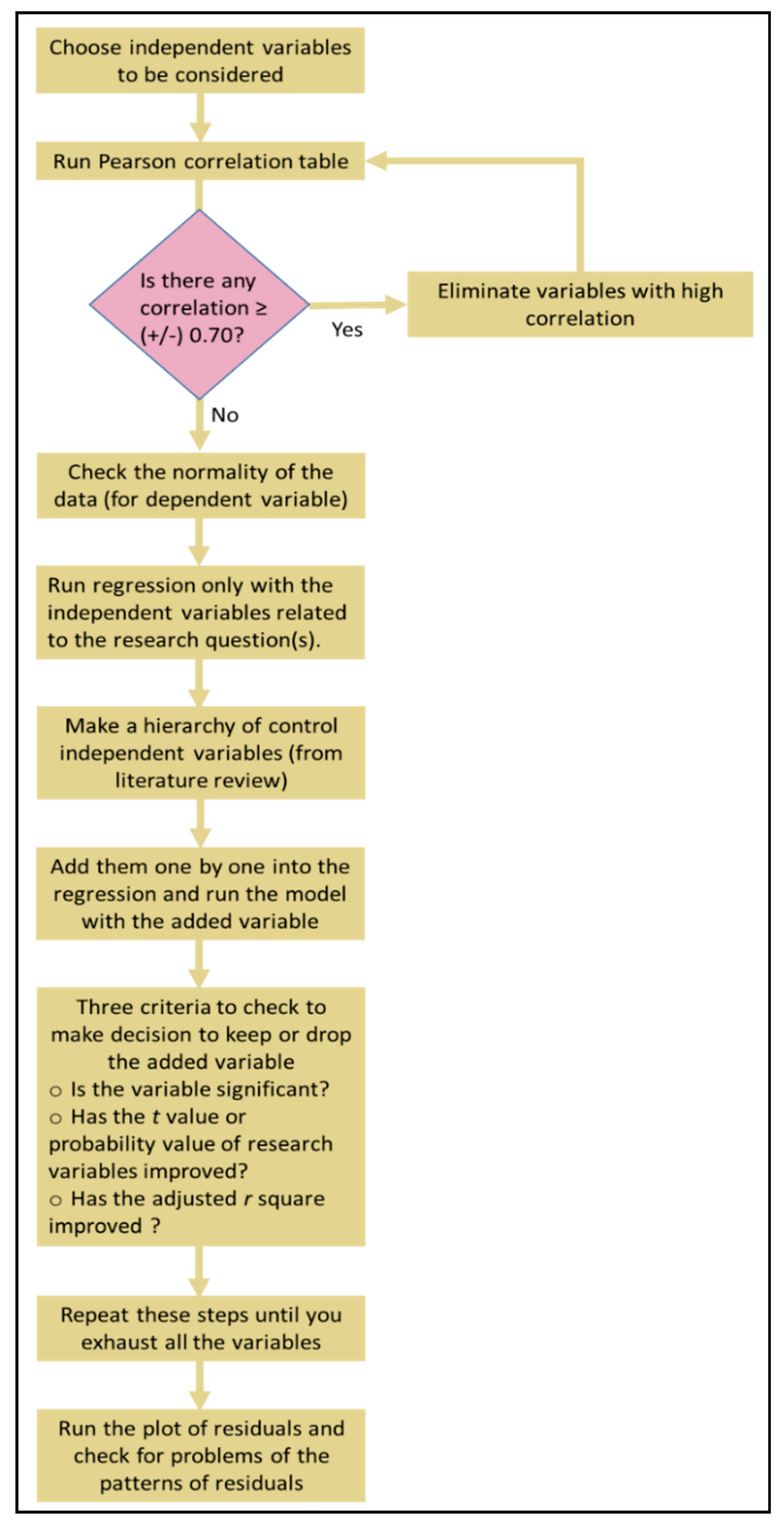
This section discusses some of the structured approaches to developing an appropriate regression model and then presents the best regression model results. Building a suitable model is a complicated process. Thus, Berenson’s model building [
59] (
Figure 9) and Anjomani’s modified version of model building [
60] (
Figure 10) are used to build the most appropriate regression model.
The first step is to identify whether or not the data are normally distributed; the test of normality is used for continuous dependent variables [
61,
62]. Thus, using Statistical Package for the Social Sciences (SPSS) to test the normality shows that the initial dependent variable (%ΔPopDen) is significant, meaning the data is not normally distributed. The residual analysis results do not show a normal distribution within the histogram, quantile-quantile (Q–Q) plot, or probability–probability (P–P) plot. Therefore, a transformation of data is used to achieve the normality of variables. We have tried many transformation methods, such as square root, square, and reciprocal, but we finally settled upon the most popular transformation method, the natural logarithm [
63]. However, there are positive changes in this study, negative and zero changes in some factors with which the logarithm is incompatible. Therefore, a conventional technique to handle zero value is to add a constant value, preferably 1, and then square the result to deal with a negative value; this is written as Ln(Δx+1)
2. No variables pertaining to distances have negative or zero values, and hence only the natural logarithm will be used. After this transformation, SPSS outputs show that the probability of dependent variables is more significant than 0.05; it means the data are normally distributed.
To measure the amount of collinearity between two or more independent variables, the variance inflation factor (VIF) is calculated, and the Pearson correlation table is analyzed to make sure that the multi-collinearity problem does not exist. Furthermore, the homoscedasticity test shows that the variance of errors is approximately constant, which means that the scatterplots are distributed randomly.
When we finished all tests, we used the regression model with only the independent variables related to the research questions and then add the rest of the independent variables, one by one, until exhausting all variables. The best model is determined based on the improvement of t-value, adjusted R2, the significance of the added independent variable, and the Cp statistic.
The natural logarithm is used to obtain the constant elasticity model. If the dependent and independent variables appear in the logarithmic form, this model is called the log–log; this means (1%Δx = β %Δy) [
62]. The other functional form involving logarithms in this study is the log–level model [
62], in which the dependent variable appears in the logarithmic form. In contrast, the independent variables stay in the original form. In this case, (Δx = (100*β) %Δy) [
62]. The major drawback of using the logarithmic form for the dependent variable is the difficulty in predicting the dependent variable’s original value. Therefore, the final model can be written as follows:
As shown in
Table 4, the regression model runs with the independent variables directly related to the research question, in line with model 1. Independent variables are added into the regression model—based on their importance and common usage in literature—one by one until all the variables are exhausted. As a result, the best model that explains population density changes next to rail transit stations after the analysis is model number 10. It has the highest adjusted R
2, and the Cp statistic in this equation is the closest to (K + 1).
The best model’s summary statistics with R
2 of 0.406 indicate that the independent variables explain nearly 40% of Ln’s variation (ΔPopDen + 1)
2 between 2000 and 2014. The highest adjusted R
2 is found in this model, which is 0.390, as shown in
Table 5.
The chosen multiple regression model results that include the coefficients and the corresponding significance levels are shown in
Table 6. Most of the coefficients are statistically significant at the 5% level. Consequently, the null hypothesis can be rejected at a 95% confidence level, and these variables are representative of the population. Transportation accessibility variables show different coefficient signs; see
Table 6. Unexpectedly, the relationship between the distance to a rail station and population density is positive. This means that a 1% increase in the distance from a rail transit station to the centroid point of a block group is likely to increase Ln(ΔPopDen + 1)
2 by 0.472. This translates into an approximate 0.27% increase in population density between 2000 and 2014 for a 1% increase in the distance from a rail transit station, having all independent variables as fixed. To keep the interpretations simple and avoid confusion, the “change” from the name of the variables will not be used. As expected, the coefficients of distance to a highway ramp and the distance to the closest city center are negative. An increase of 1% away from the nearest highway ramp to the selected block group leads to a 0.105% decline in population density, taking all independent variables constant. Moreover, a 1% increase in the distance between the closest city center and the selected block groups decreases the population density by 0.05%, holding all other independent variables as fixed. This means that the shorter the distance to a highway ramp or city center, the higher the population density.
In the model, all variables related to the residents’ socioeconomic attributes positively correlate with the dependent variable. The number of employed residents, white residents, and Hispanic residents are the most significant independent variables among the socioeconomic variables. A 1% increase in employed residents within the study area increases the population density by 0.216%, holding all the other variables constant. Moreover, a 1% increase in the number of white dwellers within the selected block groups next to rail stations leads to, on average, a 0.189% increase in population density per acre between 2000 and 2014. Furthermore, a 1% increase in Hispanic residents has an increase in population density of approximately 0.248%, while the impacts of all the other variables are held constant. These imply, as expected, that a thriving station area would attract employed people of a different race or ethnic group. Interestingly, these three variables’ bata value is the highest among all the independent variables, indicating that the socioeconomic attributes are the most important contributors to the population density increase in the station area. As is discussed below, the following high beta value belongs to the TOD, if the station is a transit-oriented development, which completes the socioeconomic picture depicted above—a thriving station area attracts mixed-use developments of a TOD and people with jobs of mixed socioeconomic groups.
Change in poverty level has a negligible impact on population density in the block groups in question. With a 1% increase in poverty levels, population density increases by 0.089% while controlling for all other variables. Only the median housing value variable becomes significant among the variables related to housing market variables. In this model, a 1% increase in the median housing value results in a 0.080% increase in population density per acre. This demonstrates a very small impact on population density.
Independent variables related to location attributes show the expected signs. The number of jobs variable shows a negative sign; this means that as the number of jobs within the selected block group increases by 1%, the population density declines by 0.060%. Only one dummy variable within this model becomes significant—whether the rail station has been developed as TOD or non-TOD—and the coefficient sign is positive, as expected. The coefficients have a percentage interpretation; population density in block groups developed as a TOD is 100 × [exp(0.454) − 1] = 58% higher than the population density of block groups that are considered non-TOD in the period between 2000 and 2014.
9. Findings and Conclusions
The results indicate that the population density does not significantly change the block groups within the study area compared to block groups away from the station area. Considering the region’s rapid growth, suburban areas’ attractiveness in this car-oriented large metropolitan area is highlighted.
However, the regression analysis produced some interesting findings, as will be highlighted in this section. A positive correlation is shown between population density and living farther from the rail transit station when independent variables are used. A minor change is noticed in population density living closer to the station. A possible explanation is that block groups close or next to rail stations have fewer residential uses and thus a lower number of people per block group. This supports what many authors suggested—that urban transit systems rarely increase accessibility in auto-dependent cities. Moreover, one possible explanation is that only passenger transit systems are provided for small areas within the DFW area than the low density and large size of the whole metropolitan area. However, even if passenger transit services were widespread, an increase in population density is unlikely to happen next to rail stations because the DFW area is an automobile-dominated metropolitan area with an extensive highway network.
The distance between the city center and the nearest highway access ramp negatively relates to population density change. This means that areas close to the highway ramps or city centers have a higher population density change than those located farther away from the highway ramps or the city centers. As discussed in the literature, the improved accessibility generated by highway ramps and city centers can play a major role in increasing population density [
36].
The results also show that as the change in the number of employed residents, white residents, or Hispanic residents increases, the change in population density increases. Some of the study area residents are middle-class, white, or Hispanic workers who live in smaller homes or apartments. They benefit from easy accessibility provided by rail systems, which can help reduce commuting costs and time and avoid traffic congestion. As was also hinted in the statistical results, these three independent variables, followed by the TOD variable, had the highest score for beta values, which indicated they are the most important or critical factors affecting the increase of density in the station areas.
Changes in median housing value are positively correlated with changes in population density. These results confirm what theories and literature have found. In theory, higher land prices will be compensated with higher density, and more housing units will be developed in each parcel. Changes in the number of jobs are negatively correlated with changes in population density in areas surrounding stations. In effect, substantial commercial, administrative, and industrial uses can utilize more land, resulting in a lower percentage of residential uses and thereby lowering population density.
Again, the beta values variables with high positive beta coefficients are the percentage change in Hispanic residents, change in employed residents, change in white residents, and TOD. These variables display an interesting collection of policy-related factors regarding implications for increasing density in the station areas. Developments and policies that increase racial mix and employment opportunities with mixed-use TOD commercial activities will increase residential density in close vicinity to the station. This would attract employed people of a different race or ethnic of diverse socioeconomic groups while enhancing commercial activities to further economic growth and transit use in the region.
In short, changes in population density are influenced by proximity to rail stations. However, many other factors such as proximity to highway access ramps and city centers, residents’ education, employment, race, ethnicity, and related attributes impact population density.
As was mentioned in the modeling section, there were challenges in model building and data preparation since the study looked at a relatively long 15-year period, a change between 2000 and 2014. To overcome these and build the most appropriate model aside from statistical scrutiny, we used Berenson’s model building procedure [
61]. However, while we were aware of fundamental challenges in empirical research such as controlling for unobserved heterogeneity, fixed effects, and common errors [
62,
64,
65], we did not control for consistency or fixed effects estimator because of the complexity of the Berenson’s process [
59,
60], which is a limitation of our analysis.
10. Recommendations
Only very few residents (0.6%) who live next to rail transit stations commute by rail transit since the DFW area is characterized by auto-oriented and low-density developments. In addition, the rail transit system in the DFW area only covers the major cities, it is very slow with few frequencies, and passengers have to wait for a long time on the stations and transfer areas. Thus, urban planners and policymakers should suggest some solutions to increase population density, attract more diverse populations to the study area, increase transit ridership, and sustain station area development.
Policymakers should adopt a TOD development policy to capitalize on creating compact, mixed-use, mixed-race and ethnicity, high density, and making housing in neighborhoods adjacent to rail stations affordable. City planners can also practice TODs through specific procedures such as rezoning industrial and warehouse uses, utilizing unused land, and redeveloping projects located close to rail stations in zones that permit higher density. Moreover, policymakers should support future transit stations by adopting transit-supportive land-use policies that support higher density clusters rather than supporting low-density communities that stimulate sprawl patterns, which, in turn, increase the dependency on automobiles.
Developing communities near rail stations as TODs can be achieved by promoting a contemporary urban design and utilizing facilities such as the station location, parking lots, streets, edges, pedestrian trails, and station plazas. The ideal urban design of TODs can increase transit and encourage transit ridership, reducing automobile dependency.
Moreover, the improvement of rail transit coverage and transit quality is a significant factor in increasing transit ridership. Residents sometimes avoid commuting by rail transit since they perceive it as an unsafe, inconvenient, uncomfortable, and unreliable means of transportation [
63]. Accordingly, transit agencies and decision makers should consider improving the quality of rail transit system services within the DFW area. This also means that these systems should cover a large extent, provide better services, and have shorter waiting times, more frequent services, and greater speed.
The DFW metropolitan area can be considered an auto-oriented environment where public funds are primarily directed toward highway improvement. Moreover, an improvement in transit access and quality needs to be incorporated into regional and local policies alongside the other implementation measures to prioritize this improvement.


