Abstract
Nowadays, even with the growth and progress of the agricultural sector, the food gap (FG) is still wide, particularly for strategic crops, affecting the national economy and compromising the food security. The realization of self-sufficiency can be fulfilled only by achieving the highest production efficiency along with preserving the natural resources currently available, especially arable land and irrigation water. In this analysis, the FG in Egypt was modeled for 13 crops between the years 2000 and 2018. The linear model applied suggested a redistribution of crops in terms of production, food demand and land reallocation, in order to find the best solution to minimize the FG on the basis of crop value and under a set of constraints. It was found that the value of the modelled FG increased steadily from 2005 to 2017, then it started to decline slightly, probably due to the steady increase in the population growth rate which is a crucial factor in enlarging the FG. Furthermore, important water loss was noticed through the analysis period. In fact, there was a huge difference, reaching around 25 billion m3 between the water consumed for the studied crops and the total amount of renewable water. The main reason for this loss can be linked to the traditional irrigation methods used, such as surface irrigation. Moreover, the calculation of food demand with the estimated production and the redistribution of crop land reallocations were performed to achieve the best model fit between the crops in terms of minimizing the FG in Egypt. So far, the current agricultural policy has reaped limited gains and a steep decline of food economic balance. Hence, significant interest on rising productivity should be given by the government to achieve the food self-sufficiency in Egypt.
1. Introduction
Food is considered the primary necessitate for human needs. This need is based around the work of economic sectors such as agriculture, industry and trade, thus, food security is a significant issue that represents the usefulness and efficiency of sustainable development policies (economically, socially and environmentally), especially in light of the demand increase in food products and the continuous rise in their prices, which is accompanied by the increase in the number of people and their change in consumption patterns [1,2].
Food security is of paramount importance in times of economic, natural and human crisis due to shifts in food supply and demand, scarcity of food, lack of consumer stability and loss of income, all of which are among the factors affecting the essence and content of food security [3,4].
On the other hand, food security is a complex and interrelated issue [5]. It is a holistic issue whose dimensions overlap in most economic, social and environmental sectors, and it is defined as one of the main goals of any development process, as it is reflected in important development goals, related to living the human, health and expected age [6,7]. Consequently, the dimensions of food security are related to the dimensions of economic development (agriculture, industry, trade, prices, etc.), social (poverty and human development, especially the health dimension, etc.), the environmental dimension related to climate and desertification and its impact on agricultural production, and the food security related to population stability and commodity stability [6,7,8].
According to the World Food Security Summit in 2009, food security is achieved when all people, at all times, have physical, social and economic opportunities [9].
As for food insecurity, it is the situation in which people lack access to adequate quantities of safe and nutritious foods, to ensure a normal and healthy life [9].
Herein, it is necessary to distinguish between two levels of food security (absolute and relative):
- Absolute food security means the production of food within a single country equivalent to or greater than local demand, this level is synonymous with complete self-sufficiency, or complete food security. It is clear that this absolute definition is not realistic, as the state is missing out on the ability to benefit from international trade based on specialization, division of labor and the exploitation of comparative advantages [10,11].
- Concerning relative food security, this means the ability of a country, or a group of countries, to provide commodities and foodstuffs partially or totally. This is in the sense of providing the society’s needs of basic food commodities, partially or completely at a minimum, as it does not mean the production of all the basic food needs; rather, it is to provide the necessary materials to secure these food needs, in cooperation with other countries [12,13].
Indeed, the components of food security are present in a country that owns favourable geographic and climatic characteristics, an abundance of water resources, human resources, agricultural lands, pastures, forests, livestock, and a modern technology [14,15].
The reality of the Arab countries requires that they provide food security to their citizens, at least. If we take Egypt, it was once considered the food basket of the Arab world and is a historical model of food self-sufficiency, due to the availability of large agricultural areas and the abundance of labor [16]. Egypt relied on beans and wheat during the historical crises, but today, it has become one of the largest importers of these two commodities [17,18].
The definition of a food gap (FG) is the disproportion between the required food quantities and the population, which leads the concerned country to import food from abroad, thus any shortage of food resources is matched by an increase in the population [19].
Many research papers have been published on the study of the FG and ways to reduce it in Egypt; most of these studies discuss the main crops such as wheat and maize, which are highly consumed in Egypt and their production does not cover the local market [20]. Other studies explain the factors that contribute to widening the FG, for example, the limited investment in agricultural and food projects [21], and the impact of climate change and water scarcity on the FG [22,23].
In the fifties and sixties of the last century, a large number of simulation and optimization models have been used for the appropriate planning and management of water use in irrigated agriculture and FG [24,25]. Soon after the simplex algorithm was found by Dantzig in 1947 [26], agricultural economists started to use linear programming for farm planning. Early publications related linear programming in agriculture as one of the best tools for the optimal allocation of land and water resources [27,28] either aimed at disseminating the mathematical knowledge by explaining the characteristics of the procedure [29,30] or at pointing out its possible applications and general potential for farm management [31,32] and applied linear programming to the hypothetical agricultural holding in order to find optimal production plans by minimizing the FG in a country [33].
In this research, we will calculate and analyze the FG during 2000–2018, as well as the water consumption for the crops studied and food demands for the country. Additionally, we will reallocate the land cultivations under a set of constraints to reduce the FG.
The problem of the study is as follows:
- Egypt as a developing country is facing a crucial challenge in providing the citizens’ needs of basic food commodities to keep pace with the steady population growth. To that end, it should work to raise the productivity of the agricultural sector in order to achieve self-sufficiency and to lessen food imports. The FG that affects the staple commodities is a major problem for the state that bears the burden of providing a high budget to stipend the importations usually being paid for with foreign currency. This requires studying FG for the most important crops that represent the biggest portion in the contribution of the national food security in Egypt.
The objectives of the study are to:
- Determine and calculate the FG during 2000–2018 for the most important food crops in Egypt;
- Determine the water consumption and the food demand for the same study period;
- Build a mathematical model to find the optimum land reallocation and production distribution for minimizing the FG.
2. Materials and Methods
The data used for this study describe several variables in relation to thirteen crops for the period between 2000 and 2018. The data were collected and used in all calculations (area, crop yield, crop exports, and crop imports,) from the on-line database of the Food and Agriculture Organization of the United Nations (FAOSTAT), World Bank Open Data, Central Agency for Public Mobilization and Statistics (CAPMAS) of Egypt. In addition, the average world market prices USD/ton was collected from the World Bank Open Data and “Water footprints of nations Volume 2: Appendices” [34].
Regarding the statistical analysis, it was performed by using Stata software. In this part, the linear relationship between the water consumption and the FG will be assessed and modelled for a period of nineteen years (2000–2018).
2.1. Crop Water Requirements
The crop water use for each crop included in the study were calculated with the following equation (Equation (1)):
where:
CWR: the amount of water requirements for each crop (c) measured in the field in m3/hectare (ha) Table 1. It is defined as the amount of water required for evapotranspiration from the planting until the harvest for a specific crop that grows in soil containing sufficient water for it., The crop evapotranspiration (ETc) under standard conditions was calculated following the crop evapotranspiration guidelines for computing crop water requirements [35]. No limitations are placed on crop growth or evapotranspiration from soil water and salinity stress, crop density, pests, and diseases, weed infestation or low fertility. ETc is determined by the crop coefficient approach whereby the effect of the various weather conditions are incorporated into ET0 and the crop characteristics into the Kc coefficient”. The water requirement is assumed to be constant for each crop.

Table 1.
Crop water requirements (CWR) for the studied crops.
Production: production of crop (c) measured in tons.
Yield: yield of crop (c) per unit area, measured in tons/ha.
The quantity of water requirements of crop (c) is calculated from the following relationship Equation (2):
where:
The factor 10 is meant to convert mm into m3/ha, and the summation is carried out over the period from the first to the final day of the growing period.
lp: represents the length of growth, measured in days.
Etc: is the amount of daily evapotranspiration of the crop (c) and it is measured in mm. This evapotranspiration is obtained by the process of multiplying the reference evapotranspiration amount ET0 by the coefficient of the crop Kc. The crop coefficient is taken from four stages of the crop growth; initial, crop development, mid-season and late season, that is the stage where the crop is ready for harvest [35,36].
ETc (c) is the crop evapotranspiration [mm d−1].
Kc (c) crop coefficient indicates the relationship between the evapotranspiration of the crop (ETc) and the reference evapotranspiration (ET0).
ET0, the amount of reference evapotranspiration, which is the percentage of evapotranspiration from the grass in specific growth conditions, is affected by climatic conditions only [37] [mm d−1].
The water consumption of crops varies according to their growth stage. In fact, the water consumption is at a low rate at the beginning of the crop growing season, when it is mostly in form of evaporation from the soil surface, then it increases with the plant growth as a result of the leaf mass surface increase and is consumed in the form of transpiration from the leaves up to the maximum growth stages. Kc differs according to the type of the crop, the growth phase, the growing season, and the associated climatic conditions. Kc expresses the effect of the properties that distinguish the field crop from the reference grass, whose appearance is stable and covers the entire ground, and therefore different crops have different Kc.
Several weather condition effects have been incorporated into the ET0, that then represent an indicator of the atmospheric requirements needed for the process of evapotranspiration from green grass surfaces. Accordingly, the Kc varies greatly with the characteristics of the crop and to a small extent with the climate. Thing that can explain the possible transfer of the Kc values that were calculated at one of the irrigation research stations for generalization between sites and climatic regions by Hargreaves and Merkley (1998) [38] to the ET0 reference. The ET0 represents the evaporating potential of the atmosphere at a specific spatio-temporal point and disregards the crop features and soil factors [35].The ET0 was calculated as an average of all the months of the year through the CROPWAT program [39,40]. As for the Kc values, they were derived from a previous study performed by the researchers Allen et al. (1998) [35] and Champagain and Hoekstra (2004) [41].
2.2. Describing the Mathematical Model and the Resources Constraints
Mathematical modelling is an approach allowing one to assess and to understand any system interactions, as well to solve optimization problems along with different constraints. In such problems, the decision maker aims to optimize the solution according to some criteria and limitations.
In other words, a mathematical model can be used for optimizing f(x) under the constraint g(x). Particularly, if f(x) and g(x) are linear functions, the problem will be linear. Correspondingly, the agricultural activity problems are usually evaluated through linear programming [42]. In the present study, the optimization of the system studied seeks to minimize the FG (Equations (4) and (5)) under four different constraints.
Considering that we are assessing several key crops of economic importance, we aim to reduce the FG that is expressed by the disproportion between the required food amounts of the population and the local production, which leads the concerned country to import food from abroad [19]. The FG optimization means the production optimization according to the limited resources and the population need increase. In the model created in the scope of this study, we tried to reorganize the factors that contribute to the widening of the FG, such as the crop area that can be re-allocated on the basis of different aspects in relation to the crop value and the population needs.
The objective of our model is to determine the so-called “objective function”, that is a function of unknown crop area reallocation (ha) Aj, which is expressed mathematically as the following:
Dj: The amount of food demand for each crop j (ton). It can be calculated following the relationship Equation (6):
Ij, Ej, Sj are, respectively, imports, exports and productions of each crop j (ton).
Prij: International crop price (USD per ton) from the World Bank Open Data and [41].
Proj: Productivity of each crop j (ton per hectare).
NC: Number of crops.
The minimization of FG is modelled, taking into consideration a set of constraints, that are as follows:
- The area allocation set for each crop should be positive, this constraint is known as the non-negative variable (Equation (7)):
- The total crops land allocation should not exceed the maximum exploitable land (Landconst = 3.5 million hectares) (Equation (8)):
- The total crops water consumption should be less than the renewable water volume (Waterconst = 45 billion m3) (Equation (9)):CWRj: Crop water requirement for each crop j (m3 per hectare).
- The production of the allocated area should not exceed the required amount for each crop (the demand) (Equation (10)). Actually, this constraint is necessary, especially for the strategic crops in order to determine the volume of production for each crop which have a high economic return whose production may exceed the market need in Egypt [43]:
As mentioned previously, the problem consists of finding the crops’ area reallocation Aj that minimizes the FG per year. We say that a constraint is saturated when the optimal solution uses the total available resources.
The first algorithm used for solving linear programs was presented by Dantzig in 1947. We used the so-called simplex algorithm even though there are many competitive alternative algorithms at the present time. By the means of the programming language named “Octave” and the package “GLPK” (GNU Linear Programming Kit), our linear programming (LP) problem was successfully solved, and the model output expresses the optimum land reallocation for minimizing the FG.
The model was applied on two types of data (average and annual) only for the production and food demand. A temporal evaluation of the model outputs was established to follow the fluctuation of the FG, the water consumption, and the crop land reallocation throughout the study period.
3. Results and Discussion
As it was disclosed previously, our model outputs express the optimal propositions in terms of crop area reallocation, in such a manner to reduce the FG as much as possible depending on several constraints. Mentioning that, the constraint for the total cultivated land was saturated in all the proposed scenarios.
3.1. Crops Land Reallocation for the Studied Crops during 2000–2018
As mentioned previously, the problem consists of setting a new crops’ area al-location (Aj) that minimize the FG per year. The area for the whole crops should not exceed the total available area in the country which is equal to 3.5 million hectares. Figure 1 represents the real allocation of all crops through the studied period while Figure 2 illustrates the model output, indeed, all the crops except rice, wheat, potatoes, sugar beet, and maize, are reallocated fairly close to the real situation. Mostly, the crops that are similarly distributed converge to the maximum allowed area (for non-exceeding the crop demand). The excepted crops are critical, in which their allocation is affected by the policy followed by the government as well as other factors, some of which were mentioned heretofore.
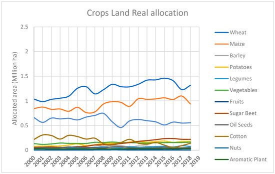
Figure 1.
Crops land real allocations for the studied crops.
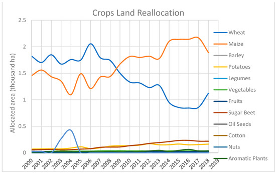
Figure 2.
Crops land reallocations for the studied crops. Resource: own calculating.
As it is known, land allocation refers to assigning land to be used in a certain manner, however, it may not mean that the actual use of the land reflects the initial plan of its allocation [44]. That is what happened with rice, wheat, potatoes, sugar beet and maize crops in Figure 1.
3.2. Food Gap
From Figure 3, it is clear that the FG has increased with the years, starting from 2005 to 2017. This that can be explained by several reasons in relation to different aspects. In fact, the steady increase in the population growth rate is an important factor amongst others in the widening of the FG, particularly for the period from 2000–2018, during which it had reached 2.56% according to the Central Agency for Public Mobilization and Statistics in Egypt, ensuing an increase in the food demand notably for strategic crops such as wheat, maize and rice. Furthermore, the global financial crisis in 2008 engendered volatile global prices for these strategic crops. Additionally, the technical integration of the production procedures is still low and does not cover the whole cultivated area [45]. Over and above, there are two important aspects of the widening FG in Egypt for these crops:
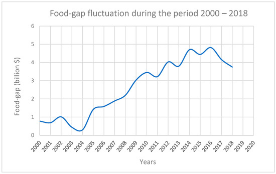
Figure 3.
Food gap fluctuation of some important crops for the period between “2000–2018”. Resource: own calculating.
Firstly, the supply in the food market (the adopted agricultural policies, the loss of agricultural production and its impact on public consumption, the availability of agricultural production requirements, the agricultural sector’s share of investments, environmental problems and climate change, the costs and prices of crop production, and government support provided to farmers) [46,47].
Secondly, demand in the food market (population increase and growth as mentioned above, per capita national income, price policies adopted, customs, traditions and consumption patterns, migration and economic openness of the country) [48,49]. All these reasons have led to the widening of the FG in Egypt recently.
3.3. The Water Consumption for the Studied Crops
The mathematical model applied under different constraints gave us an estimation of the water consumption of the studied crops considering their CWR. One of the model constraints is that the water consumption of the crops should not exceed the renewable water resource for the agricultural sector in the country and that is about 45 billion m3. Through the analysis period, a huge difference, reaching around 25 billion m3, between the water consumed for the studied crops and the total amount of renewable water (Waterconst) was observed (Figure 4). Even though this water amount difference is supposed to be exploited to irrigate other crops, it is clear that there is an important water loss. This can be explained by several reasons, including the traditional irrigation methods as well as the used technique such as surface irrigation in many nearby areas of the Nile river, where the water use efficiency is very low [50]. In addition, the lack of use of modern technology skills in irrigation and the lack of guidance for the farmers through the establishment of introductory courses that contribute to teaching them some methods about using modern irrigation that reduce the water waste, such as sprinkler and drip irrigation [51]. This is as well as the environmental impact (high temperature, low precipitation), especially for the crops which need high amounts of water.
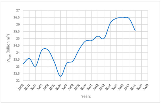
Figure 4.
The water consumption for the studied crops. Resource: own calculating.
3.4. Statistical Analysis for the Food Gap and the Water Consumption
Figure 5 reveals in a better way the trend between the FG and the water consumptions during 19 years for the studied crops. We noticed that the variation is a direct proportion between water consumption and the FG, and this can also be proved statistically by modelling them through SPSS program using the simple linear regression (LR) model.
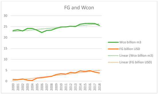
Figure 5.
The FG and the water consumption trend for 19 years’ period. Resource: own calculating.
- The response variable (dependent variable) is the FG;
- The covariate (independent variable) is the water consumption (Wcon);
- The observations (OBS) from 2000 to 2018.
The question was to check whether the water consumption was a significant variable to explain the FG changes, or not.
Simple linear regression was used in order to determine the influence of the independent variable Wcon on a dependent variable FG. In addition, it was necessary to transform the data by Square Root Transformation (SQRT), since there is a noticeable moderate negative skewness in the studied data [52]. The results are reported in the Table 2 and they can be expressed in the following regression Equation (11):
FG = 8986.700 + 26,877.114 Wcon + e
Table 2.
The LR model applied on the studied data.
The intercept value shows the influence of Wcon on FG. It means that if all the independent variables are zero, FG as the dependent variable is predicted to be 8986.700. Furthermore, the value 26,877.114 represents the coefficient of Wcon, obviously meaning that if Wcon increases by one unit then FG is predicted to increase by 26,877.114.
Afterwards, the test of goodness to fit was used Table 3. Based on the analysis, the correlation coefficient (R) is equal to 0.875 indicating the strong relationship of independent variable to the dependent variable. The coefficient of determination (R2) is equal to 0.766, which means that the independent variable affected the dependent variable with 76.6% in this model.
Table 3.
Test of goodness of the LR model applied on the studied data.
A classical assumption test was needed to ensure that there was no impediment to use the regression analysis, verifying the homoscedasticity, the normality and the autocorrelation.
Figure 6 shows that the pattern of points is spread from both sides of the zero line of the ordinate, revealing that there is no heteroscedasticity in this regression.
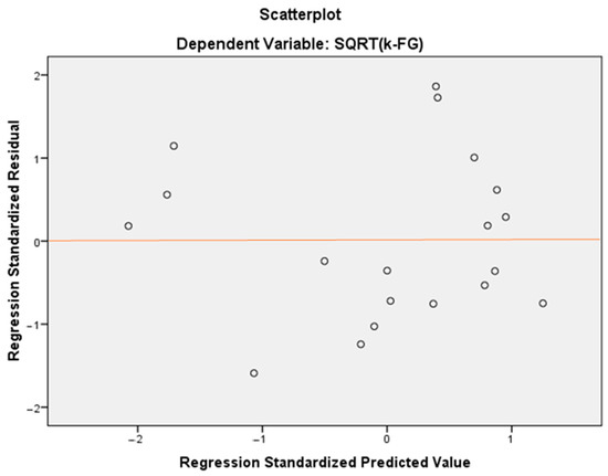
Figure 6.
The heteroskedasticity of the residuals resulted from the LR model applied on the studied data.
Later, the normality test was used, and the resulted graph Probability Plot plot (Figure 7) shows that the expected values are strongly correlated to the observed values of the FG.
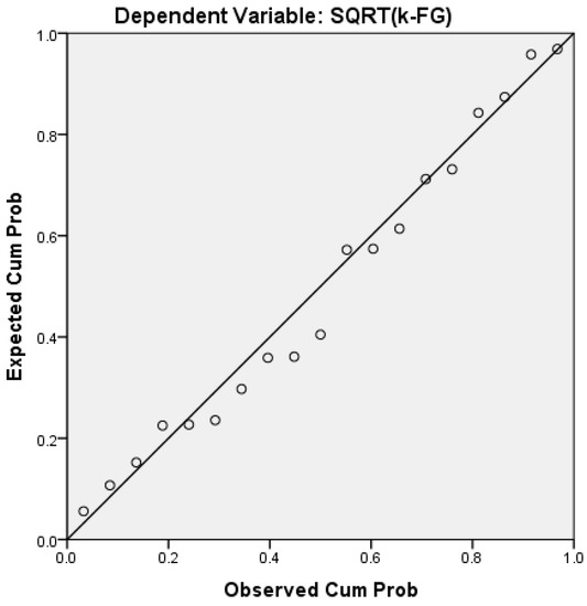
Figure 7.
Normal probability plot of regression standardized residual displaying expected vs. observed values of the studied data using LR model.
Additionally, we used the Shapiro–Wilk test since the data observations are less than 50 [53]. In this test, we set the following assumptions:
- If the value of Shapiro–Wilk (sig.) > 0.05, this means that the data are normally distributed;
- If the value of Shapiro–Wilk (sig.) < 0.05, this means that the data are not normally distributed.
Table 4 illustrates the (sig.) values of the Shapiro–Wilk test for both variables, are > 0.05. This means that the data can be said to be normally distributed even though the data are at risk of a lower bound of true significance because of its small size.
Table 4.
Tests of normality resulted from the LR model on the studied data.
Later on, the autocorrelation test (the Durbin–Watson (DW)) was used to determine the correlation of variables in the regression model along the time.
Based on the Table 5, we can see that the DW value is equal to 1.915, which means there are no autocorrelation symptoms in the current model.
Table 5.
Durbin–Watson test for autocorrelation of the residuals resulted from the LR model on the studied data.
Finally, the hypothesis test is intended to determine the effect of Wcon as the independent variable to the FG as the dependent variable. The Ttest is used to determine the partial effect of the independent variable on the dependent variable. This test is carried out by comparing the Tcount with the Ttable with the level of significance of 95% (α = 0.05). The assumptions of this test are as follows:
- If the Tcount > Ttable or sig. (p-value) < 0.05, then the variable Wcon influences FG;
- and if the Tcount < Ttable or sig. (p-value) > 0.05, then the variable Wcon does not influence FG.
Table 6 displays that the Tcount is 7.468. The Ttable is 1.729 (n = 19, p = 0.05); the result is Tcount > Ttable, and the sig. (p-value) is also < 0.05. It means that the variable Wcon is significantly influencing the FG variation.
Table 6.
Ttest applied on the studied data.
3.5. Average Demand and Production of the Crops during the Period 2000–2018
The calculation of the crop demand allowed us to re-estimate the productions with the aim to achieve the best model fit between crops in terms of minimizing the FG in Egypt. This analysis was performed by taking into consideration the annual average of the variables used during the 19-year period (2000–2018). Our model recommended the best solution in comparison to the real situation of the crops production. Figure 8 illustrates an analogy between the calculated average demand and the recommended average production of the studied crops during the 19-years period. For many crops such as maize, potatoes, sugar beet, legumes, vegetables, fruit, nuts, and aromatic plants, we notice that the production is equal to the demand, which reflects the saturation of the constraint (the maximum production should not exceed the demand for each crop for the reason mentioned above). For the wheat, barley, rice and cotton crops, their demands are higher than their productions. This can be elucidated by the fact that the above-mentioned crops (especially cotton and wheat) are more valuable in Egypt, thus their price is higher as well. Consequently, the government revenues benefit from purchasing these valuable crops from the farmers at reasonable prices and then exporting them at high prices besides importing other varieties with lower prices and in larger quantities, in order to achieve the economic balance in the country [54].
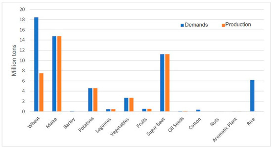
Figure 8.
The average demand and the average recommended production of the crops. Resource: own calculating.
3.6. The Deficit between the Crop Demands and Production of the Crops from 2000–2018
With regard to the mathematical model used, the main goal is to reduce the FG in the country as much as possible for thirteen important crops. After calculating the annual productions and demands redistribution for minimizing the FG, the new resulted annual production amounts were subtracted from the new annual demands, to assess the deficit produced from the suggested redistribution carried out by our linear model on the basis of the crops’ priority. As the production for each crop should not exceed the demand, we have determined the term deficit as the difference between the demand and the production. In the best case, the deficit is equal to zero, which means a self-sufficiency was reached for that crop. With regard to the four crops mentioned above, the results were not equal to zero. This result can be related to several factors, among which are the preferences of the farmers in terms of choosing these crops over the years, and the political strategy issues related to the economic balance and the laws applied on exportations and importations of the country (mentioned above). To achieve the self-sufficiency in the agricultural sector at the long term, considering only some strategic crops in this study, we can say that the suggestions provided by our mathematical model can be considered as ideal solutions if applied appropriately, regardless the political conditions of the country. Indeed, Figure 9 illustrates the deficit between the crops demand and the production from the year 2000 to 2018. For all the crops, the deficit in the suggested model resulted in zero, except for the wheat, barley, cotton, and rice crops.
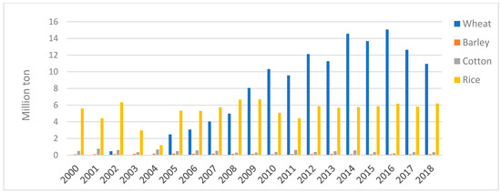
Figure 9.
The deficit between the crops’ demand and production of the crops from 2000–2018 for the wheat, barley, cotton, and rice crops. Resource: Own calculating
4. Conclusions and Recommendations
In this study, we have concluded important results that may help the government and/or the decision-makers to improve the reality of agricultural production and farmers.
By calculating the FG from 2000–2018, we noticed an increased with the years, starting from 2005 to 2017. Maybe the essential reason was the increase in the population growth rate that has led to an increase in food demands.
Through the estimation of water consumption and the comparison with renewable water resources for the agricultural sector in the country, an immense difference, reaching around 25 billion m3, between the water consumed for the studied crops and the total amount of renewable water was detected. Perhaps the reasons for this may be in the traditional irrigation methods used to irrigate crops, where water losses are large and also have environmental causes.
We also noticed that the FG and water consumption are positively correlated over the years and that was proved statistically. The model was quite good in predicting the FG variation, nevertheless, it needs to be improved by incorporating other significant covariates adding fair contribution to recompense the error term. Likewise, the available data were restricted to a 19-year duration, which gives a quite small number of observations needed for a better statistical analysis.
The main objective of the study was to identify the size of the FG in Egypt to help in reducing it. So, by calculating the crop demands and re-estimating the productions, it will help in achieving the best model fit between crops in terms of minimizing the FG in Egypt. For many crops such as maize, potatoes, sugar beet, legumes, vegetables, fruit, nuts, and aromatic plants, we noticed that the production is equal to the demand, which reflects the saturation of the constraint of maximum production which should not exceed the demand for each crop. For the wheat, barley, rice and cotton crops, their demands are higher than their productions.
Regarding the crops land reallocation and by comparing with the real allocation, it was found that all the crops except rice, wheat, potatoes, sugar beet, and maize, are reallocated relatively close to the real situation.
Among the research recommendations are the following:
- Study the effect of annual international crop prices on the crops needed and the FG to find the most appropriate way of importing crops, especially strategic ones.
- The possibility of developing a mathematical model to redistribute the optimum yield through fixing precise constraints and assumptions so that the number of possibilities that give better results increases.
- Vertical expansion (increase in hectare productivity) through new varieties that are resistant and/or tolerant to environmental conditions, for example.
- Horizontal expansion (increasing the cultivated area outside the Nile Valley). This comes about by confronting the problem of water scarcity in these lands by introducing strains that tolerate drought and water stress.
- The government should give more importance to solving FG issues and to increasing the production by supporting the farmers as well as using efficient irrigation techniques to reduce water use.
Author Contributions
Conceptualization, M.A. and B.D.; methodology, M.A. and B.D.; software, B.D. and M.A.; validation, M.A.; formal analysis, M.A. and B.D.; investigation, I.S. and B.D.; resources, M.A.; data curation, M.A.; writing—original draft preparation, M.A.; writing—review and editing, M.A. and B.D.; visualization, I.S. and B.D.; supervision, I.S. All authors have read and agreed to the published version of the manuscript.
Funding
This publication was supported by the construction EFOP-3.6.3-VEKOP-16–2017-00007 (“Young researchers from talented students—Supporting scientific career in research activities in higher education”). The project was supported by the European Union, co-financed by the European Social Fund.
Institutional Review Board Statement
Not applicable.
Informed Consent Statement
Not applicable.
Data Availability Statement
Data sharing not applicable.
Conflicts of Interest
The authors declare no conflict of interest.
References
- Godfray, H.C.J.; Beddington, J.R.; Crute, I.R.; Haddad, L.; Lawrence, D.; Muir, J.F.; Pretty, J.; Robinson, S.; Thomas, S.M.; Toulmin, C. Food security: The challenge of feeding 9 billion people. Science 2010, 327, 812–818. [Google Scholar] [CrossRef] [PubMed]
- Godfray, H.C.J.; Garnett, T. Food security and sustainable intensification. Philos. Trans. R. Soc. B Biol. Sci. 2014, 369, 20120273. [Google Scholar] [CrossRef]
- Mc Carthy, U.; Uysal, I.; Badia-Melis, R.; Mercier, S.; O’Donnell, C.; Ktenioudaki, A. Global food security–Issues, challenges and technological solutions. Trends Food Sci. Technol. 2018, 77, 11–200. [Google Scholar] [CrossRef]
- Timmer, C.P. Food Security and Scarcity: Why Ending Hunger Is so Hard; University of Pennsylvania Press: Philadelphia, PA, USA, 2015. [Google Scholar]
- Clover, J. Food security in sub-Saharan Africa. Afr. Secur. Stud. 2003, 12, 5–15. [Google Scholar] [CrossRef]
- Lang, T.; Barling, D. Food security and food sustainability: Reformulating the debate. Geogr. J. 2012, 178, 313–326. [Google Scholar] [CrossRef]
- Costanza, R.; Fisher, B.; Ali, S.; Beer, C.; Bond, L.; Boumans, R.; Danigelis, N.L.; Dickinson, J.; Elliott, C.; Farley, J. Quality of life: An approach integrating opportunities, human needs, and subjective well-being. Ecol. Econ. 2007, 61, 267–276. [Google Scholar] [CrossRef]
- Bircher, J.; Kuruvilla, S. Defining health by addressing individual, social, and environmental determinants: New opportunities for health care and public health. J. Public Health Policy 2014, 35, 363–386. [Google Scholar] [CrossRef]
- Grainger, M. World Summit on Food Security (UN FAO, Rome, 16–18 November 2009). Dev. Pract. 2010, 20, 740–742. [Google Scholar] [CrossRef]
- Babu, S.; Gajanan, S.N.; Sanyal, P. Food Security, Poverty and Nutrition Policy Analysis: Statistical Methods and Applications; Academic Press: Cambridge, MA, USA, 2014. [Google Scholar]
- Maxwell, S.; Smith, M. Household food security: A conceptual review. Househ. Food Secur. ConceptsIndic. Meas. 1992, 1, 1–72. [Google Scholar]
- Eide, A.; Oshaug, A.; Eide, W.B. The Food Security and the Right to Food in International Law and Development. Transnat’l L. Contemp. Probs. 1991, 1, 415. [Google Scholar]
- Ehrlich, P.R.; Ehrlich, A.H.; Daily, G.C. Food security, population and environment. Popul. Dev. Rev. 1993, 19, 1–32. [Google Scholar] [CrossRef]
- Ringler, C.; Biswas, A.K.; Cline, S. Global Change: Impacts on Water and Food Security; Springer: Berlin/Heidelberg, Germany, 2010. [Google Scholar]
- Capone, R.; Bilali, H.E.; Debs, P.; Cardone, G.; Driouech, N. Food system sustainability and food security: Connecting the dots. J. Food Secur. 2014, 2, 13–22. [Google Scholar]
- Lacirignola, C.; Adinolfi, F.; Capitanio, F. Food security in the Mediterranean countries. New Medit 2015, 14, 2–10. [Google Scholar]
- Woertz, E. Agriculture and Development in the Wake of the Arab Spring. In Combining Economic and Political Development; Brill Nijhoff: Boston, MA, USA, 2017; pp. 144–169. [Google Scholar]
- Asseng, S.; Kheir, A.M.; Kassie, B.T.; Hoogenboom, G.; Abdelaal, A.I.; Haman, D.Z.; Ruane, A.C. Can Egypt become self-sufficient in wheat? Environ. Res. Lett. 2018, 13, 094012. [Google Scholar] [CrossRef]
- Conway, G. The Doubly Green Revolution: Food for all in the Twenty-First Century; Cornell University Press: Ithaca, NY, USA, 1998. [Google Scholar]
- Ouda, S.A.; Zohry, A.E.-H.; Alkitkat, H.; Morsy, M.; Sayad, T.; Kamel, A. Future of Food Gaps in Egypt: Obstacles and Opportunities; Springer: Berlin/Heidelberg, Germany, 2017. [Google Scholar]
- Tuttle, J.N. Private-Sector Engagement in Food Security and Agricultural Development; Center for Strategic and International Studies: Washington, DC, USA, 2012. [Google Scholar]
- Abdelkader, A.; Elshorbagy, A.; Tuninetti, M.; Laio, F.; Ridolfi, L.; Fahmy, H.; Hoekstra, A. National water, food, and trade modeling framework: The case of Egypt. Sci. Total Environ. 2018, 639, 485–496. [Google Scholar] [CrossRef]
- ElMassah, S. Would climate change affect the imports of cereals? The case of Egypt. Handb. Clim. Chang. Adapt. DOI 2013, 10, 978–999. [Google Scholar]
- Patel, J.N.; Bhavsar, P.N. Optimal distribution of water resources for long-term agricultural sustainability and maximization recompense from agriculture. ISH J. Hydraul. Eng. 2021, 27, 110–116. [Google Scholar] [CrossRef]
- Shenava, N.; Shourian, M. Optimal Reservoir Operation with Water Supply Enhancement and Flood Mitigation Objectives Using an Optimization-Simulation Approach. Water Resour. Manag. 2018, 32, 4393–4407. [Google Scholar] [CrossRef]
- Dantzig, G.B. Linear Programming and Extensions. Princeton Landmarks in Mathematics and Physics; Princeton University Press Princeton: Princeton, NJ, USA, 1963. [Google Scholar]
- Smith, D.V. Systems analysis and irrigation planning. J. Irrig. Drain. Div. 1973, 99, 89–107. [Google Scholar] [CrossRef]
- Afshar, A.; Mariño, M.A. Optimization models for wastewater reuse in irrigation. J. Irrig. Drain. Eng. 1989, 115, 185–202. [Google Scholar] [CrossRef]
- Boles, J.N. Linear programming and farm management analysis. J. Farm Econ. 1955, 37, 1–24. [Google Scholar] [CrossRef]
- Heady, E.O. Simplified presentation and logical aspects of linear programming technique. J. Farm Econ. 1954, 36, 1035–1048. [Google Scholar] [CrossRef]
- McCorkle, C.O. Linear programming as a tool in farm management analysis. J. Farm Econ. 1955, 37, 1222–1235. [Google Scholar] [CrossRef]
- Swanson, E.R. Programmed solutions to practical farm problems. J. Farm Econ. 1961, 43, 386–392. [Google Scholar] [CrossRef]
- Zgajnar, J.; Erjavec, E.; Kavcic, S. Optimisation of production activities on individual agricultural holdings in the frame of different direct payments options. Acta Agric. Slov. 2007, 90, 45–56. [Google Scholar]
- Chapagain, A.; Hoekstra, A. Water Footprints of Nations.Volume 2: Appendices in Value of Water Research Report Series. 2004. Available online: https://waterfootprint.org/media/downloads/Report16Vol2_1.pdf (accessed on 8 March 2021).
- Allen, R.G.; Pereira, L.S.; Raes, D.; Smith, M. Crop Evapotranspiration-Guidelines for Computing Crop Water Requirements-FAO Irrigation and Drainage Paper 56; FAO: Rome, Italy, 1998. [Google Scholar]
- Droogers, P.; Allen, R.G. Estimating reference evapotranspiration under inaccurate data conditions. Irrig. Drain. Syst. 2002, 16, 33–45. [Google Scholar] [CrossRef]
- Hofwegan, P.V. Virtual Water- Conscious Choices. In Proceedings of the 4th World Water Forum, E-conference Synthesis, 22 April 2004; Available online: https://www.worldwatercouncil.org/sites/default/files/Thematics/virtual_water_final_synthesis.pdf (accessed on 8 March 2021).
- Hargreaves, G.H.; Merkley, G.P. Irrigation Fundamentals: An Applied Technology Text for Teaching Irrigation at the Intermediate Level; Water Resources Publication: CO, USA, 1998. [Google Scholar]
- Valiantzas, J.D. Simplified forms for the standardized FAO-56 Penman–Monteith reference evapotranspiration using limited weather data. J. Hydrol. 2013, 505, 13–23. [Google Scholar] [CrossRef]
- Van der Gulik, T.; Nyvall, J. Crop Coefficients for Use in Irrigation Scheduling; Ministry of Agriculture, Food and Fisheries of British Columbia: Victoria, BC, Canada, 2001. [Google Scholar]
- Chapagain, A.K.; Hoekstra, A.Y. Water Footprints of Nations; UNESCO-IFE: Delft, The Netherlands, 2004. [Google Scholar]
- Boussard, J.-M.; Daudin, J.-J. La Programmation Linéaire Dans les Modèles de Production; Elsevier Mason SAS: Amsterdam, The Netherlands, 1988. [Google Scholar]
- Moghazy, N.H.; Kaluarachchi, J.J. Sustainable Agriculture Development in the Western Desert of Egypt: A Case Study on Crop Production, Profit, and Uncertainty in the Siwa Region. Sustainability 2020, 12, 6568. [Google Scholar] [CrossRef]
- Yao, J.; Zhang, X.; Murray, A.T. Spatial optimization for land-use allocation: Accounting for sustainability concerns. Int. Reg. Sci. Rev. 2018, 41, 579–600. [Google Scholar] [CrossRef]
- Ghonem, M. Egypt: Review of the Agrifood Cooperative Sector; Country highlights FAO Investment Centre: Rome, Italy, 2019. [Google Scholar]
- Tellioglu, I.; Konandreas, P. Agricultural Policies, Trade and Sustainable Development in Egypt; ICTSD and FAO: Geneva, Switzerland, 2017. [Google Scholar]
- Soliman, I.; Fabiosa, J.F.; Bassiony, H. A Review of Agricultural Policy Evolution, Agricultural Data Sources, and Food Supply and Demand Studies in Egypt; Center for Agricultural and Rural Development (CARD) at Iowa State University: Iowa, IA, USA, 2010. [Google Scholar]
- Goueli, A.; El Miniawy, A. Food and agricultural policies in Egypt. Options Méditerranéennes Série Cah. 1994, 7, 7–68. [Google Scholar]
- Nin-Pratt, A.; El-Enbaby, H.; Figueroa, J.L.; ElDidi, H.; Breisinger, C. Agriculture and Economic Transformation in the Middle East and North Africa: A Review of the Past with Lessons for the Future; FAO and IFPRI: Rome, Italy, 2018. [Google Scholar]
- Amer, M.H.; Abd El Hafez, S.A.; Abd El Ghany, M.B. Water Saving In Irrigated Agriculture in Egypt; LAP LAMBERT Academic Publishing: Saarbrücken, Germany, 2017. [Google Scholar]
- Omran, E.-S.E.; Negm, A.M. Technological and Modern Irrigation Environment in Egypt: Best Management Practices & Evaluation; Springer Nature: Berlin/Heidelberg, Germany, 2020. [Google Scholar]
- Garson, G.D. Testing Statistical Assumptions; Statistical Associates Publishing: Asheboro, NC, USA, 2012. [Google Scholar]
- Yap, B.W.; Sim, C.H. Comparisons of various types of normality tests. J. Stat. Comput. Simul. 2011, 81, 2141–2155. [Google Scholar] [CrossRef]
- Perrihan, A.-R. How to Feed Egypt; The Cairo Review of Global Affairs: Cairo, Epypt, 2013. [Google Scholar]
Publisher’s Note: MDPI stays neutral with regard to jurisdictional claims in published maps and institutional affiliations. |
© 2021 by the authors. Licensee MDPI, Basel, Switzerland. This article is an open access article distributed under the terms and conditions of the Creative Commons Attribution (CC BY) license (http://creativecommons.org/licenses/by/4.0/).