The Change of Sources of Growth and Sustainable Development in China: Based on the Extended EKC Explanation

Abstract

This paper extends the “sources of growth” explanation for the Environmental Kuznets Curve (EKC) proposed by Copeland and Taylor in a concise theoretical framework, that is, when the sources of growth are transformed from physical capital and labor to human capital and knowledge, the environmental pollution could at first rise and then fall with a sustainable growth in per capita income. Using the provincial panel data from 1995 to 2017 in the mainland of China, an empirical analysis is carried out by the System Generalized Method of Moment (sys-GMM). The results show that: first, the EKC hypothesis exists in China. The inflection point for SO₂ emissions has been passed in all of the provincial regions, and for CO₂ and comprehensive environmental pollution losses have not been passed in some regions, but the inflection point from the national average level in China has been passed; second, the main production factors of the traditional economy, physical capital and labor, are positively correlated with environmental pollution, while human capital and green technological progress, the main production factors of the knowledge economy, are negatively related to environmental pollution; third, human capital and green technological progress have become important factors to promote economic growth, and human capital, in particular, has become the primary factor, which indicates that China is in the process of transforming traditional economy into a knowledge economy. The stage of China’s economic development and the trend of environmental pollution is consistent with the extended “sources of growth” explanation for the EKC, which proved the theoretical hypothesis. This has an important practical significance for China’s current economic reform and important theoretical value for the economic transformation and sustainable development of developing countries. The paper finally puts forward corresponding policy recommendations.

1. Introduction

Romer, the winner of the 2018 Nobel Prize in Economics, proposed the theory of the four factors of economic growth, which includes human capital and knowledge in addition to the traditional growth factors of physical capital and labor. Ma et al. [1] believe that the four factors constitute two types of economy: the traditional economy of physical capital and labor promoted by the demographic dividends and physical capital investment, and the knowledge economy of human capital and knowledge promoted by human capital accumulation and knowledge innovation. Economic growth is generally considered to be the main cause of environmental pollution in developing countries, but behind this lies the problem of the economic growth mode. The transformation process from the traditional economy to the knowledge economy is the transition from an extensive to an intensive economic growth mode. It determines the technological progress direction and environmental pollution of a country and is also the necessary path to achieve sustainable economic development. Copeland and Taylor [2] put forward the “sources of growth” explanation for the Environmental Kuznets Curve (EKC), taking the basic production factors of economic growth as the sources of growth, which assumes that countries grow primarily via capital accumulation in the early stages of development and by human capital acquisition in later stages. Accordingly, the environmental pollution will first increase and then gradually decline with the sustainable growth of income. The EKC hypothesis holds that the relationship between environmental pollution and per capita income follows an inverted U-shaped curve, which is proposed by Grossman and Krueger [3]. The theory of the four factors of economic growth proposed by Romer has been generally accepted, but Copeland and Taylor limited the sources of economic growth to traditional physical capital and labor. Therefore, the “sources of growth” explanation for the EKC should be further extended. This paper extends the “sources of growth” explanation for the EKC, that is, when the sources of growth change from physical capital and labor to human capital and knowledge, the environmental pollution could at first rise and then fall with a sustainable growth in per capita income. If the above-mentioned hypothesis is confirmed, it will provide an important theoretical reference for the economic transformation and sustainable development of developing countries.

According to the intuitive judgment from the data of the World Bank WDI 2020, the sources of growth in China are likely to be undergoing an important transformation, in which human capital and knowledge play an increasingly significant role, although physical capital and labor input are still important. First, in terms of physical capital, China’s total amount has ranked first in the world, and the per capita amount has almost reached the level of developed countries, but the growth rate has slowed down in recent years. In 2018, China’s total fixed capital formation ranked first in the world, 35% more than the second-ranked country, the United States. The average annual growth rate from 1995 to 2018 was 15.01%, but the average growth rate has slowed to 7.9% since 2012. The per capita total fixed capital formation ranks 40th in the world. In 2018, China’s total capital formation ranked first in the world, 39% more than the second-ranked country, the United States. The average annual growth rate from 1995 to 2018 was 14.40%, but the average growth rate has slowed to 7.6% since 2012. China’s per capita total capital formation ranks 43rd in the world. Second, in terms of labor, China is still the world’s most populous country, although the growth rate of China’s population and labor force has been declining year by year. Third, in terms of human capital, China’s total human capital measured by education has ranked first in the world, but since China started to extend higher education on a large scale in 1999, the proportion of the population with higher education is not high. Since 2001, the scale of higher education in China has been the largest in the world. By 2017, the total scale of higher education has reached 36.99 million, accounting for more than 20% of the global rate. In 2010, the proportion of people over the age of 25 who received higher education ranked only 105th in the world, and by 2018 it increased to 73rd (No data for China. However, according to the data from the 1% population sample survey of the National Bureau of Statistics of China in 2018, the proportion of the population over the age of 6 who has received higher education is 14.01%. Based on this, it is estimated that the proportion of the population over the age of 25 who has received higher education is about 18.6%). Fourth, in terms of knowledge, China has become the major innovation country in the world and still maintains a rapid growth. In 2018, the number of patent applications by Chinese residents ranked first in the world. From 1995 to 2018, the average annual growth rate was 24.63%. The number of patent applications per one million residents also increased to the third in the world. R&D personnel of per one million residents reached 33rd in the world. R&D expenditure as a percentage of GDP ranked 13th in the world.

The data of China’s Environmental Statistics Yearbook over the years quantify the emission of pollutants such as air pollution, water pollution and solid waste in China from 1995 to 2017, and the CO₂ emission can be estimated referring to Chen [4]. See

Table A1. Emissions of major pollutants in China from 1995 to 2017.

Year	Solid Waste (Ten Thousand Tons)	COD Emissions (Ten Thousand Tons)	SO2 Emissions (Ten Thousand Tons)	Smoke and Dust (Ten Thousand Tons)	CO2 Emissions (Ten Thousand Tons)
1995	2242.00	981.00	2442.00	4160.00	323,496.94
1996	1690.00	1374.00	1946.00	3317.00	332,771.86
1997	1549.00	1756.00	2041.00	3378.00	331,606.82
1998	7048.20	1499.00	2090.00	2774.00	331,564.87
1999	3880.47	1389.00	1857.00	2334.00	343,648.05
2000	3186.20	1445.00	1995.10	2257.40	352,813.39
2001	2893.80	1404.80	1947.20	2060.50	369,111.16
2002	2635.20	1366.90	1926.60	1953.70	403,740.96
2003	1940.90	1333.90	2158.50	2069.80	474,681.70
2004	1762.00	1339.20	2254.90	1999.80	553,652.40
2005	1654.70	1414.20	2549.40	2093.70	632,939.01
2006	1302.10	1428.20	2588.80	1897.20	693,284.80
2007	1196.70	1381.80	2468.10	1685.30	752,781.79
2008	781.80	1320.70	2321.20	1486.50	766,128.20
2009	710.50	1277.50	2214.40	1371.30	802,520.32
2010	498.20	1238.10	2185.10	1277.80	847,849.55
2011	433.30	2499.90	2217.90	1278.80	919,427.61
2012	144.20	2423.70	2117.60	1235.80	939,443.03
2013	129.30	2352.70	2043.90	1278.10	965,605.11
2014	59.40	2294.60	1974.40	1740.80	970,561.76
2015	55.80	2223.50	1859.10	1538.00	967,047.22
2016	32.23	1046.53	1102.86	1010.66	963,896.09
2017	73.04	1021.97	875.40	796.26	981,986.35

in the Appendix A for the details of the main indicators. It is found that, except for CO₂ emission, the emission of other pollutants has shown a downward trend. The emissions of sulfur dioxide (SO₂), smoke and dust of air pollution have fallen rapidly. SO₂ emissions peaked in 2006 and then declined rapidly, while smoke and dust emissions followed a downward trend throughout the reporting period. 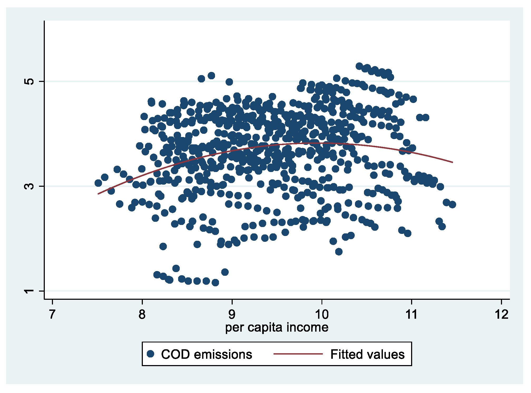It can be found that CO₂ emissions are still growing, but the growth rate has been small since 2011, with an average increase of only 1%, and there was a slight decline in 2015 and 2016. The main element of water pollution is chemical oxygen demand (COD), which has been declining since reaching its peak in 2011. Solid waste emissions have been decreasing since 1998. In fact, solid waste emissions have been eliminated in most provincial regions. In general, although it is impossible to determine whether China’s environmental pollution has declined overall, it can be intuitively judged that the environmental quality has improved significantly. It is more credible to simulate the major pollution emissions and per capita income of the provinces across the country. The quadratic curve simulation diagram of COD, SO₂ and CO₂ emissions and per capita income is attached in the Appendix A. Since solid waste, smoke and dust have already been following an obvious downward trend, they are not listed.

In summary, it seems that the sources of growth have changed in China, while environmental quality has been improved. The previous literature seldom paid attention to the transformation of the sources of growth in China and the theoretical reason for the decrease in environmental pollution caused by this transformation. The “sources of growth” explanation for the EKC put forward by Copeland and Taylor [2] only involves two production factors, physical capital and human capital, but in fact production factors should also include labor and knowledge, so this paper intends to extend the “sources of growth” explanation for the EKC. The second part presents a literature review. In part III, the theoretical mechanism of extending the “sources of growth” explanation for the EKC is analyzed. In the fourth part, the generalized moment estimation (sys-GMM) method is used to conduct empirical research on the panel data of 29 provincial regions in the mainland of China from 1995 to 2017, to analyze whether EKC exists in China and the inflection point appears, whether the production factors of the traditional economy increase the environmental pollution while the production factors of knowledge economy decrease the environmental pollution, whether the sources of growth in China have changed, and whether the economic development stage and environmental pollution are consistent with the “sources of growth” explanation for the EKC. The fifth part concludes and proposes corresponding policy recommendations. Finally, we discuss the limitations of this paper and possible future research directions.

2. Literature Review

Up to present, there is abundant research on the EKC hypothesis, including the confirmation of the existence of the inverted U-shaped curve [5,6], but also studies on the inverted U-shaped curve with insufficient evidence [7], as well as studies of positive N-shaped, inverted N-shaped or other non-linear relationships [8]. Many studies have verified the validity of the EKC hypothesis. These studies have adopted various indicators of energy consumption and environmental quality when investigating whether there is an inverted U-shaped relationship between economic growth and environmental pollution, and included explanatory factors of urbanization, tourism, globalization, trade openness, agriculture, industrialization, globalization, democracy, financial development, etc. [7]. At present, studies applying the four factors of economic growth to environmental pollution to study the EKC hypothesis have not been found. The following literature on the relationship between physical capital, labor, human capital and knowledge, respectively, with environmental pollution provides the research basis for this paper.

On the relationship between physical capital and environmental pollution, most researchers believe that physical capital is the cause of environmental pollution, since capital-intensive industries, usually requiring a large amount of energy input, produce more industrial pollutants and have a greater negative impact on the environment [9,10,11,12,13,14]. Moreover, some studies pointed out that the physical capital invested in clean technology and pollution control, or the physical capital investment under the premise of human capital accumulation, would improve environmental quality. Under reasonable resource and environmental regulations, physical capital investment tends to flow to low-carbon industries, thereby reducing environmental pollution [15,16,17,18,19].

There are few studies on the relationship between labor input and environmental pollution. Most of them believe that labor input will cause environmental pollution because economic growth depending on low-level labor-intensive industries will lead to huge energy consumption and carbon dioxide emission, and will therefore deteriorate the environment [20,21,22,23]. However, compared with physical capital, labor input may have a smaller impact on environmental pollution. It is believed that a labor-intensive production mode may lead to a lower environmental burden than a capital-intensive production mode. Research suggests that capital-saving technological progress has promoted the development of labor-intensive industries, reduced the proportion of capital-intensive industries, and promoted the reduction of smog [13,24,25].

Concerning the research on the relationship between human capital and environmental pollution, most researchers hold that the accumulation of human capital is beneficial to the improvement of environmental quality. Some theoretical research affirms the positive impact of knowledge or human capital on the environment and sustainable development by adding environmental factors to the production function, referring to the human capital spillover model of Lucas [26,27,28] and the knowledge spillover model of Romer [29,30,31]. Grimaud and Tournemaine [32] pointed out that education would reduce pollution under strict environmental policies, using the human capital-driven growth model, and many experiential analyses support this viewpoint [24,33,34,35,36,37,38]. But other empirical studies failed to support the positive significance of human capital on environmental pollution [12,39,40].

As for knowledge, technological innovation or technological progress constitutes an important part thereof. It is generally believed that technological innovation or technological progress is conducive to reducing environmental pollution, but it is also recognized that the “rebound effect” is not conducive to environmental quality. Some studies have classified technology and generally believe that technological progress is of positive significance to environmental governance. Researchers incorporate technological progress into the climate change model and show that technological progress is very important for reducing energy consumption and pollutant emissions, and technological progress is beneficial to the improvement of environmental quality [41,42,43,44,45,46,47,48,49]. But some research found that although the goal of technological progress is to improve energy efficiency and energy conservation, it also triggers an energy rebound effect which is not conducive to the improvement of environmental quality [48,50,51,52,53]. Additionally, there are also researchers who classify technological progress and point out that the environmental effects of different types of technological progress are different, such as capital-intensive technology and labor-intensive technology, or production technology progress and energy-saving technology progress. However, in the long run, technological progress plays an important role in environmental governance [13,25,54].

In general, there is abundant research on the relationship between environmental pollution and the four factors of economic growth, respectively, including physical capital, labor, human capital, and knowledge. However, literature that integrates the four factors of economic growth and environmental pollution to study the EKC hypothesis has not yet been found, so there is no discussion about changes in environmental pollution caused by the transformation of sources of growth. In fact, what is the change in environmental pollution caused by the transformation of sources of growth, and what is the theoretical basis for the changes in environmental pollution? Research on these issues is both innovative and important. This paper intends to follow the “sources of growth” explanation for the EKC [2] and proceed from the four factors of Romer to conduct a further study of the relationship between the sources of growth and environmental pollution, and extend the “sources of growth” explanation for the EKC theoretically and empirically.

3. Theoretical Analysis of Extending the “Sources of Growth” Explanation for the EKC

In this paper, a concise model is applied to describe the “sources of growth” explanation for the EKC. To simplify the analysis, the physical capital is first regarded as the representative production factor of the traditional economy, and human capital as the representative production factor of the knowledge economy. Assuming that a country has two types of industries, one is the dirty industry denoted by M, which is capital-intensive and produces products m and pollutants, while the other is a clean industry denoted by N, which is human-capital-intensive and produces clean products n. Assuming that the technology is given and satisfies the Inada conditions, the reason for the transformation of the economic growth mode is the change in the sources of growth. In the early stage of economic development, physical capital is relatively scarce, and its marginal output is relatively high. Economic growth is mainly driven by physical capital accumulation. With the equalization of factor prices, the scarcity of physical capital and marginal output declined, while the scarcity of human capital and marginal output increased. Then, economic growth started depending mainly on human capital accumulation. The “sources of growth” explanation for the EKC can be proved by the following process.

Referring to Copeland and Taylor [2], express the pollution emissions function as:

$$P=\overline{e}m(\overline{\tau },K_m,H_m)$$

(1)

where P is environmental pollution given endogenously by Formula (1), K is physical capital and H is human capital. $\tau$ is the pollution tax (or the price paid by the company for pollution emissions) and e is the coefficient of pollution emissions. To facilitate the analysis of the impact of changes in K and H on pollution, the pollution tax is assumed to be fixed at $\tau =\overline{\tau }$, and the pollution intensity is assumed to be fixed at $e=\overline{e}$.

The income function can be expressed as:

$$Y=f(K,H,P)$$

(2)

where Y is the total output. If the economic growth is mainly driven by the increase in the accumulation of physical capital K, keeping H unchanged, take the logarithm of Formulas (1) and (2) and then get the differential, respectively:

$$\widehat{P}={\epsilon }_{MK}\widehat{K}$$

(3)

$$\widehat{Y}=s_r\widehat{K}+s_{\tau }\widehat{P}$$

(4)

$\widehat{P}=d\ln (P)=dP/P$, and so on. ${\epsilon }_{MK}$ is the elasticity of the output of industry M relative to the capital factor endowment. According to the Rybczinski theorem, if the quantity of one factor of production increases while the quantity of another factor of production remains unchanged, the number of products produced by an intensive use of the former will increase, while the number of products produced by an intensive use of the latter will decrease. With physical capital increases, products m will increase as physical capital is intensively used in industry M, while clean products produced by industry N, in which human capital is intensively used, will decrease. So there must be ${\epsilon }_{MK}>0$. $s_r$ and $s_{\tau }$ respectively represent the proportion of capital income and pollution tax in total output. $s_r$ > 0. $s_{\tau }$ > 0. By substituting Formula (3) by (4), we can get:

$$\widehat{Y}=(s_r+s_{\tau }{\epsilon }_{MK})\widehat{K}$$

(5)

Since it has been assumed that K increases, namely $\widehat{K}$ > 0, there is $\widehat{P}>0$ and $\widehat{Y}$ > 0. This means that the accumulation of physical capital increases pollution and income at the same time from Formulas (3) and (5).

Similarly, assuming that the economy is mainly driven by the increase in human capital accumulation, keeping K unchanged, then:

$$\widehat{P}={\epsilon }_{MH}\widehat{H}$$

(6)

where ${\epsilon }_{MH}$ is the elasticity of the output of industry M relative to the endowment of human capital. According to the Rybczinski theorem, an increase in human capital accumulation stimulates the output of clean industry N and leads to the decrease of resources of dirty industry M, so there must be ${\epsilon }_{MH}<0$. Furthermore, from Formula (6), we can see that the accumulation of human capital reduces pollution emissions. The impact of increased human capital accumulation on income is:

$$\stackrel{⌢}{Y}=s_w\widehat{H}+s_{\tau }\widehat{P}=(s_w+s_{\tau }{\epsilon }_{MH})\widehat{H}$$

(7)

where $s_w$ > 0 indicates the proportion of human capital income in national income. It has been assumed that H is increasing, that is, $\widehat{H}>0$. And because ${\epsilon }_{MH}<0$, we get $\widehat{P}<0$. Since $s_{\tau }>0$ and ${\epsilon }_{MH}<0$, $s_{\tau }{\epsilon }_{MH}<0$. Since the economic growth is mainly driven by the accumulation of human capital at this time, $s_w$ is relatively large, and the absolute value of the product of $s_{\tau }$ and ${\epsilon }_{MH}$ should be small, that is $s_w>\left|s_w{\epsilon }_{MH}\right|$. Since $\widehat{H}>0$, we get $\widehat{Y}>0$. That is to say, an increase in the supply of human capital while the physical capital remains unchanged will increase national income, which is in line with the general perception. This means, therefore, that the accumulation of human capital promotes income but reduces pollution from Formulas (6) and (7).

We hereby concludes that if the economic growth of a country is mainly driven by the accumulation of physical capital, environmental pollution will increase with the increase of income. And if it mainly depends on the accumulation of human capital in the later stage, environmental pollution will decrease with the increase of income. This is the basic view of the “sources of growth” explanation for the EKC. If labor is the representative production factor of the traditional economy, which means that economic growth is mainly driven by labor-intensive industries, it causes environmental pollution (The existing literature on whether labor input causes environmental pollution has not reached a consensus, but according to the mainstream view and the extensive economic growth model of developing countries, this paper assumes that labor input will probably bring environmental pollution). If knowledge is the representative production factor of the knowledge economy, namely if economic growth is mainly driven by knowledge-intensive industries, there is no environmental pollution. The above-mentioned conclusion of the “sources of growth” explanation for the EKC remains unchanged.

Therefore, when the knowledge economy replaces the traditional economy and the sources of growth change from physical capital and labor to human capital and knowledge, environmental pollution could rise at first and then fall with a sustainable growth in per capita income. It further extended the “sources of growth” explanation for the EKC. To confirm the above point of view, it should first be proven that the main production factors of the traditional economy lead to an increase in environmental pollution, and that the main production factors of the knowledge economy lead to a decline in environmental pollution. Secondly, the existence of the EKC hypothesis should be tested. Finally, according to the economic development stage divided by the sources of growth, it should verify whether the corresponding environmental pollution trend is consistent with the extended “sources of growth” explanation for the EKC.

4. Empirical Analysis of the Relationship between the Sources of Growth and Environmental Pollution

4.1. Econometric Model

Referring to the models of de Mello and Luiz [55] and Ramirez [56], the factor of human capital is put into the production function. The model of de Mello and Luiz [55] involves knowledge stock H, but does not involve labor L. The model of Ramirez [56] involves labor L, but does not involve knowledge stock H. This paper retains the capital K and labor force L of the model of Ramirez and embodies the knowledge stock of the model of de Mello and Luiz as human capital, and the following basic model can be obtained.

$$Y_t=A_t{(\gamma L)}^{\alpha }{K}^{\beta }, \mathrm{in} \mathrm{which} \gamma = H^Z$$

(8)

where Y is the total output represented by the gross regional product, A is technological progress, L is the primary labor input, K is physical capital, $\gamma$ is the human capital coefficient of the primary labor input, H is human capital represented by education level and $z$ is the feedback of education to the original labor input. Here $0<z<1$, $0<a<1$, $0<\beta <1$. Sorting Formula (8), we get:

$$Y_t = (A_t{H}^{z\alpha })(L^{\alpha }{K_d}^{\beta })$$

(9)

Romer divides knowledge into two parts: one is human capital and the other is the technical level [29]. Therefore, in the above formula, AH represents the knowledge economy and LK represents the traditional economy. The human capital H in this paper is measured by the average years of education.

The physical capital of an open economy is composed of domestic capital and foreign direct investment (FDI), which are not homogeneous. The effect of FDI on a country is mainly reflected in its spillover effects, so it should be treated differently [57]. The total physical capital can be defined as the weighted average of domestic capital and FDI, in the mathematical form $K=K_d^{\lambda }FD{I}^{1-\lambda }$. Here, $K_d$ is domestic physical capital, and $\lambda$ is the weight of domestic capital in the total physical capital, $0<\lambda <1$. K is measured by Zhang et al. [58] as reference. Assuming that the initial investment is twice the GDP in 1978, the capital depreciation rate is 7.5%, and the price index of the fixed asset investment is used for the investment price index. The capital calculation formula is $K_{it+1}=(1-\delta )K_{it}+\frac{I_{it+1}}{p_i^K}$, where I is the newly added investment, $p^K$ is the investment price index, i and t are the provinces and time, respectively, and $\delta$ is the depreciation rate. Stock data of FDI are adopted, calculated by the same method as K, and the additional FDI is converted at the average annual exchange rate of RMB to USD in 1995, with a depreciation rate of 7.5% and US consumer price index (CPI). The production function is transformed to:

$$Y_t = A_t{H_t}^{z\alpha }{L_t}^{\alpha }{K_{dt}}^{\beta \lambda }FD{I_t}^{\beta (1-\lambda )}$$

(10)

After taking the natural logarithm of the production function, a linear econometric model is obtained. The variable of environmental pollution P is added as an environmental input (or environmental cost) to the model, and a positive effect on economic growth is expected. This paper takes SO₂ emissions, one of the most representative pollutants of modern civilization, as the indicator of environmental pollution, which is denoted as P_SO₂, and to analyze the robustness of the results, the method of Chen [4] is used to calculate CO₂ emissions based on the consumption of fossil energy including coal, oil and natural gas, denoted as P_CO₂. Moreover, the method of Tan and Wen [59], which compiled the prices required to restore the environmental impact of major pollutants such as CO₂, SO₂, COD, smoke and dust, is used to calculate the comprehensive environmental pollution loss, denoted as P_pul. As for the variable of knowledge, some studies regard the number of patents as the indicator, but this paper believes that it cannot reflect the actual knowledge innovation because the number of patents is not equivalent to the quality of patents. This paper intends to measure knowledge from the perspective of the result of the promotion of economic growth and environmental protection. Since a significant feature of the knowledge economy is sustainable economic development, this paper adopts the green technological progress rate, GTP, as the main indicator of the knowledge economy, and it is expected to be positive on economic growth and negative on environmental pollution. Referring to Jing and Zhang [60], green technological progress is measured by green total factor productivity. This paper used the directional distance function (DDF) and the fixed reference Malmquist model to calculate the green total factor productivity from 1996 to 2017, setting the green technological progress in 1995 to 1. The input variables include the capital stock, total number of employees and total energy consumption. The expected output is the GDP of each region at constant prices in 1995, and the undesired output includes CO₂, COD and SO₂ emissions. And the index of green technological progress is obtained by the cumulative multiplication method of Qiu [61]. The variable of R&D is further introduced to observe the impact of innovation, since the efficiency of R&D determines its economic effects and the direction of R&D determines the environmental effects. For the R&D indicator, the R&D investment of each province was converted to a constant price in 1995 by CPI and divided by GDP to get the “R&D investment of 10,000 yuan GDP”. Due to the large economic gap between the eastern, middle and western regions of China, the control variable of location, Loc, is added to the model. Loc has three numbers: 1 represents the eastern region, 2 represents the central region and 3 represents the western region. The following linear econometric model is obtained:

$$\begin{array}{ll}\ln {(Y)}_{it}=& {\alpha }_0+{\alpha }_1\ln {(K)}_{it}+{\alpha }_2\ln {(L)}_{it}+{\alpha }_3\ln {(H)}_{it}+{\alpha }_4\ln {(FDI)}_{it}+{\alpha }_5\ln {(P)}_{it}+{\alpha }_6\ln {(R\&D)}_{it}\hfill \\ & +{\alpha }_{7}GT{P}_{it}+{\alpha }_{8}Loc+e_{it}\hfill \end{array}$$

(11)

To confirm the extended “sources of growth” explanation for the EKC proposed previously, P is set as the explained variable. And according to the general model of the EKC hypothesis, the explanatory variables of output are set as per capita income y and y². Thus, the following linear econometric model is obtained:

$$\begin{array}{ll}\ln {(P)}_{it}=& {\alpha }_0+{\alpha }_1\ln {(y)}_{it}+{\alpha }_2\ln {{(y)}^2}_{it}+{\alpha }_3\ln {(K)}_{it}+{\alpha }_4\ln {(L)}_{it}+{\alpha }_5\ln {(H)}_{it}+{\alpha }_6\ln {(FDI)}_{it}\hfill \\ & +{\alpha }_7\ln {(R\&D)}_{it}+{\alpha }_{8}GT{P}_{it}+{\alpha }_{9}Loc+e_{it}\hfill \end{array}$$

(12)

4.2. Data Description

All the variables range from 1995 to 2017. All price data are based on 1995. Due to data availability, they include 29 provincial regions in the mainland of China, excluding Tibet and Chongqing. Data are taken from China’s Energy Statistics Yearbook, China’s Population and Employment Statistics Yearbook, China’s Statistical Yearbook on Environment, China’s Statistical Yearbook on Science and Technology and China’s Statistical Yearbooks of provinces.

The descriptive statistics of the natural logarithm of variables are listed in

Table 1. Descriptive statistics of variables.

Variables	Mean Value	Median Value	Standard Deviation	Minimum Value	Maximum Value	Number of Observations
LnYit	8.400	8.469	1.152	5.123	10.97	667
Lnyit	9.679	9.760	0.924	6.430	11.650	667
LnKit	9.470	9.447	1.124	6.354	11.97	667
LnFDIit	6.017	6.149	1.727	−3.042	9.098	667
LnLit	7.525	7.634	0.839	5.483	8.820	667
LnHit	2.090	2.101	0.149	1.546	2.526	667
LnR&Dit	−0.148	−0.140	0.874	−3.760	2.130	667
GTPit	4.232	2.460	4.963	0.892	73.86	667
LnP_SO2it	3.887	4.030	0.976	0.360	5.450	667
LnP_CO2it	9.697	9.760	0.924	6.430	11.65	667
LnP_pulit	5.271	5.354	1.010	1.744	7.412	667

.

4.3. Empirical Analysis

4.3.1. Estimation Method

In Formulas (12) and (11), there may be bidirectional interactive relationships between the explained variables and explanatory variables such as Y and P, which leads to the endogenous problems. To obtain an unbiased estimate, Arellano and Bond [62] proposed the first differenced GMM estimation, but Blundell and Bond [63] pointed out that because the lag value of a variable is not an ideal instrument of the first-order difference equation, the first differenced GMM might be influenced by weak instrumental variables and got biased estimation results. So, Arellano and Bover [64] and Blundell and Bond [63] proposed a more effective method of system GMM. Sys-GMM includes a one-step and two-step method. Arellano and Bond [62] indicated that the two-step method is more reliable than the one-step method through Monte Carlo simulation. Roodman [65,66] further discussed how to implement the differenced and system GMM in Stata. Based on it, the estimation method used in this study is the two-step system Generalized Method of Moment.

The applicability of this method can be explained through the following four aspects. First, the number of cross-sections (n = 29) is greater than the number of time series (t = 23), which meets the benchmark requirements for implementing GMM. Second, the dependent variable is continuous. The correlation coefficients between the regional GDP, P_SO₂, P_CO₂, P_pul and their first-order lag are 0.998, 0.999, 0.986 and 0.985, respectively—higher than 0.800, the threshold required to establish continuity. Third, the GMM technology using panel data will not eliminate inter-provincial changes, and the control variables of location were set in the econometric model to test the impact of inter-provincial differences, which largely compensates for the adverse effects of the potential spatial autocorrelation on the model. Fourth, the estimation strategy takes endogeneity into account by accounting for simultaneity in the explanatory variables through an instrumentation process, on the one hand, and controlling for the unobserved heterogeneity with time-invariant indicators, on the other hand. Fifth, the two-step method is chosen because it controls for heteroscedasticity, whereas the one-step method only controls for homoscedasticity [67].

This paper pays special attention to the possible multicollinearity. First, this paper uses Stata14 for panel data testing. Strictly collinear variables will be automatically eliminated by Stata [68]. Second, the calculated value of variance inflation factors (VIF) between the explanatory variables of Formula (11) are all less than 10, and the mean VIFs of the model with P_pul, P_SO₂ and P_CO₂ as explanatory variables are 5.12, 4.62 and 4.3, respectively. Therefore, it can be judged that the model does not have serious multicollinearity problems. By calculating the variance inflation factors between the explanatory variables of Formula (12), it is found that the mean VIF of the model was greater than 100, since the VIFs of y and y² were, respectively, 582.78 and 581.81. The preliminary judgment is that there is a serious multicollinearity. Moreover, the mean VIF drops to 7.74 after removing y² from the model, and then the serious multicollinearity can be eliminated. However, in this case, the model cannot test the inverted U-shaped impact of per capita income y on environmental pollution P, and the models commonly used in academia regarding the EKC hypothesis cannot be applied either. Since Grossman and Krueger [3] first proposed the EKC hypothesis and its model, there have been a lot of papers following this research around the world. The model generally contains explanatory variables y and y², or even y³ [3,6,7,8,69]. Such model settings tend to produce serious multicollinearity. Woodridge [70] proposed that some variables can be removed in order to eliminate multicollinearity, but unfortunately this may lead to bias estimation. He believes that the high VIF cannot really affect our decision. Third, from the test results in

Table 2. System Generalized Method of Moment (Sys-GMM) estimation results (the explained variable is Y).

Explanatory Variables	The Explanatory Variable of P_SO2	The Explanatory Variable of P_CO2	The Explanatory Variable of P_pul
LnHit	1.1854 ***	1.3266 ***	1.2217 ***
	(10.88)	(10.04)	(12.33)
LnLit	0.2588 ***	0.3977 ***	0.2356 ***
	(8.79)	(11.51)	(7.63)
LnKit	0.6464 ***	0.3877 ***	0.1562 ***
	(23.80)	(14.27)	(3.83)
LnGTPit	0.0182 ***	0.0059 ***	0.0025 ***
	(17.82)	(10.87)	(4.73)
LnFDIit	0.0043	0.0752 **	0.1878 ***
	(0.10)	(2.56)	(5.23)
LnPit	0.2748 ***	0.3231 ***	0.5871 ***
	(17.41)	(15.98)	(11.00)
LnR&Dit-1	−0.0574 ***	−0.0268 ***	−0.0618 ***
	(−3.58)	(−3.98)	(−5.55)
Loc	−0.1608 ***	−0.0474	−0.0309
	(−3.12)	(−1.05)	(−0.61)
Constant term	−3.0004 ***	−4.5542 ***	−1.6137 ***
	(−12.55)	(−11.63)	(−4.69)
Wald test	81,935.74 (0.000)	506,704.91 (0.000)	43,143.14 (0.000)
AR (2) test	0.73 (0.465)	0.69 (0.490)	0.59 (0.555)
Hansen test	27.59 (0.119)	27.00 (0.135)	23.76 (0.253)
DHT for instruments (a) GMM instruments for levels H excluding group Dif (null H = exogenous)	0.793	0.735	0.162
(b) IV (Years, eq (diff)) H excluding group Dif (null H = exogenous)	0.811	0.878	0.393
Number of Instruments	29	29	29
Number of Provinces	29	29	29
obs	580	580	580

Note: ***, ** represent the significance level of 1% and 5% respectively. The coefficients in parentheses of variables and constant terms are z values. The coefficients in parentheses of the Wald test, the Hansen test and the AR(2) test are p values.

and

Table 3. Sys-GMM estimation results (the explained variable is P).

Explanatory Variables	The Explained Variable of P_SO2	The Explained Variable of P_CO2	The Explained Variable of P_pul
Lnyit	3.4264 ***	2.6950 ***	3.2314 ***
	(3.02)	(3.67)	(6.36)
Lny2it	−0.1794 ***	−0.1293 ***	−0.1572 ***
	(−2.71)	(−2.90)	(−5.51)
LnHit	−0.8132 **	−0.8350 ***	−0.6243 ***
	(−2.13)	(−3.49)	(−6.71)
LnLit	0.7552 ***	0.4053 **	0.3954 ***
	(2.79)	(2.43)	(5.85)
LnFDIit	0.7006 ***	0.1296 ***	−0.0179
	(9.69)	(2.79)	(−0.57)
LnKit	−0.2457	0.3703 **	0.5318 ***
	(−0.85)	(2.34)	(6.10)
LnR&Dit	0.0638	0.0456	0.0758 ***
	(1.10)	(1.16)	(2.76)
GTPit	−0.0927 ***	−0.0136 ***	−0.0005
	(−7.79)	(−3.08)	(−0.28)
Loc	0.9767 ***	0.3133 **	0.2113 ***
	(6.51)	(2.46)	(3.66)
Constant term	−19.8062 ***	−10.3379 ***	−18.1128 ***
	(−4.23)	(−3.70)	(−8.16)
Wald test	1034.27 (0.000)	2080.46 (0.000)	88,742.11 (0.000)
AR(2) test	1.64 (0.101)	1.04 (0.299)	1.30 (0.193)
Hansen test	17.96 (0.117)	20.41 (0.202)	27.59 (0.278)
DHT for instruments (a) GMM instruments for levels H excluding group Dif (null H = exogenous)	0. 253	0. 879	0. 994
(b) IV (Years, eq (diff)) H excluding group Dif (null H = exogenous)	0. 349	0. 980	0. 997
Number of Instruments	22	26	34
Number of Provinces	29	29	29
obs	609	609	609

Note: ***, ** represent the significance level of 1% and 5% respectively. The coefficients in parentheses of variables and constant terms are z values. The coefficients in parentheses of the Wald test, the Hansen test and the AR (2) test are p values.

, it is found that t-tests of the core variables are significant and in line with economic expectations. Chen [68] believes that if multicollinearity affects the significance of the core variables, it should be dealt with. But if multicollinearity does not affect the significance of the core variables, it is not necessary to deal with it, because if there is no multicollinearity, the coefficient of the variable will only be more significant.

4.3.2. The Estimated Result and Robustness Test of Output as the Explained Variable

To verify whether the sources of growth in China have changed, the econometric model of Formula (11) is tested, and the estimation results are shown in Table 2. For the three equations, the Wald coefficients are significant. The AR (2) test shows that there is no second-order serial correlation in the disturbance term. p values of the Hansen test are greater than the significance level of 0.1, indicating that there is no over-identification of instrumental variables. The DHT test consists of two parts: one is to test (a) whether the instrumental variable in GMM brackets is exogenous, and the other is to test (b) whether the instrumental variable in IV brackets is exogenous, and its null hypothesis is that the instrumental variable is exogenous. P values of the DHT test are all greater than the significance level of 0.1, indicating that the instrumental variables are exogenous.

According to the estimated results, human capital has become the primary factor to promote China’s economic growth, and the coefficient is significantly larger than other factors, followed by physical capital, environmental pollution and labor, and finally green technological progress and FDI. Their role in promoting economic growth decreases in turn. The coefficient of human capital is significantly positive and the largest. This is firstly due to the rapid accumulation of human capital in China in recent years (refer to the second paragraph of this paper); secondly, the accumulation of human capital in China coincides with a large-scale industrial transformation and upgrading; thirdly, the growth rate of the production factors of traditional economic growth, such as physical capital and labor, has slowed. This is consistent with the research conclusion of Jian et al. [71] on China’s human capital. The coefficient of physical capital is significantly positive but less than that of the human capital. On the one hand, it shows that China still has large investment demand, which has driven large-scale investment and economic growth; on the other hand, it also shows that under the background of China’s large-scale industrial transformation and upgrading, the dependence of economic growth on the amount of investment has declined, and more depends on the quality of investment, and the improvement of investment quality actually depends on the accumulation of human capital. The coefficient of labor force is significantly positive. At present, China is still the most populous country, so the labor force still plays a huge role in economic growth. However, due to the declining population growth rate in China, the demographic dividend has gradually declined. Economic growth no longer depends on the quantity of primary labor input, but on the quality of labor input, that is, the level of human capital. The coefficient of environmental pollution is significantly positive. The current economic growth in China is still relatively extensive, so environmental pollution has brought economic growth as a cost. The coefficient of green technological progress is significantly positive. China’s industrial transformation and upgrading is accelerating, and environmental regulations have been increasingly strengthened. Moreover, after passing a certain turning point, they have promoted the green technological progress [72]. The progress of green technology has also promoted the development of green industries and a green economy. This result is exciting, which means that sustainable economic growth could be achieved. The coefficient of FDI is significantly positive, but small. On the one hand, a large scale of FDI flows into China every year, which is still one of the driving forces of economic growth in China; but, on the other hand, due to China’s growing economy, the ratio of FDI to domestic investment is declining, and thus the effect of driving economic growth is smaller. R&D has a small but negative effect on economic growth, which is consistent with the research of Song et al. [73]. This may be due to the low efficiency of current R&D, and the substantial increase in R&D expenditure has offset the positive effect on economic growth. In general, human capital and green technological progress in the knowledge economy have become important factors that promote economic growth at present.

Given the increasing role of the knowledge economy, according to the extended “sources of growth” explanation for the EKC—if the EKC exists—the current stage of environmental pollution should be near the inflection point, or have passed the inflection point. Since the previous paper has proved that China has passed the inflection point from the national average level, the trend of China’s environmental pollution and the stage of economic transformation and development are consistent with the extended “sources of growth” explanation for the EKC, that is, the theoretical hypothesis has been verified.

4.3.3. Analysis of Estimation Results and Robustness Test of Environmental Pollution as the Explained Variable

To verify whether the EKC exists under the change of sources of growth in China and whether the inflection point of per capita income has appeared, the econometric model of Formula (12) is tested by panel data, and three different pollution indicators are used as the explained variables, respectively, for the robustness test. The estimation results are shown in Table 3. From the results, we can see that the Wald coefficients are significant. The AR (2) test results show that there is no second-order serial correlation in the disturbance term. The p values of the Hansen test are greater than the significance level of 0.1, indicating that there is no over-identification of instrumental variables. The p values of the DHT test are all greater than the significance level of 0.1, indicating that the instrumental variables are exogenous.

The estimation results show that the variables of per capita income, labor force, domestic physical capital, FDI and R&D have a positive impact on environmental pollution, and the variables of per capita income, labor input and domestic physical capital have a particularly significant impact on the pollution losses. The coefficient of per capita income is significantly positive and the largest in the three measurement results, indicating that economic growth is the most important cause of environmental pollution, and the square of per capita income is significantly negative, showing the inverted U-shaped relationship between environmental pollution and per capita income, which confirms the EKC hypothesis. The inflection points of the three equations were calculated as 9.5496, 10.4215 and 10.2780 respectively. According to the data of per capita income for the base period in 1995, this factor has exceeded the inflection point of the first equation, with P_SO₂ as the explained variable in 29 provincial regions, and exceeded the inflection point of the second equation, with P_CO₂ as the explained variable in 13 provincial regions, as well as that of the third equation, with P_pul as the explained variable in 16 provincial regions. The above inflection points are all lower than the average value of 10.4549 in each province in 2017, indicating that the inflection point has been exceeded from the national average level. The coefficient of the labor force is significantly positive, which indicates that the extensive labor-intensive production mode still exists in China. Increasing labor input means the increase of environmental pollution. The coefficient of domestic physical capital is significantly positive, indicating that the physical capital investment in China is still accompanied by a large number of natural resources and energy investment, and the increase in physical capital investment has led to an increase in environmental pollution. In the third equation, it is found that FDI promotes environmental pollution, which is consistent with the research on China of Yi et al. [13], who confirmed the Pollution Paradise hypothesis. It shows that the introduction of FDI in China may not be environmentally friendly, or the spillover of FDI technology has not improved environmental pollution well, and the spillover effect of environmental protection technology is not enough. The coefficient of R&D is significantly positive, which may due to the fact that, under the background of the current extensive economic development, the technological progress bias pollution and the lack of green technology research and development led to an increase in environmental pollution, with research and development increasing.

Human capital level and green technological progress have a negative impact on environmental pollution, which is consistent with the research of Li et al. [69]. The level of human capital has the greatest impact on environmental pollution. This is because education is one of the main sources of knowledge and modern technology, an important foundation for improving the concept of green development and an important prerequisite for the transformation of the intensive production mode and for innovation and management. In the third equation, green technological progress is negatively correlated with environmental pollution. This is because green technological progress is beneficial to the economy, developing toward intensification and low carbon, and getting the same economic output with less material resources and environmental pollution.

To sum up, the production factors of physical capital and labor force of the traditional economy have contributed to the increase of environmental pollution, while the production factors of human capital and the green technological progress of the knowledge economy have promoted the decline of environmental pollution. EKC exists in China, and environmental pollution has basically passed the turning point at this stage. Therefore, the trend of China’s environmental pollution and the development stage of economic transformation are consistent with the “sources of growth” explanation for the EKC, that is, the theoretical hypothesis has been verified.

5. Conclusions and Policy Implications

From the perspective of Romer’s four factors of economic growth, this paper discusses the extended “sources of growth” explanation for the EKC and adopts the sys-GMM to conduct an empirical analysis of panel data from 29 provinces in the mainland of China. On the whole, the test results support the theoretical hypothesis proposed in this paper. The main conclusions and policy suggestions are as follows:

First, the EKC hypothesis exists in China, since that there is a trend according to which environmental pollution increases first and then decreases. Furthermore, China is passing through the EKC inflection point. It has passed the EKC inflection point for SO₂ emissions in all of the 29 provincial regions in the mainland of China, and for CO₂ and comprehensive environmental pollution losses in 13 and 16 provincial regions, respectively. The above inflection points are all lower than the average value of 10.4549 for per capita income of each province in 2017, indicating that the inflection point has generally been passed from the national average level.

This suggests that China should strengthen its environmental regulations to improve environmental quality and avoid pollution first and then treatment. Environmental regulations are conducive to improving environmental quality [1], and to achieve continuous environmental improvement China should take the initiative to strengthen environmental regulations and improve environmental quality, rather than believing in the EKC hypothesis, according to which environmental pollution will automatically decrease after the economic development reaches a certain level. Specific measures include: (1) utilizing the environmental clauses of free trade agreements to promote the improvement of environmental policies and regulations; (2) taking advantage of the technical mechanisms of the United Nations Framework Convention on Climate Change to promote technological progress, especially the development of environmental protection technologies; (3) implementing industrial policies and tax policies that are conducive to environmental protection; (4) promoting environmental protection awareness and strictly enforcing environmental protection laws.

Second, the production factors of the traditional economy, physical capital and labor input, are positively related to environmental pollution, while the production factors of the knowledge economy, human capital and green technological progress, are negatively related to environmental pollution.

This suggests that physical capital investment should be actively encouraged, to invest in clean industries such as high-tech industries, environmental protection industries and tertiary industries, as well as in rural areas and agriculture, to promote rural revitalization. In terms of labor, China should gradually restrict the development of polluting labor-intensive industries, promote the development of tertiary industries with stronger employment absorption capabilities, especially the producer service industries, and appropriately encourage the development of green and environmentally friendly traditional handicraft industries. For human capital, China should continue to increase the education funding input and improve the quality of education to increase human capital accumulation, strengthen the awareness of environmental protection in basic education, promote the development of environmental protection courses in professional education and encourage the establishment of environmental-protection-related majors and the development of environmental-protection-related degrees at all levels. Moreover, in terms of knowledge, it is necessary to encourage R&D personnel and funds to green technology. National and local technology award policies should be beneficial to green technology development.

Third, China is in the process of transforming the traditional economy into a knowledge economy, and the production factors of the knowledge economy have become important in promoting sustainable economic growth in China. The current stage of China’s economic growth and environmental pollution trends are consistent with the extended “sources of growth” explanation for the EKC.

This shows that it is necessary to follow the path of coordinated development of economic growth and environmental protection. The transformation of the sources of growth promotes a sustainable economic development in China, as well as leading to a downward trend in environmental pollution. Therefore, the sources of growth should be guided from physical capital and labor to human capital and knowledge, to promote an intensive economic growth and sustainable development.

6. Discussion

Previous research has studied the relationship between Romer’s four factors of economic growth and environmental pollution. This paper integrates them into a unified theoretical framework. It finds that the sources of growth have changed from physical capital and labor to human capital and knowledge in China, transformed from a traditional economy into a knowledge economy. Then, using Chinese provincial data by sys-GMM, this paper verified that the transformation brought about environmental pollution, first increasing and then decreasing, which extended the “sources of growth” explanation for the EKC. This new work not only strengthens the theoretical applicability of the EKC hypothesis but also has an important significance for China, as well as for other similar nations, which can also implement a sustainable development of coordinated economic growth and environmental protection.

Due to the importance of green sustainable development [74,75], the theoretical viewpoint of this paper needs more evidence. First, we believe that using the data of smoke, dust, COD and other pollutant emissions that have been significantly reduced is of little empirical significance, but it is necessary for China to use more environmental data, including ecological footprints, to conduct further research. Additionally, the lack of industry data in China and samples of other nations limits the research conclusions. Further research will be of great significance to enrich the theory of sustainable economic development. Besides, this paper does not analyze the transformation mechanism of the sources of growth under environmental regulations, which can be further studied in the future.