Article

Environmental Regulation, Resource Misallocation and Industrial Total Factor Productivity: A Spatial Empirical Study Based on China’s Provincial Panel Data

1
School of Economics, Zhengzhou University of Aeronautics, Zhengzhou 450046, China
2
School of Information Management, Zhengzhou University of Aeronautics, Zhengzhou 450046, China
3
School of Economics and Business Administration, Central China Normal University, Wuhan 430079, China
*
Author to whom correspondence should be addressed.
Sustainability 2021, 13(4), 2390; https://doi.org/10.3390/su13042390
Submission received: 8 January 2021 / Revised: 18 February 2021 / Accepted: 19 February 2021 / Published: 23 February 2021

Abstract

:
A vast theoretical and empirical literature has been devoted to exploring the relationship between environmental regulation and total factor productivity (TFP), but no consensus has been reached and the reason may be attributed to the fact that the resource reallocation effect of environmental regulation is ignored. In this paper, we introduce resource misallocation in the process of discussing the impact of environmental regulation on TFP, taking China’s provincial industrial panel data from 1997 to 2017 as a sample, and the spatial econometric method is employed to investigate whether environmental regulation has a resource reallocation effect and affects TFP. The results indicate that there is a U-shaped relationship between environmental regulation and industrial TFP and a negative spatial spillover effect of environmental regulation on industrial TFP at the provincial level in China. Both capital misallocation and labor misallocation will lead to the loss of industrial TFP. Capital misallocation has a negative spatial spillover effect on industrial TFP, while labor misallocation is just the opposite. Environmental regulation can produce a positive resource reallocation effect, which in turn promotes the industrial TFP in the range of 28% to 33%, while capital misallocation and labor misallocation are only partial mediator.

1. Introduction

Total factor productivity (TFP) is an important indicator to measure the quality of economic development. The development history of the world’s major developed countries shows that TFP has become increasingly important to the sustainable economic growth with the succession of development stages. The 19th National Congress of the Communist Party of China (CPC) held that “China’s economy has been transitioning from a phase of rapid growth to a stage of high-quality development” and that we must “work hard for better quality, higher efficiency, and more robust drivers of economic growth through reform and raise TFP.” Industry plays a pivotal role in the national economy. Improving the quality of industrial development is crucial to China’s overall economic development in the future. Generally, there are two ways to promote TFP: one is to improve production efficiency through technological progress; the other is to improve allocation efficiency through resource optimization and reorganization. Since it is difficult to achieve major breakthroughs in technological innovation in short term, it is important to seek TFP improvement through resource reallocation. However, due to the inadequate development of market economy, different degree of market distortions and resource misallocation can be widely observed in the industrial field of China’s economy, which not only hinders the improvement of industrial TFP, and also aggravate the degree of regional industrial development imbalance.
Although China’s industrial development achievements have attracted worldwide attention since the reform and opening up, but the extensive growth model driven by various factors has led to great damage to ecological environment. In recent years, with the increasing severe resource and environmental problems, environmental regulation has become an important policy instrument for government to deal with environmental problems and improve the quality of development. As the main source of environmental pollution, the government has attached great significance to the environmental regulation in the industrial field. A large number of studies have shown that environmental regulation will directly affect TFP, but the conclusions are different. One of the important reasons is that the impact of environmental regulation is likely to produce asymmetry in the face of heterogeneous enterprises or spatial units and this asymmetric rule may produce resource reallocation effects. Therefore, if we pay attention to the impact of environmental regulation on TFP, we must not ignore its possible reallocation effects.
Theoretically, the strength of environmental regulation and degree of resource misallocation in different regions will not only affect their own TFP, but also affect other regions through spatial spillover effects because of spatial heterogeneity and spatial dependence. Meanwhile, different environmental regulation levels may induce the cross-regional flow of resources, which has an impact on resource allocation among regions. So, for China’s industry, what is the impact of environmental regulation and resource misallocation on TFP? How much the spatial spillover effect of them on regional TFP? Will environmental regulation improve the resource misallocation among regions? How does it affect industrial TFP by acting on resource misallocation? These are theoretical and practical issues worthy of in-depth discussion, which also constitute the aim and purpose of this paper.

2. Literature Review

Up to now, research on the relationship between environmental regulation and TFP can be summarized as the verification of three hypotheses [1], but conclusions are still controversial. The first is restriction hypothesis, which holds that environmental regulation will lead to a rise in production costs and a crowding-out effect on investment, thus damaging the TFP and competitiveness of enterprises based on the neoclassical framework [2,3,4,5,6], and this constraint effect will be gradually transmitted to industrial level and regional level. The second is the Porter hypothesis, whose main point is that well-designed environmental regulation can encourage enterprises to improve their technological level, partially or even completely offset the increase in costs caused by environmental regulation, so as to improve TFP of enterprises, industries and macro-economy [7,8,9,10,11,12]. The last is uncertainty hypothesis, and its core view is that the impact of environment regulation on TFP is uncertain [13,14]. This uncertainty is manifested in two aspects: (i) The relationship between environmental regulation and TFP shows nonlinear characteristics such as U-shaped [15,16], inverted U-shaped [17,18,19,20], inverted N-shaped [21,22] and J-shaped [23]. (ii) For heterogeneous regulatory types [24,25], industries [26,27] and regions [28], the impact of environmental regulation on TFP is significantly different.
As the most major developed economies in the world, how to deal with the relationship between environmental protection and economic development in the US, EU and Japan has received continuous attention from the academic circle, and the research on their environmental regulation and TFP has emerged in endlessly. Although part of the literature has taken these regions as samples when we reviewed the three hypotheses, the main research viewpoints have not been listed. Different from the Chinese scholars’ focus on the impact of environmental regulation on TFP of medium-sized industries or macro-regions, the relevant studies on the EU, Japan and US pay more attention to the relationship between environmental regulation and TFP at the micro-enterprise level. Taking manufacturing enterprises as the main research object, most of the research conclusions are deterministic, which confirms the restriction hypothesis or the Porter hypothesis [29,30,31,32,33].
Resource misallocation may lead to TFP loss and inter-departmental differences, which has basically formed a consensus in academic circles, but the train of thought of theoretical analysis is different. One way is called “direct method,” which chooses several factors that are considered important in theory and experience, and tries to directly quantify the degree of resource misallocation and TFP loss caused by these factors. Researchers mainly examine them from the perspectives of policy distortion [34,35,36,37] and institutional distortion [38,39]. The other way is called “indirect method,” which analyzes all potential factors that may lead to resource misallocation and quantifies its impact on TFP by building a theoretical model. Researchers generally examine how TFP changes with the resource misallocation parameter faced by enterprises [40]. Hsieh and Klenow (2009) made a pioneering contribution to this [41]. Starting from resource misallocation at the enterprise level, they established a theoretical framework from micro to macro based on the degree of TFP dispersion, and quantified its impact on aggregate TFP. Many scholars have followed their idea to improve the theoretical framework of the impact of resource misallocation on TFP after that [42,43,44].
As for the relationship between environmental regulation and resource misallocation, it essentially stems from the discussion about restriction hypothesis and Porter hypothesis of environmental regulation. The reason why the two hypotheses about the effect of environmental regulation on TFP are opposite, is the ignorance of the resource reallocation effect of environmental regulation, in addition to sample selection, measurement errors and other factors [29]. In fact, due to the existence of heterogeneity, environmental regulation is easy to produce asymmetry in the process of enterprise decision-making, and this asymmetry is very likely to result in resource reallocation effect. As a pioneering literature on the relationship between environmental regulation and resource misallocation, Tombe and Winter (2015) pointed out that environmental regulation based on pollution intensity may form a “wedge” that lead to resource misallocation in the factor market equilibrium, which has an impact on aggregate TFP [45]. However, their research does not seem to be suitable for China, and the root cause lies in the different backgrounds of the implementation of China’s environmental policies. The existing research on the relationship between environmental regulation and resource misallocation in China focuses on the resource reallocation effect of binding pollution control environmental regulation [46]. Unfortunately, the research in this field has just started, and both theoretical explanation and empirical evidence are not enough.
However, few literatures have comprehensively analyzed the relationship between environmental regulation, resource misallocation and TFP, and no literature has investigated the spillover effects of environmental regulation, resource misallocation on TFP and how environmental regulation affects TFP through resource misallocation under the conditions of spatial heterogeneity and spatial dependence [47]. In this context, we will take the Chinese provincial panel data as a sample and use the spatial econometric methods to investigate the direct effect and spatial spillover effect of environmental regulation and resource misallocation on industrial TFP, and the mechanism of environmental regulation affecting industrial TFP via resource misallocation.

3. Research Hypotheses

3.1. Environmental Regulation and TFP

From a large number of studies on the relationship between environmental regulation and TFP, the restriction hypothesis, Porter hypothesis and uncertainty hypothesis all take enterprise as the starting point of theoretical analysis, and draw different conclusions that environmental regulation affects TFP. Similarly, we can also regard “spatial unit” as specific actors, and when they are faced with environmental regulation, like enterprises, their TFP must be affected to a certain extent. In the following discussions, we regard each province as a decision-making unit, and industrial TFP is calculated according to the aggregate input and output, which is mainly due to the incomplete statistics of industrial sub-sectors at the provincial level. Before empirical test, we cannot judge whether the impact of environmental regulation on TFP is positive or negative, but according to the CGE (computable general equilibrium) theory simulation proposed by Li et al. (2012), environmental regulation has a higher probability that it will lead to regional TFP losses [48]. Moreover, local governments in different regions may lead to competition in environmental regulation due to different environmental protection situations, which makes environmental regulation have a spatial spillover effect on TFP. It should be noted that the environmental regulation of a region is usually not strengthened indefinitely [49], and it is difficult for the environmental performance caused by overly stringent environmental regulation to make up for the loss of economic performance. Accordingly, we put forward the following hypotheses:
Hypotheses 1a (H1a).
The strengthening of environmental regulation will directly lead to the decline of regional industrial TFP.
Hypotheses 1b (H1b).
There is a strong spatial spillover effect of environmental regulation on industrial TFP.
Hypotheses 1c (H1c).
The direct impact and spillover effect of environmental regulation on regional industrial TFP may be non-linear with the increase of regulation intensity.

3.2. Resource Misallocation and TFP

A large number of studies have proved that resource misallocation will lead to TFP loss. At the region-level, if there exists serious resource misallocation in a specific region, its industrial TFP will inevitably be negatively affected. Because of the resource mobility among regions, resource misallocation in a region usually means the allocation of resources in the neighborhood cannot meet the optimization conditions of equal marginal revenue, which leads to resource misallocation and TFP loss in the neighborhood. Accordingly, we put forward the following hypotheses:
Hypotheses 2a (H2a).
Resource misallocation will lead to the decline of regional industrial TFP.
Hypotheses 2b (H2b).
Resource misallocation has negative spatial spillover effect on regional industrial TFP.

3.3. Environmental Regulation, Resource Misallocation and TFP

According to Tombe and Winter (2015), environmental regulation may produce a “wedge” that leads to resource misallocation in the equilibrium of factor market, which in turn has an impact on TFP [45]. In other words, resource misallocation can be regarded as a transmission path for environmental regulation to affect industrial TFP. In view of the differences in environmental regulation intensity in different regions, the factors of production in areas with higher intensity of regulation tend to flow to areas with lower intensity of regulation for profit, but how the resource allocation of the relevant areas will change is uncertain, which mainly depends on their initial state of resource allocation. On the one hand, environmental regulation may optimize resource allocation; on the other hand, it may also aggravate the resource misallocation. If environmental regulation helps to improve the resource allocation, the impact of environmental regulation on regional industrial TFP has a positive resource reallocation effect; on the contrary, the impact of environmental regulation on regional industrial TFP has a negative resource reallocation effect. On the basis of this, we put forward the following two opposite hypotheses:
Hypotheses 3a (H3a).
Environmental regulation is helpful to alleviate resource allocation and thus improve regional industrial TFP.
Hypotheses 3b (H3b).
Environmental regulation will aggravate resource misallocation and lead to the decline of regional industrial TFP.

4. Model Specification and Data Source

4.1. Model Specification

In order to verify Hypotheses H1a, H1b and H1c, the spatial durbin model (SDM), which includes both dependent variable spatial lag and independent variables spatial lag, is used as the benchmark model for spatial interaction analysis [50,51], i.e.,
T F P i t = α + ρ W T F P j t + β 1 E R i t + β 2 E R i t 2 + γ X i t +   θ 1 W E R j t + θ 2 W E R j t 2 + η W X j t + μ i + λ t + ε i t
where T F P i t is the industrial TFP level of the i t h province in year t ; E R i t is the environmental regulation intensity of the i t h province in the t t h year, and E R i t 2 is the square of environmental regulation. X denotes a vector consisting of a series of control variables. μ i , λ t and ε i t represent the provincial fixed effect, year fixed effect and random disturbance, respectively. W is a spatial weight matrix, which is constructed based on queen adjacency. If province i and province j have a common boundary or vertex, the element w i j   =   1 in matrix W ; otherwise, w i j   =   0 .
In order to verify Hypotheses H2a and H2b, we set model (2) by imitating Equation (1).
T F P i t = α + ρ W T F P j t + β 1 M i s K i t + β 2 M i s L i t + γ X i t +   θ 1 W M i s K j t + θ 2 W M i s L i t + η W X j t + μ i + λ t + ε i t
where M i s K i t and M i s L i t are the degree of capital and labor misallocation of the i t h province in year t , respectively. The meanings of other variables and symbols are the same as above.
In order to verify Hypotheses H3a and H3b, a basic panel regression model is established to investigate the impact of environmental regulation on resource misallocation. Similarly, due to the existence of spatial dependence, the spatial interaction effect is introduced to set Equation (3).
M i s i t = α + ρ W M i s j t + β E R i t + γ X i t + θ W E R j t + η W X j t + μ i + λ t + ε i t
where M i s i t is the resource misallocation vector consisting of M i s K i t and M i s L i t . Equation (3) actually contains two specific models to be tested. Furthermore, we construct spatial mediating effect model Equation (4) as follows by taking resource misallocation as mediator variable and introducing spatial factor to test whether environmental regulation affects regional industrial TFP through resource misallocation.
T F P i t = α + ρ W T F P j t + β 1 E R i t + β 2 M i s K i t + β 3 M i s L i t + γ X i t +   θ 1 W E R j t + θ 2 W M i s K j t + θ 3 W M i s L i t + η W X j t + μ i + λ t + ε i t
For Equation (4), if the parameters of mediator variables M i s K and M i s L are significant, but the parameters of environmental regulation variables are not significant, the resource misallocation is a complete mediator for environmental regulation to affect regional industrial TFP, otherwise, it is a partial mediator.

4.2. Variable Selection, Data Source and Processing

4.2.1. Environmental Regulation Intensity

The measurement of the environmental regulation intensity mainly involves two kinds of participants (enterprises and governments), from which the following commonly used methods are derived. The first is based on enterprise emission reduction cost; the second is based on enterprise pollution emission or energy consumption; and the third is based on government pollution control investment, and so on. In recent year, the comprehensive index method, which considers the multidimensionality, complexity and concurrency of environmental problems, has been gradually developed and widely used in measuring environmental regulation. Following Wang and Li (2015), we construct a comprehensive indicator to measure the intensity of environmental regulation ( E R ) in various provinces of China as follows [52]:
E R i t = S P I i t T P E i t = P I i t / P I t s = 1 4 S P E i s t
where P I i t is the industrial pollution control investment of the i t h province in the t t h year, P I t is the average of industrial pollution control investment of all provinces in year t . s = 1 4 S P E i s t = s = 1 4 ( P E i s t / P E s t ) is the total pollution emission level of s kinds of pollution emissions of the t t h province in year t , in which P E i s t is the sth pollution emission of the i t h province in year t and P E s t is the average of the s t h pollution emission of all provinces in year t . The larger E R i t is, the greater intensity of environmental regulation for this province becomes. The raw data to calculate environmental regulation is collected from China Statistical Yearbooks on Environment and China Environment Yearbooks.

4.2.2. Degree of Resource Misallocation

Most studies on measuring resource misallocation are based on the theoretical framework proposed by Hsieh and Klenow (2009) [41], but it does not have strong suitability at the regional level. We draw lessons from Aoki (2012) and Jin (2018) to construct an analysis framework of “region (province)—country” to measure the degree of inter-provincial resource misallocation in China [42,53].
The basic logic is as follows (refer to the Appendix A for the detailed calculation of the degree of resource misallocation): Firstly, give a distorted shock for industrial input indicators of capital and labor in each province, respectively. Secondly, solve the first-order condition of profit maximization and obtain the capital and labor share of each province in the case of resource misallocation based on national production function in form of CES and provincial production function in form of Cobb-Douglas. Finally, divided by the capital and labor share of each province when there is no resource misallocation, the degree of industrial capital and labor misallocation of each province can be obtained.
Let k i t e and l i t e represent the capital and labor share of each province under the condition of optimal resource allocation. Let k i t and k i t represent the capital and labor share of each province when resource misallocated. Then the capital misallocation degree and labor misallocation degree for each province in different periods are
M i s K i t = k i t k i t e
M i s L i t = l i t l i t e
The raw data used to calculate capital and labor misallocation is mainly collected from China Statistical Yearbooks, China Compendium of Statistics 1949–2008, Statistical Yearbooks of related provinces, and the National Bureau of Statistics. Some indicators are deflated to the base period according to the relevant price index.

4.2.3. Industrial TFP

Solow residual (SR), data envelopment analysis (DEA) and stochastic frontier analysis (SFA) are the three most widely used methods to measure TFP, in which SR and SFA belong to parameter estimation, and DEA is non-parameter estimation. Because the measure of resource misallocation is based on the estimation of production function, it may face serious endogeneity if using parameter method to measure TFP [54]. Therefore, this paper adopts the non-parametric DEA-Malmquist index to quantify the industrial TFP at the provincial level in China. Since the main purpose of this paper is to investigate the effect of environmental regulation and resource misallocation on industrial TFP level rather than on its growth rate, the Malmquist index is converted into the cumulative TFP index following Kumar and Managi (2008) [55]. Meanwhile, the cumulative Malmquist index can also reflect the dynamic change of industrial TFP, to a certain extent, and it is embedded in the impact of external factors such as business cycle on TFP. When analyzing the impact of environmental regulation and resource misallocation, it is not necessary to quantify the effect of business cycle. The data for measuring industrial TFP is the same as that used for quantifying resource misallocation, and we are not going to repeat it. It should be noted that due to the serious lack of statistical data in provincial industrial sub-sectors (mining, manufacturing and utilities), the industrial TFP calculated here is an aggregate indicator. With the gradual improvement of the statistical system and the increase of data availability, we are very happy to take sub-industry samples in the follow-up study to discuss the issue of this paper.

4.2.4. Control Variables

In order to obtain a robust estimation, we consider some control variables in our models, including the level of economic development, industrial structure, degree of openness, and government regulation and control ability. They are measured by the logarithm of GDP per capita (Lnpgdp), the proportion of the added value of secondary and tertiary industries (Indstrc), the logarithm of foreign direct investment (Lnfdi) and the logarithm of the local fiscal general budget expenditure (Lnexpdt). The raw data is collected from the National Bureau of Statistics.
In addition, as provincial pollution emission data is only updated to 2017, and the National Bureau of Statistics no longer publishes the absolute value of fixed asset investment in each province since 2018. Before 1997, Chongqing was a part of Sichuan province and its data was not independent. Therefore, the sample of this paper is a panel data consist of 31 provinces in China from 1997 to 2017. Table 1 summarizes the descriptive statistics of key variables that are used in this study.

5. Regression Results and Discussions

5.1. The Impact of Environmental Regulation on Industrial TFP

In order to check whether hypothesis 1 is valid, Equation (1) is employed to estimate the impact of environmental regulation on industrial TFP at the provincial level in China. Before estimating the model, we first perform (robust) Lagrange multiplier (LM) test and fixed effect likelihood ratio (LR) test on the non-spatial model, and then estimate SDM model to perform Wald test and Hausman test on it [56]. The results show that the SDM model is the optimal model to estimate the impact of environmental regulation on industrial TFP only with spatial fixed effect, namely model (2) in Table 2. In this model, the random effect of year means that time-varying interference caused by business cycle is controlled in the estimation process. According to LeSage and Pace (2009), the coefficients of independent variables obtained by spatial regression model cannot represent the real spatial effects, which need to be decomposed into direct effect and indirect effect (i.e., spatial spillover effect) with the help of partial differential method [51]. The direct effect reflects the influence of independent variables’ change of specific spatial unit on the dependent variable itself, while the indirect effect indicates the influence of independent variables’ change of specific spatial unit on the dependent variable in other spatial units. Rows (1) and (2) in Table 3 report the direct and indirect effects of environmental regulation on industrial TFP based on SDM model. We can obtain some interesting findings as follows.
(i) The direct and indirect effects of environmental regulation ( E R ) are significantly negative, indicating that environmental regulation will lead to the decline of industrial TFP and produces a negative spatial spillover effect on industrial TFP at the provincial level in China. These are consistent with the Hypotheses H1a and H1b. As far as the direct impact of environmental regulation is concerned, the conclusion of this paper verifies the restriction hypothesis, which is consistent with many research results in other countries. For example, taking enterprises of the US as samples, Boyed and McClelland (1999) and Greenstone et al. (2012) found that environmental regulation policies caused 9% and 2.6% of TFP loss, respectively. The empirical study of Manello (2017) on Italy and Germany also showed that environmental regulation was one of the important factors leading to productivity decline in the short term [2,4,33].
(ii) The direct effect of the secondary term of environmental regulation ( E R 2 ) is not significant, which means that there is no obvious nonlinear relationship between environmental regulation and industrial TFP for a particular province. However, the indirect effect of E R 2 is significantly positive, meaning that environmental regulation of a province is helpful to promote the surrounding provinces’ industrial TFP in the long term. On average, the total effect of E R 2 is significantly positive while the total effect of E R is significantly negative. It shows that environmental regulation at the provincial level in China will lead to the decline of industrial TFP in the short term, but in the long run, it will contribute to the improvement of industrial TFP. Therefore, the relationship between environmental regulation and industrial TFP is U-shaped, which means that the hypothesis H1c can be basically confirmed. The studies of Johnstone et al. (2017) on 20 OECD countries and Shapiro and Walker (2018) on the US are consistent with our findings in this paper [15,57].

5.2. The Impact of Resource Misallocation on Industrial TFP

To test the validity of hypothesis 2, Equation (2) is used to estimate the impact of resource misallocation on industrial TFP at the provincial level in China. Models (3) and (4) in Table 2 report the regression results. The difference is whether it is capital misallocation or labor misallocation, the impact on industrial TFP should keep spatial and time-period fixed effects of the model at the same time. Similarly, the impact of resource misallocation on industrial TFP is decomposed into direct and indirect effects, and the results are shown in rows (3) and (4) in Table 3.
It can be seen that the direct and indirect effects of capital misallocation ( M i s K ) are significantly negative, which is consistent with the Hypotheses H2a and H2b. In fact, almost all studies in this field have shown that misallocation of capital or labor may lead to significant losses in aggregate TFP. The representative studies such as Restuccia and Rogerson (2008), Hsieh and Klenow (2009) and Bartelsman et al. (2013) not only confirmed this conclusion in theory, but also compared cross-county productivity differences using empirical data [41,43,58]. Kim et al. (2020) also got the similar results in the study of South Korea, which is highly comparable with China [59]. However, the indirect effect of labor misallocation ( M i s L ) is significantly positive, which is contrary to the hypothesis H2b. This may be related to the strong mobility of labor factors and regional competition. The reason for labor misallocation in a region is likely to be the siphon of labors in its surrounding areas. In the case of little change in the total amount of labor resources in a short term, the flow of labor factors between regions often presents the characteristics of “beggar-thy-neighbor.” Overall, the total effects of capital misallocation and labor misallocation are significantly negative, which means that resource misallocation causes significant losses of industrial TFP at the provincial level in China.

5.3. The Resource Reallocation Effects of Environmental Regulation and Its Impact on Industrial TFP

In order to verify whether hypothesis 3 is valid, we first use Equation (3) to estimate the impact of environmental regulation on the degree of resource misallocation, and investigate whether environmental regulation has the effect of resource reallocation. The results are shown in Table 4. Models (1) and (2) are the regression results of environmental regulation for capital misallocation, while models (3) and (4) are the regression results of environmental regulation for labor misallocation. According to the results of LM test, LR test, Wald test and Hausman test, models (2) and (4) are suitable for estimating the impact of environmental regulation on capital misallocation and labor misallocation, respectively. In addition, we decompose the impact of environmental regulation on capital misallocation or labor misallocation, as shown in rows (5) and (6) in Table 3.
On one hand, the direct effect of environmental regulation ( E R ) on capital misallocation is significantly negative, indicating that environmental regulation helps to improve capital allocation in a particular area. However, the indirect effect of E R on capital misallocation is not significant, which means that the environmental regulation of a province does not have a significant capital reallocation effect on its surrounding areas. On the other hand, the direct effect of E R on labor misallocation is not significant, indicating that the labor reallocation effect of environmental regulation is not obvious for a particular region, that is, it does not cause an obvious change in the allocation of labor factors. However, the indirect effect of E R on labor misallocation is significantly negative, which shows that environmental regulation of a province can improve the labor allocation in surrounding areas through the spillover effect. Overall, the total effects of environmental regulation on capital misallocation and labor misallocation are significantly negative, which means that environmental regulation can produce a positive resource reallocation effect at the provincial level in China from the perspective of average situation.
Furthermore, the Equation (4) is used to test whether the impact of environmental regulation on regional industrial TFP has the effect of resource reallocation. First of all, we examine the transmission path of “environmental regulation—capital misallocation—industrial TFP” and the results are shown as model (1) in Table 5. It can be seen that the impact of environmental regulation on industrial TFP is still significantly negative, but the degree of impact is greatly reduced. It means that environmental regulation has a positive impact on industrial TFP by improving capital allocation, increasing China’s inter-provincial industrial TFP by an average of 28.29% ((−1.184 + 0.849)/(−1.184) * 100%). Since the coefficients of capital misallocation ( M i s K ) and environmental regulation ( E R ) meet the significance test, capital misallocation is only a partial mediator in the process of environmental regulation affecting industrial TFP.
Secondly, we examine the transmission path of “environmental regulation—labor misallocation—industrial TFP” and the results are shown as model (2) in Table 5. Although it shows that the coefficient of E R for labor misallocation is not significant in Table 4, the total effect is significantly negative, indicating that environmental regulation can have a positive effect on the reallocation of labor resources. In such a case, environmental regulation can increase China’s industrial TFP at the provincial level by an average of 30.74% ((−1.184 + 0.820)/(−1.184) * 100%) by improving labor allocation. Similarly, because the coefficients of M i s L and E R are significant, labor misallocation also constitutes only partial mediator of the impact of environmental regulation on industrial TFP.
Finally, considering the capital and labor reallocation effects of environmental regulation at the same time, environmental regulation can bring about a further improvement of industrial TFP, with a range of about 32.13% ((−1.184 + 0.803)/(−1.184) * 100%). In terms of mediating effects, the basic conclusion is similar to the above, that is, capital misallocation and labor misallocation are the common partial mediators for the transmission path from environmental regulation to industrial TFP.

5.4. Robustness Test

Considering that the estimation results of spatial econometric model are sensitive to the setting of spatial weight matrix, we use the inverse distance matrix based on the Euclidean distance between provincial government stations instead of the adjacency matrix to test the robustness. The re-examination of Hypotheses H1, H2 and H3 shows that the parameter symbols and significance still maintain a strong consistency, although there are differences in the absolute magnitude between the estimated values of variable coefficients and the decomposition of spatial effects. The latter is what we concern, and it is enough to ensure that the previous analysis results are of robustness and credibility. For detailed results of robustness test, please refer to Appendix D.

6. Conclusions and Policy Implications

In this paper, we try to empirically test the impacts of environmental regulation and resource misallocation on China’s industrial TFP at the provincial level. The panel spatial durbin model is first used to identify these effects and mechanisms. The main conclusions of this paper are as follows.
Firstly, environment regulation directly leads to the decline of industrial TFP for a certain province and has a negative spatial spillover effect on industrial TFP of its surrounding areas. This verifies the constraint hypothesis of the relationship between environmental regulation and TFP, and is consistent with the main research conclusions of developed economies such as Europe and the United States in this field [2,33]. On the average, environmental regulation has a negative impact on China’s provincial industrial TFP in the short term, but it will be helpful to improve industrial TFP as time goes by, and there is a U-shaped relationship between environmental regulation and industrial TFP at the provincial level in China. In the long run, the U-shaped relationship between environmental regulation and TFP is not only based on the empirical conclusion of China’s provincial data, but also consistent with foreign major studies, such as Johnstone et al. (2017) [15], Shapiro and Walker (2018) [57].
Secondly, both capital misallocation and labor misallocation will lead to significant loss of China’s provincial industrial TFP. This is basically a consensus in academia. In particular, international authoritative scholars such as Restuccia and Rogerson (2008), Hsieh and Klenow (2009) and Bartelsman et al. (2013) also supported this conclusion [41,43,58]. Capital misallocation is not conducive to the promotion of local industrial TFP, but leads to the decline of industrial TFP in other provinces, while the spatial spillover effect of labor misallocation on industrial TFP is significantly positive. In terms of the spatial spillover effects of resource misallocation on TFP, there is no relevant achievement in foreign countries, while this is an important innovation point of this paper.
Thirdly, environmental regulation helps to improve the allocation of capital and labor at the provincial level in China, resulting in a positive resource reallocation effect, which in turn promotes the industrial TFP. In this sense, capital misallocation and labor misallocation are important mediator variables for environmental regulation to affect industrial TFP. If only by improving the allocation of capital (or labor) factor, environmental regulation can increase China’s provincial industrial TFP by an average of about 28.29% (or 30.74%). If both capital and labor reallocation effects are considered, the industrial TFP revenue driven by environmental regulation is about 32.13%.
Based on the conclusions drawn above, some useful policy recommendations can be put forward. First, improve the pertinence of environmental regulation policy and set appropriate regulation intensity according to the actual industrial development of each province, so as to make the impact of environmental regulation on industrial TFP from negative to positive as soon as possible. Second, the government should speed up the reform of market-oriented allocation of factors, promoting the free flow of capital and labor factors across regions. In addition, make environmental regulation play a better role in resource reallocation, so as to restrain the impairment effect of resource misallocation on China’s provincial industrial TFP. Third, strengthen the coordination and cooperation of regional industrial development and weaken the adverse impact of environmental regulation and resource misallocation on industrial TFP at the provincial level to promote the coordination and linkage of environmental regulation policies and factor allocation control through regional cooperation.

Author Contributions

Conceptualization, X.D.; methodology, X.D. and Y.Y.; software, X.D.; validation, X.D., X.Z., Y.Y., C.L. and Y.F.; formal analysis, X.D. and C.L.; investigation, X.D. and Y.Y.; resources, X.D.; data curation, X.D. and Y.Y.; writing—original draft preparation, X.D.; writing—review and editing, X.Z.; visualization, C.L.; supervision, Y.Y. and Y.F.; project administration, X.D.; funding acquisition, C.L., X.D., X.Z. and Y.F.. All authors have read and agreed to the published version of the manuscript.

Funding

This research was funded by National Natural Science Foundation of China (grant number 71903063, 42001190), The Chinese Ministry of Education Humanities and Social Science Project (grant number 19YJC790022, 18YJC790153), Philosophy and Social Science Planning Project of Henan Province in China (grant number 2020CJJ100), and Key R&D and Popularization Special Projects of Henan Province in China (grant number 212400410074).

Institutional Review Board Statement

Not applicable.

Informed Consent Statement

Not applicable.

Data Availability Statement

The data presented in this study are available on request from the corresponding author.

Conflicts of Interest

The authors declare no conflict of interest.

Appendix A. Detailed Calculation of the Degree of Resource Misallocation at the Provincial Level in China

At present, the academia usually adopts the indirect method represented by Hsieh and Klenow (2009) to measure the resource misallocation [41], which is to add all the potential distortion factors to a “tax wedge” generated by the first-order condition of the enterprise optimization problem. The “tax wedge” reflects the loss of TFP caused by all input factors affected by distortion factors. However, the theoretical framework of Hsieh and Klenow (2009) is based on micro-enterprises, and is not precisely applicable to the resource misallocation measurement at the regional level. Therefore, this paper, drawing on the method in Aoki (2012), enriched the theoretical model for resource misallocation measurement from the meso-industrial level to the macro-regional level [42]. Actually, it is to simplify the three-layer theoretical framework of Hsieh and Klenow (2009), namely, modify “enterprise-industry-country” to a two-layer analytical framework of “region (province)—country.” The basic theoretical logic is as follows:
The total national output is assumed to be the CES aggregation of 31 provinces’ output, i.e.,
Y t = (   ρ i t Y i t σ ) 1 σ
where Y t represents the national industrial added value during the t period; Y i t is the industrial added value of various provinces during the same period; ρ i t refers to the share of industrial added value of each province out of the national total; σ measures the elasticity of industrial output substitution between provinces. This paper took σ = 1 3 by following Brandt et al. (2013) [60].
Y i t , the industrial added value of each province, is defined as the capital, labor, and TFP in the form of Cobb-Douglas function, and the scale return is assumed variable, namely,
Y i t = A i t K i t α L i t β
In Equation (A2), K i t and L i t respectively represent the industrial fixed capital stock and the total number of industrial practitioners in each province during the t period; α and β respectively demonstrate the capital and labor production elasticity of each province in the same period; A i t is the actual industrial TFP of each province.
Based on the capital factor input K i t and the labor factor input L i t of each province, the overall capital input and labor input of the whole country were expressed as K t =   K i t and L t =   L i t , respectively, and the corresponding capital share and labor share of each province are k i t = K i t K t and l i t = L i t L t respectively. Similarly, if the overall industrial added value of the country is the capital, labor, and TFP is in the form of Cobb-Douglas function, the national industrial TFP is:
A t = Y t K t α L t β = (   ρ i t Y i t σ ) 1 σ K t α L t β = [   ρ i t ( A i t k i t α l i t β ) σ ] 1 σ
In economic activities, the actual industrial TFP in a country is lower than the effective industrial TFP, due to the different degrees of capital and labor misallocation between provinces. Assuming that the capital and labor misallocation is reflected by the factor price distortion and the unit capital cost r and the unit labor cost w of each province are subject to the distortion of τ i t K and τ i t L [41,42,58], then the shares of industrial capital input k i t and labor input l i t of each province under the resource misallocation must be calculated to obtain the national actual (distorted) industrial TFP shown in Equation (A3). It requires resolution of the following maximization objective function:
max Y i t P t (   ρ i t Y i t σ ) 1 σ   P i t Y i t
max K i t , L i t P i t Y i t τ i t K r K i t τ i t L w L i t
According to the first-order conditions of profit maximization in Equations (A4) and (A5), the allocation distortion coefficients of the industrial capital input τ i t K and labor input τ i t L of each province can be obtained, as well as the shares of the capital input k i t and labor input l i t of each province under the resource misallocation, as can be seen below:
τ i t K Y i t n o r m K i t ,   τ i t L Y i t n o r m L i t
k i t = ρ i t 1 / ( 1 σ ) A ˜ i t σ / ( 1 σ ) ( τ i t K ) 1   ρ i t 1 / ( 1 σ ) A ˜ i t σ / ( 1 σ ) ( τ i t K ) 1 ,   l i t = ρ i t 1 / ( 1 σ ) A ˜ i t σ / ( 1 σ ) ( τ i t L ) 1   ρ i t 1 / ( 1 σ ) A ˜ i t σ / ( 1 σ ) ( τ i t L ) 1
where Y i t n o r m represents the industrial added value (current market price) of each province during the t period, with A ˜ i t = ( τ i t K ) α ( τ i t L ) β .
In the absence of resource misallocation, the allocation distortion coefficients of the capital and labor factors of each province show τ i t K = τ i t L = 1 . In this context, the shares of the industrial capital input and labor input of each province under optimal resource allocation can be obtained by Equation (A7), namely,
k i t e f f = l i t e f f = ρ i t 1 / ( 1 σ ) A i t σ / ( 1 σ )   ρ i t 1 / ( 1 σ ) A i t σ / ( 1 σ )
Referring to the study by Jin (2018), the degree of resource misallocation in each province can be measured by the ratio of the factor input share with misallocation to that without misallocation calculated by Equations (A7) and (A8) [53]. Therefore, M i s K i t and M i s L i t respectively indicate the degrees of capital misallocation and labor misallocation of each province in different periods, i.e.,
M i s K i t = k i t k i t e f f ,   M i s L i t = l i t l i t e f f
In Equation (A9), M i s K i t and M i s L i t reflect the share of capital and labor allocated to provinces and the necessity of the capital and labor inflow and outflow for provinces. By definition, M i s K i t or M i s L i t equal to 1 indicates no misallocation between capital and labor factors in corresponding province; M i s K i t or M i s L i t greater than 1 means that the province’s capital or labor factors are over-allocated, squeezing the capital and labor factor supply for other provinces; M i s K i t or M i s L i t less than 1 implies that the capital or labor factor of the province is insufficiently allocated, and should be increased accordingly.

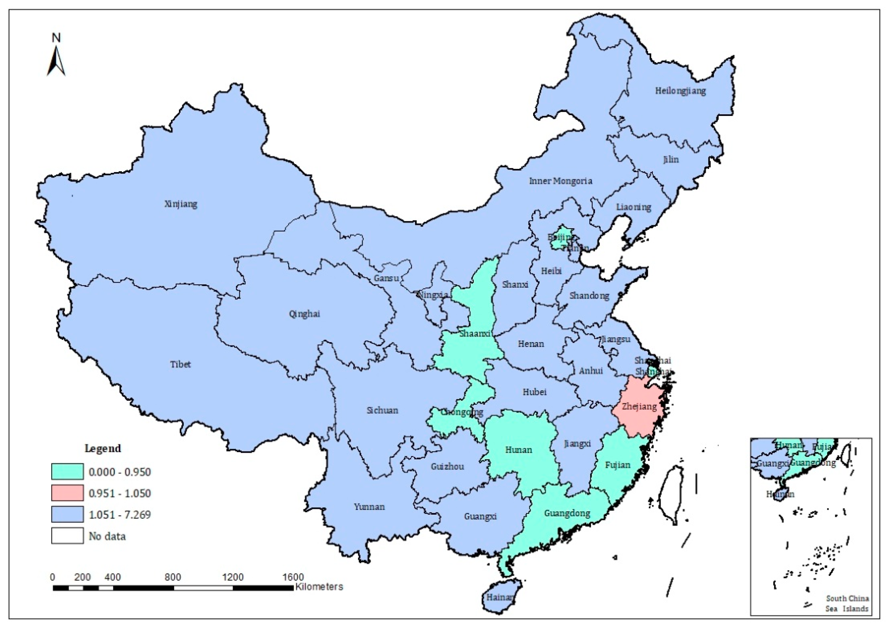
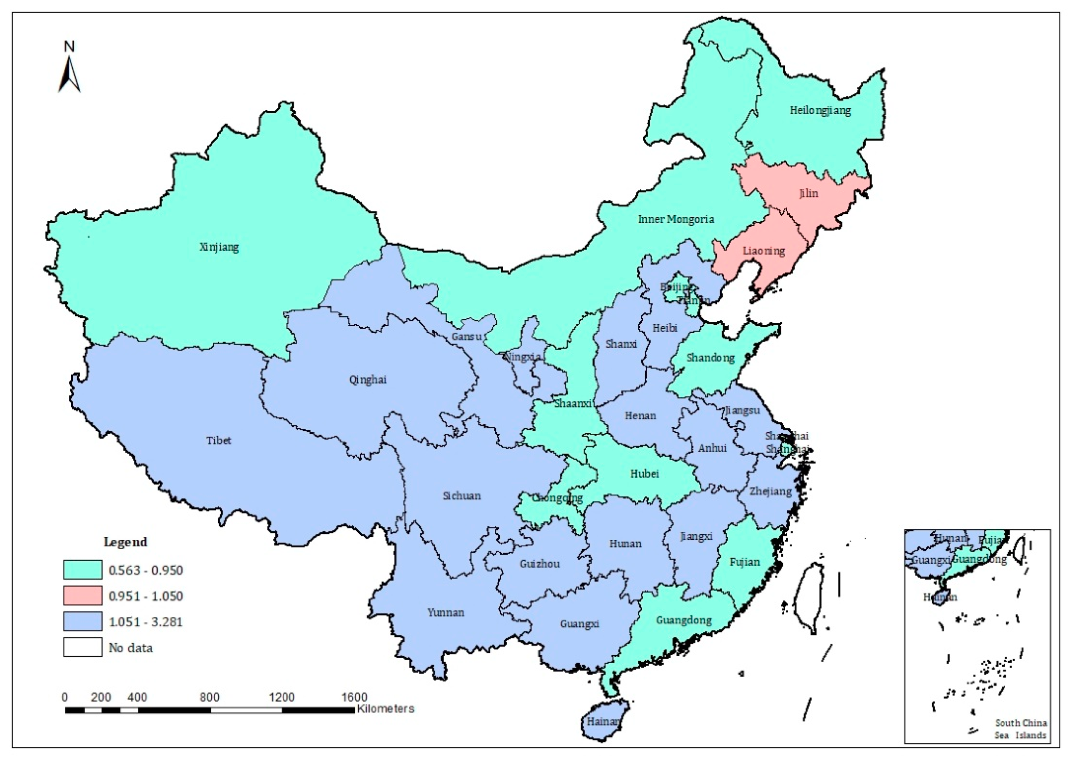
Appendix B. Spatial Distribution of Resource Misallocation in China

Figure A1. Spatial distribution of capital misallocation in China (average from 1997 to 2017).
Sustainability 13 02390 g0a1
Figure A2. Spatial distribution of labor misallocation in China (average from 1997 to 2017).
Sustainability 13 02390 g0a2

Appendix C. Variation Trend of Industrial TFP for Each Province during 1997–2017

Table A1. The variation trends of industrial TFP for 31 provinces.
199719981999200020012002200320042005200620072008200920102011201220132014201520162017
Beijing1.14 1.42 1.67 2.04 2.22 2.28 2.61 2.89 2.89 3.06 3.21 3.23 3.50 4.00 3.80 3.96 4.02 4.17 4.05 4.09 3.93
Tianjin1.14 1.08 1.40 1.62 1.89 2.21 2.47 2.89 3.29 3.59 3.80 4.18 4.81 5.36 6.02 6.58 7.05 7.60 8.70 10.57 10.81
Hebei1.15 1.30 1.55 1.71 1.89 2.08 2.24 2.45 2.67 2.95 3.26 3.51 3.66 3.94 4.27 4.55 4.76 4.85 4.94 5.08 5.16
Shanxi1.10 1.15 1.22 1.26 1.31 1.41 1.47 1.49 1.48 1.49 1.62 1.63 1.53 1.67 1.82 1.97 2.06 2.09 2.02 2.01 2.16
Inner Mongoria1.18 1.51 1.67 1.96 2.38 2.67 2.73 3.03 3.26 3.77 4.19 4.87 5.58 6.04 6.52 6.95 6.91 7.40 8.78 10.23 11.73
Liaoning1.11 1.23 1.39 1.57 1.75 2.03 2.12 2.33 2.53 2.78 3.19 3.65 4.13 4.70 5.36 5.86 5.94 6.31 6.55 6.23 6.58
Jilin1.15 1.66 1.95 2.38 2.82 3.17 3.07 3.27 3.32 3.51 3.77 4.14 4.67 5.49 6.31 6.90 7.11 7.33 7.74 8.45 9.05
Heilongjiang1.07 1.38 1.53 1.84 2.07 2.43 2.94 3.10 3.33 3.51 3.54 3.72 3.96 4.37 4.69 5.00 5.17 4.86 5.09 4.73 4.67
Shanghai1.13 1.29 1.42 1.63 2.28 2.44 2.90 3.51 3.79 4.15 4.45 3.96 4.11 4.70 5.02 5.32 5.80 5.92 6.18 6.34 7.09
Jiangsu1.11 1.23 1.37 1.54 1.72 1.96 2.26 2.62 2.97 3.36 3.81 4.31 4.80 5.38 6.03 6.71 7.40 8.02 8.68 9.26 9.91
Zhejiang1.13 1.29 1.55 1.43 1.53 1.69 1.78 1.94 2.10 2.34 2.53 2.71 2.74 2.88 3.06 3.21 3.46 3.65 3.81 4.01 4.33
Anhui1.13 1.26 1.38 1.53 1.70 1.86 1.94 2.01 2.13 2.09 2.08 2.09 2.19 2.45 2.77 2.94 3.06 3.15 3.26 3.37 3.54
Fujian1.13 1.28 1.42 1.53 1.62 1.75 1.86 2.02 2.04 2.15 2.30 2.41 2.53 2.72 3.07 3.40 3.69 3.98 4.17 4.34 4.57
Jiangxi1.19 1.33 1.38 1.42 1.49 1.54 1.52 1.44 1.35 1.25 1.17 1.10 1.04 1.05 1.18 1.26 1.33 1.42 1.48 1.55 1.65
Shandong1.13 1.33 1.43 1.62 1.77 2.00 2.40 2.49 2.76 3.10 3.45 4.07 4.53 4.93 5.36 5.75 6.22 6.62 6.81 7.07 7.48
Henan1.09 1.18 1.30 1.45 1.58 1.73 1.92 2.09 2.19 2.30 2.43 2.66 2.72 2.93 3.17 3.32 3.39 3.55 3.60 3.70 3.85
Hubei1.14 1.51 1.70 2.03 2.31 2.51 2.51 2.80 3.15 3.53 3.87 4.26 4.78 5.81 6.94 7.89 8.80 9.70 10.55 11.40 12.24
Hunan1.14 1.30 1.44 1.57 1.68 1.74 1.75 1.76 1.68 1.68 1.69 1.69 1.67 1.76 1.81 1.95 2.06 2.15 2.26 2.35 2.54
Guangdong1.16 1.33 1.50 1.71 1.89 2.04 2.27 2.57 2.70 3.01 3.42 3.70 3.81 4.12 4.33 4.44 4.54 4.64 4.67 4.70 4.75
Guangxi1.08 1.21 1.28 1.36 1.47 1.67 1.78 1.89 1.88 1.82 1.71 1.70 1.54 1.56 1.55 1.67 1.78 1.72 1.82 1.91 2.02
Hainan1.04 1.44 1.64 1.86 2.06 2.37 2.74 2.99 3.19 3.72 4.61 4.37 4.61 4.95 4.84 4.37 3.94 4.07 4.17 4.21 4.34
Chongqing1.08 1.12 1.25 1.39 1.56 1.72 1.94 2.04 1.97 1.92 1.96 2.03 2.10 2.29 2.35 2.40 2.44 2.50 2.53 2.61 2.79
Sichuan1.10 1.20 1.28 1.37 1.47 1.58 1.73 1.94 2.18 2.42 2.62 2.86 3.06 3.57 4.19 4.60 4.95 5.18 5.42 5.68 6.00
Guizhou1.10 1.22 1.36 1.41 1.42 1.51 1.80 1.91 1.84 1.76 1.77 1.69 1.63 1.67 1.73 1.76 1.75 1.75 1.77 1.74 1.76
Yunnan1.13 1.28 1.56 1.69 1.80 1.99 2.17 2.00 1.85 1.86 1.87 1.81 1.74 1.74 1.81 1.84 1.84 1.92 2.04 2.10 2.29
Tibet0.96 0.94 0.94 0.90 0.90 0.90 0.64 0.55 0.43 0.37 0.38 0.35 0.35 0.28 0.29 0.20 0.20 0.20 0.15 0.09 0.07
Shaanxi1.12 1.25 1.36 1.45 1.56 1.72 1.77 1.99 2.01 1.95 1.89 1.86 1.66 1.64 1.66 2.13 2.22 2.27 2.29 2.34 2.46
Gansu1.10 1.32 1.40 1.64 1.84 2.00 2.05 2.20 2.40 2.59 2.83 2.88 2.99 3.27 3.61 3.94 4.23 4.60 4.98 5.33 5.31
Qinghai1.18 1.32 1.49 2.16 2.50 2.33 2.81 3.16 3.67 3.95 4.40 5.23 5.63 6.15 10.50 11.36 10.93 12.11 13.15 17.04 14.04
Ningxia1.10 1.30 1.38 1.57 1.68 1.83 1.85 1.89 2.06 2.15 2.32 2.60 2.63 3.01 4.16 4.62 4.76 4.32 4.74 5.23 5.42
Xinjiang1.13 1.17 1.33 1.71 2.00 2.14 2.03 2.19 1.98 2.32 2.48 2.81 2.96 3.10 3.05 3.32 3.26 3.60 4.04 4.36 4.33

Appendix D. Robustness Test Results

Table A2. The impacts of environmental regulation and resource misallocation on industrial TFP using inverse distance matrix instead of queen adjacency matrix.
VariableTFP
(1)(2)(3)(4)
ER−1.234 ** (0.483)−1.286 *** (0.486)
ER20.337 (0.264)0.347 (0.266)
MisK −0.718 *** (0.114)−0.671 *** (0.105)
MisL −0.403 ** (0.180)−0.189 ** (0.081)
Lnpgdp1.680 *** (0.425)2.130 *** (0.514)1.019 ** (0.518)1.174 ** (0.488)
Indstrc−10.452 *** (1.915)−8.907 *** (2.371)−5.242 ** (2.306)−4.199 * (2.084)
Lnfdi−0.86 3*** (0.076)−0.853 *** (0.079)−0.678 *** (0.079)−0.582 *** (0.071)
Lnexpdt0.962 *** (0.299)1.008 ** (0.482)0.378 (0.473)0.364 (0.426)
W × ER −6.689 *** (2.433)
W × ER2 3.483 *** (0.982)
W × MisK −3.277 *** (1.088)
W × MisL 4.399 ** (2.067)
W × Lnpgdp −5.025 *** (1.339) −5.541 * (3.256)
W × Indstrc −13.606 ** (5.476) −82.951 *** (12.643)
W × Lnfdi 0.745 ** (0.361) 3.938 *** (0.745)
W × Lnexpdt 3.005 *** (0.980) 0.044(3.477)
Spatial ρ 0.118 ** (0.051) 0.239 * (0.157)
R20.7690.7830.7950.842
N. Observation 651651651651
fixed effects of provinces YesYesYesYes
fixed effects of years NoNoYesYes
Robust LM-lag 1.907 [0.167] 32.604 *** [0.000]
Robust LM-error 3.957 ** [0.047] 45.565 *** [0.000]
LR spatial FE 565.545 *** [0.000] 549.485 *** [0.000]
LR year FE 10.828 [0.966] 35.878 ** [0.023]
Wald spatial lag 33.068 *** [0.000] 168.791 *** [0.000]
Wald spatial error 31.044 *** [0.000] 163.145 *** [0.000]
Hausman test 98.976 *** [0.000] 150.216 *** [0.000]
Note: The value of standard errors is in the parenthesis, and that of p-values in the square bracket. ***, **, and * represent the significance level of 1%, 5%, and 10%, respectively. The same is as below.
Table A3. Spatial effects of environmental regulation and resource misallocation on industrial TFP using inverse distance matrix instead of queen adjacency matrix.
Direct EffectSpatial Spillover EffectTotal Effect
(1)ER --> TFP−1.286 ** (0.497)−6.850 *** (2.475)−8.136 *** (2.512)
(2)ER2 --> TFP0.349 (0.262)3.546 *** (0.980)3.895 *** (1.001)
(3)MisK --> TFP−0.704 *** (0.108)−2.829 *** (0.981)−3.533 *** (0.984)
(4)MisL --> TFP−0.191 ** (0.076)3.609 ** (1.865)3.418 *** (1.910)
(5)ER --> MisK−0.508 *** (0.099)−0.080 (0.343)−0.588 * (0.350)
(6)ER --> MisL−0.096 (0.062)−0.251 ** (0.119)−0.347 * (0.197)
Table A4. The impacts of environmental regulation on resource misallocation using inverse distance matrix instead of queen adjacency matrix.
VariableMisK MisL
(1)(2)(3)(4)
ER−0.597 *** (0.097)−0.458 *** (0.094)−0.087 (0.061)−0.105 *(0.059)
Lnpgdp−0.115 *** (0.019)−0.853 *** (0.191)−1.181 *** (0.119)−1.177 *** (0.119)
Indstrc5.359 *** (0.890)5.349 *** (0.870)2.688 *** (0.561)2.461 *** (0.545)
Lnfdi0.171 *** (0.030)0.147 ***(0.030)0.084 *** (0.019)0.081 *** (0.019)
Lnexpdt−1.308 *** (0.181)−1.232 *** (0.176)−0.496 *** (0.114)−0.498 *** (0.110)
W × ER −0.088 (0.470) −0.397 ** (0.196)
W × Lnpgdp 1.223 (1.295) 1.534 * (0.839)
W × Indstrc −5.147 (4.959) −1.387 (3.114)
W × Lnfdi 0.486 *** (0.033) 0.152 *** (0.024)
W × Lnexpdt −2.996 ** (1.471) −2.190 ** (0.910)
Spatial ρ 0.512 *** (0.174) 0.640 *** (0.178)
R20.8990.9050.8350.846
N. Observation651651651651
fixed effects of provincesYesYesYesYes
fixed effects of yearsYesYesYesYes
Robust LM-lag8.654 *** [0.003] 5.148 ** [0.023]
Robust LM-error10.351 *** [0.001] 8.262 *** [0.004]
LR spatial FE1153.430 *** [0.000] 948.556 *** [0.000]
LR year FE81.025 *** [0.000] 160.132 *** [0.000]
Wald spatial lag 16.134 *** [0.000] 16.852 *** [0.000]
Wald spatial error 16.251 *** [0.000] 19.275 *** [0.000]
Hausman test 28.204*** [0.003] 32.363 *** [0.000]
Table A5. The resource reallocation effects of environmental regulation on industrial TFP using inverse distance matrix instead of queen adjacency matrix.
VariableTFP
(1)(2)(3)
ER−0.811 *** (0.212)−0.749 *** (0.220)−0.783 *** (0.213)
MisK−0.733 *** (0.093) −0.675 *** (0.104)
MisL −0.494 *** (0.159)−0.431 *** (0.168)
Lnpgdp1.077 ** (0.437)1.066 ** (0.490)1.225 ** (0.486)
Indstrc−3.799 * (2.063)−7.351 *** (2.089)−4.032 * (2.064)
Lnfdi−0.569 *** (0.070)−0.642 *** (0.072)−0.576 *** (0.070)
Lnexpdt0.599 (0.417)0.658 (0.418)0.443 (0.423)
W × ER0.618 (1.068)1.063 (1.119)0.931 (1.083)
W × MisK4.716 *** (0.867) 3.351 *** (1.079)
W × MisL 10.206 *** (1.726)4.140 * (2.081)
W × Lnpgdp−8.764 *** (2.974)−5.232 ** (2.359)−6.426 * (3.264)
W × Indstrc−85.306 *** (12.372)−68.761 *** (12.087)−80.904 *** (12.512)
W × Lnfdi3.630 *** (0.737)4.286 *** (0.766)3.835 *** (0.742)
W × Lnexpdt0.564 (3.456)1.395 (3.422)0.402 (3.461)
Spatial ρ 0.208 *** (0.057)0.385 *** (0.161)0.202 *** (0.054)
R20.8440.8340.845
N. Observation651651651
fixed effects of provincesYesYesYes
fixed effects of yearsYesYesYes
Wald spatial lag173.920 *** [0.000]161.405 *** [0.000]172.680 *** [0.000]
Wald spatial error165.728 *** [0.000]159.462 *** [0.000]165.269 *** [0.000]
Hausman test128.040 *** [0.000]109.473 *** [0.000]128.343 *** [0.000]

References

  1. Liu, H.W.; Zheng, S.L.; Zuo, W.T. The Influence Mechanism of Environmental Regulation on TFP of Enterprises. Sci. Res. Manag. 2016, 37, 33–41. [Google Scholar]
  2. Boyed, G.A.; McClelland, J.D. The Impact of Environmental Constraints on Productivity Improvement in Integrated Paper Plants. J. Environ. Econ. Manag. 1999, 38, 121–142. [Google Scholar] [CrossRef]
  3. Tanguay, G.A.; Rajaonson, J.; Lefebvre, J.-F.; Lanoie, P. Measuring the Sustainability of Cities: An Analysis of the Use of Local Indicators. Ecol. Indic. 2010, 10, 407–418. [Google Scholar] [CrossRef]
  4. Greenstone, M.; List, J.A.; Syverson, C. The Effects of Environmental Regulation on the Competitiveness of U.S. Manufacturing; NBER Working Paper No. 18392; 2012; Available online: https://www.nber.org/papers/w18392.2012 (accessed on 12 November 2020).
  5. Zhu, Y.; Wang, Z.; Qiu, S.; Zhu, L. Effects of Environmental Regulations on Technological Innovation Efficiency in China’s Industrial Enterprises: A Spatial Analysis. Sustainability 2019, 11, 2186. [Google Scholar] [CrossRef] [Green Version]
  6. Hou, B.Q.; Wang, B.; Du, M.Z.; Zhang, N. Does the SO2 Emissions Trading Scheme Encourage Green Total Factor Productivity? An Empirical Assessment on China’s Cities. Environ. Sci. Pollut. Res. 2020, 27, 6375–6388. [Google Scholar] [CrossRef] [PubMed]
  7. Porter, M.E.; Van der Linde, C. Toward a New Conception of the Environment-Competitiveness Relationship. J. Econ. Perspect. 1995, 9, 97–118. [Google Scholar] [CrossRef]
  8. Hamamoto, M. Environmental Regulation and the Productivity of Japanese Manufacturing Industries. Resour. Energy Econ. 2006, 28, 299–312. [Google Scholar] [CrossRef]
  9. Ambec, S.; Cohen, M.A.; Elgie, S.; Lanoie, P. The Porter Hypothesis at 20: Can Environmental Regulation Enhance Innovation and Competitiveness. Rev. Environ. Econ. Policy. 2013, 7, 2–22. [Google Scholar] [CrossRef] [Green Version]
  10. Jorge, M.L.; Madueño, J.H.; Martínez-Martínez, D.; Sancho, M.P.L. Competitiveness and Environmental Performance in Spanish Small and Medium Enterprises: Is there a Direct Link? J. Clean. Prod. 2015, 101, 26–37. [Google Scholar] [CrossRef]
  11. Sun, X.M.; Wang, J. Environmental Regulation, Induced R&D and Firms’ TFP—Porter Hypothesis Reexamined. J. Xi’an Jiaotong Univ. (Soc. Sci.) 2016, 36, 10–16. [Google Scholar]
  12. Shen, Y.C.; Yue, S.J.; Sun, S.Q.; Guo, M.Q. Sustainable Total Factor Productivity Growth: The Case of China. J. Clean. Prod. 2020, 256, 120727. [Google Scholar] [CrossRef]
  13. Lou, Y.; Tian, Y.; Tang, X. Does Environmental Regulation Improve and Enterprise’s Productivity?—Evidence from China’s Carbon Reduction Policy. Sustainability 2020, 12, 6742. [Google Scholar] [CrossRef]
  14. Zhao, M.L.; Liu, F.Y.; Sun, W.; Tao, X. The Relationship between Environmental Regulation and Green Total Factor Productivity in China: An Empirical Study Based on the Panel Data of 177 Cities. Int. J. Environ. Res. Public Health 2020, 17, 5287. [Google Scholar] [CrossRef] [PubMed]
  15. Johnstone, N.; Managi, S.; Rodriguez, M.C.; Hascic, I.; Fujii, H.; Souchier, M. Environmental Policy Design, Innovation and Efficiency Gains in Electricity Generation. Energy Econ. 2017, 63, 106–115. [Google Scholar] [CrossRef]
  16. He, Y.M.; Luo, Q. Environmental Regulation, Technological Innovation and Industrial Total Factor Productivity of China—Reexamination of the Strong Potter Hypothesis. Soft Sci. 2018, 32, 20–25. [Google Scholar]
  17. Li, B.; Peng, X.; Ouyang, M.K. Environmental Regulation, Green Total Factor Productivity and the Transformation of China’s Industrial Development Mode—Analysis Based on Data of China’s 36 Industries. China Ind. Econ. 2013, 4, 56–68. [Google Scholar]
  18. Elgin, C.; Oztunali, O. Environmental Kuznets Curve for the Informal Sector of Turkey (1950–2009). Panoeconomicus 2014, 61, 471–485. [Google Scholar] [CrossRef] [Green Version]
  19. Albrizio, S.; Kozluk, T.; Zipperer, V. Environmental Policies and Productivity Growth: Evidence across Industries and Firms. J. Environ. Econ. Manag. 2017, 81, 209–226. [Google Scholar] [CrossRef]
  20. Zhao, X.M.; Liu, C.J.; Yang, M. The Effects of Environmental Regulation on China’s Total Factor Productivity: An Empirical Study of Carbon-Intensive Industries. J. Clean. Prod. 2018, 179, 325–334. [Google Scholar] [CrossRef]
  21. Wang, J.; Liu, B. Environmental Regulation and Enterprises’ TFP—An Empirical Analysis Based on China’s Industrial Enterprises Data. China Ind. Econ. 2014, 3, 44–56. [Google Scholar]
  22. Jin, Y.G.; Chang, R. Environmental Regulation and Industrial Total Factor Productivity: An Empirical Study on the Dynamic Panel Data of 280 Prefecture Level Cities. J. Econ. Prob. 2016, 11, 18–23. [Google Scholar]
  23. Tong, J.; Liu, W.; Xue, J. Environmental Regulation, Factor Input Structure and Industrial Transformation. Econ. Res. J. 2016, 51, 43–57. [Google Scholar]
  24. Barbera, A.J.; McConnell, V.D. The Impact of Environmental Regulations on Industry Productivity: Direct and Indirect Effects. J. Environ. Econ. Manag. 1990, 18, 50–65. [Google Scholar] [CrossRef]
  25. Zhao, X.M.; Liu, C.J.; Sun, C.W.; Yang, M. Does Stringent Environmental Regulation Lead to a Carbon Haven Effect? Evidence from Carbon-intensive Industries in China. Energy Econ. 2020, 86, 104631. [Google Scholar] [CrossRef]
  26. Chen, C.F.; Han, J.; Mao, Y.L. Environmental Regulation, Industrial Heterogeneity and Industrial Green Growth in China—a Nonlinear Test from the Perspective of Total Factor Productivity. J. Shanxi Univ. Financ. Econ. 2018, 40, 65–80. [Google Scholar]
  27. Ju, K.Y.; Zhou, D.J.; Wu, J.M. Can Environmental Regulation a “Win-Win” Strategy?—Strong Porter Hypothesis Research on China’s Industry. J. Beijing Inst. Technol. (Soc. Sci. Ed.) 2020, 22, 21–28. [Google Scholar]
  28. Lee, E. Environmental Regulation and Financial Performance in China: An Integrated View of the Porter Hypothesis and Institutional Theory. Sustainability 2020, 12, 10183. [Google Scholar] [CrossRef]
  29. Berman, E.; Bui, L.T.M. Environmental Regulation and Productivity: Evidence from Oil Refineries. Rev. Econ. Stat. 2001, 83, 498–510. [Google Scholar] [CrossRef] [Green Version]
  30. Piot-Lepetit, I.; Le Moing, M. Productivity and Environmental Regulation: The Effect of the Nitrates Directive in the French Pig Sector. Environ. Resour. Econ. 2007, 38, 433–446. [Google Scholar] [CrossRef]
  31. Lanoie, P.; Patry, M.; Lajeunesse, R. Environmental Regulation and Productivity: Testing the Porter Hypothesis. J. Prod. Anal. 2008, 30, 121–128. [Google Scholar] [CrossRef]
  32. Hancevic, P.I. Environmental Regulation and Productivity: The Case of Electricity Generation under the CAAA-1990. Energy Econ. 2016, 60, 131–143. [Google Scholar] [CrossRef]
  33. Manello, A. Productivity Growth, Environmental Regulation and Win-win Opportunities: The Case of Chemical Industry in Italy and Germany. Eur. J. Oper. Res. 2017, 262, 733–743. [Google Scholar] [CrossRef]
  34. Guner, N.; Ventura, G.; Xu, Y. Macroeconomic Implications of Size-Dependent Policies. Rev. Econ. Dyn. 2008, 11, 721–744. [Google Scholar] [CrossRef] [Green Version]
  35. Song, S.; Yi, D.T. The Fundraising Efficiency in U.S. Non-Profit Art Organizations: An Application of a Bayesian Estimation Approach using the Stochastic Frontier Production Model. J. Prod. Anal. 2011, 35, 171–180. [Google Scholar] [CrossRef]
  36. Buera, F.J.; Shin, Y. Financial Frictions and the Persistence of History: A Quantitative Exploration. J. Political Econ. 2013, 121, 221–272. [Google Scholar] [CrossRef] [Green Version]
  37. Fontagne, L.; Santoni, G. Agglomeration Economies and Firm-Level Labor Misallocation. J. Econ. Geogr. 2019, 19, 251–272. [Google Scholar] [CrossRef]
  38. Buera, F.J.; Kaboski, J.P.; Shin, Y. Finance and Development: A Tale of Two Sectors. Am. Econ. Rev. 2011, 101, 1964–2002. [Google Scholar] [CrossRef] [Green Version]
  39. Jovanovic, B. Misallocation and Growth. Am. Econ. Rev. 2014, 104, 1149–1171. [Google Scholar] [CrossRef] [Green Version]
  40. Qian, X.; Cai, Y. A Survey on Measurements of Resource Misallocation. J. Beijing Technol. Bus. Univ. (Soc. Sci.) 2014, 29, 116–126. [Google Scholar]
  41. Hsieh, C.T.; Klenow, P.J. Misallocation and Manufacturing TFP in China and India. Quart. J. Econ. 2009, 124, 1403–1448. [Google Scholar] [CrossRef] [Green Version]
  42. Aoki, S. A Simple Accounting Framework for the Effect of Resource Misallocation on Aggregate Productivity. J. Jpn. Int. Econ. 2012, 26, 473–494. [Google Scholar] [CrossRef] [Green Version]
  43. Bartelsman, E.; Haltiwanger, J.; Scarpetta, S. Cross-Country Differences in Productivity: The Role of Allocation and Selection. Am. Econ. Rev. 2013, 103, 305–334. [Google Scholar] [CrossRef] [Green Version]
  44. Midrigan, V.; Xu, D.Y. Finance and Misallocation: Evidence from Plant-Level Data. Am. Econ. Rev. 2014, 104, 422–458. [Google Scholar] [CrossRef] [Green Version]
  45. Tombe, T.; Winter, J. Environmental Policy and Misallocation: The Productivity Effect of Intensity Standards. J. Environ. Econ. Manag. 2015, 72, 137–163. [Google Scholar] [CrossRef]
  46. Han, C.; Zhang, W.G.; Feng, Z.B. How Does Environmental Regulation Remove Resource Misallocation—An Analysis of the First Obligatory Pollution Control in China. China Ind. Econ. 2017, 4, 115–134. [Google Scholar]
  47. Dong, Z.Q.; Hu, S.M.; Wang, L.H. Misallocation of Innovation Factors: A Comparative Study Based on the Spatial Spillover Effects. Zhejiang Acad. J. 2020, 2, 136–145. [Google Scholar]
  48. Li, G.; Dong, M.J.; Shen, K.T. The Impact of Intensified Environmental Regulations Policies on China’s Economic Growth—An Assessment Based on CGE Model. China Ind. Econ. 2012, 11, 5–17. [Google Scholar] [CrossRef]
  49. Li, L.; Tao, F. Selection of Optimal Environmental Regulation Intensity for Chinese Manufacturing Industry—Based on the Green TFP Perspective. China Ind. Econ. 2012, 5, 70–82. [Google Scholar]
  50. Anselin, L.; Bera, A.K.; Florax, R.; Yoon, M.J. Simple Diagnostic Tests for Spatial Dependence. Reg. Sci. Urban. Econ. 1996, 26, 77–104. [Google Scholar] [CrossRef]
  51. LeSage, J.P.; Pace, R.K. Introduction to Spatial Econometrics; Taylor and Francis: Boca Raton, FL, USA, 2009. [Google Scholar]
  52. Wang, Y.; Li, J.M. Measurement of Environmental Regulation Intensity, Potential Problems and its Correction. Collect. Essays Financ. Econ. 2015, 194, 98–106. [Google Scholar]
  53. Jin, L.Q. Analysis of Resources Misallocation among Regions from 1992 to 2015. Soc. Sci. Beijing 2018, 1, 57–66. [Google Scholar]
  54. Zhang, J.Q.; Gong, E.Z.; Sun, Y.Y. How Will Environmental Regulation Effect TFP of Manufacturing in Yangtze River Economic Belt? Stud. Sci. Sci. 2019, 37, 1558–1569. [Google Scholar]
  55. Kumar, S.; Managi, S. Environmental Productivity and Kuznets Curve. Ecol. Econ. 2008, 65, 432–440. [Google Scholar]
  56. Elhorst, J.P. Spatial Econometrics: From Cross-Sectional Data to Spatial Panels; Springer: New York, NY, USA, 2014. [Google Scholar]
  57. Shapiro, J.S.; Walker, R. Why Is Pollution from US Manufacturing Declining? The Roles of Environmental Regulation, Productivity, and Trade. Am. Econ. Rev. 2018, 108, 3814–3854. [Google Scholar] [CrossRef] [Green Version]
  58. Restuccia, D.; Rogerson, R. Policy Distortions and Aggregate Productivity with Heterogeneous Establishments. Rev. Econ. Dyn. 2008, 11, 707–720. [Google Scholar] [CrossRef]
  59. Kim, H.; Kim, D.; Paul, C.; Lee, C.K. The Spatial Allocation of Hospitals With Negative Pressure Isolation Rooms in Korea: Are We Prepared for New Outbreaks? Int. J. Health Policy Manag. 2020, 9, 475–483. [Google Scholar]
  60. Brandt, L.; Tombe, T.; Zhu, X. Factor Market Distortions across Time, Space and Sectors in China. Rev. Econ. Dyn. 2013, 16, 39–58. [Google Scholar] [CrossRef] [Green Version]
Table 1. Descriptive statistics of variables.
VariableDescriptionMeanStd.DevMinMax
TFPIndustrial total factor productivity3.0282.1790.06617.041
EREnvironmental regulation intensity0.2810.2410.0232.548
MisKDegree of capital misallocation1.5001.2360.2349.840
MisLDegree of labor misallocation1.1540.6100.3414.042
LnpgdpThe level of economic development9.8280.9137.71911.768
IndstrcIndustrial structure0.8650.0740.6220.996
LnfdiDegree of openness11.7922.0000.69315.090
LnexpdtGovernment regulation and control ability6.9411.2703.5159.618
Table 2. The impacts of environmental regulation and resource misallocation on industrial total factor productivity (TFP).
VariableTFP
(1)(2)(3)(4)
ER−1.234 ** (0.483)−1.184 ** (0.485)
ER20.337 (0.264)0.277 (0.264)
MisK −0.718 *** (0.114)−0.726 *** (0.117)
MisL −0.403 ** (0.180)−0.368 ** (0.175)
Lnpgdp1.680 *** (0.425)2.972 *** (0.557)1.019 ** (0.518)1.200 ** (0.544)
Indstrc−10.452 *** (1.915)−11.808 *** (2.329)−5.242 ** (2.306)−6.430 *** (2.287)
Lnfdi−0.863 *** (0.076)−0.832 *** (0.079)−0.678 *** (0.079)−0.662 *** (0.074)
Lnexpdt0.962 *** (0.299)0.660 (0.502)0.378 (0.473)0.254 (0.473)
W×ER −1.760 * (0.970)
W×ER2 1.335 *** (0.515)
W×MisK −1.142 *** (0.240)
W×MisL 0.011 * (0.006)
W×Lnpgdp −3.929 *** (0.742) −2.857 *** (0.918)
W×Indstrc −7.950 ** (3.287) −14.848 *** (4.377)
W×Lnfdi 0.367 ** (0.156) 0.903 *** (0.163)
W×Lnexpdt 2.118 *** (0.635) 0.166(0.909)
Spatial ρ 0.098 * (0.054) 0.187 *** (0.053)
R20.7690.7910.7950.826
N. Observation651651651651
fixed effects of provincesYesYesYesYes
fixed effects of years NoNoYesYes
Robust LM-lag 1.907 [0.167] 32.604 *** [0.000]
Robust LM-error 3.957 ** [0.047] 45.565 *** [0.000]
LR spatial FE 565.545 *** [0.000] 549.485 *** [0.000]
LR year FE 10.828 [0.966] 35.878 ** [0.023]
Wald spatial lag 60.682 *** [0.000] 99.919 *** [0.000]
Wald spatial error 55.955 *** [0.000] 78.281 *** [0.000]
Hausman test 32.119 *** [0.002] 80.843 *** [0.000]
Note: The value of standard errors is in the parenthesis, and that of p-values in the square bracket. ***, **, and * represent the significance level of 1%, 5%, and 10%, respectively. The same is as below.
Table 3. Spatial effects of environmental regulation and resource misallocation on industrial TFP.
Direct EffectSpatial Spillover EffectTotal Effect
(1)ER --> TFP−1.221 ** (0.477)−2.040 * (1.064)−3.261 *** (1.114)
(2)ER2 --> TFP0.304 (0.271)1.474 *** (0.571)1.778 *** (0.641)
(3)MisK --> TFP−0.678 *** (0.124)−1.195 *** (0.284)−1.873 *** (0.312)
(4)MisL --> TFP−0.372 ** (0.176)0.015 ** (0.007)−0.357 *** (0.097)
(5)ER --> MisK−0.381 *** (0.096)−0.092 (0.202)−0.473 ** (0.223)
(6)ER --> MisL−0.083 (0.061)−0.243 ** (0.121)−0.325 ** (0.133)
Table 4. The impacts of environmental regulation on resource misallocation.
VariableMisK MisL
(1)(2)(3)(4)
ER−0.597 *** (0.097)−0.338 *** (0.093)−0.087 (0.061)−0.083 (0.060)
Lnpgdp−0.115 *** (0.019)−0.788 *** (0.208)−1.181 *** (0.119)−1.212 *** (0.133)
Indstrc5.359 *** (0.890)6.519 *** (0.893)2.688 *** (0.561)2.503 *** (0.577)
Lnfdi0.171 *** (0.030)0.144 *** (0.030)0.084 *** (0.019)0.087 *** (0.019)
Lnexpdt−1.308 *** (0.181)−0.822 *** (0.188)−0.496 *** (0.114)−0438 *** (0.121)
W × ER −0.097(0.189) −0.253 ** (0.122)
W × Lnpgdp 2.176 *** (0.331) 2.090 * (1.132)
W × Indstrc −1.151 (1.757) −0.262 (0.227)
W × Lnfdi 0.185 *** (0.067) 0.136 *** (0.044)
W × Lnexpdt −2.141 *** (0.365) −0.317 (0.231)
Spatial ρ 0.529 *** (0.057) 0.046 ** (0.021)
R20.8990.9070.8350.841
N. Observation651651651651
fixed effects of provincesYesYesYesYes
fixed effects of yearsYesYesYesYes
Robust LM-lag8.654 *** [0.003] 5.148 ** [0.023]
Robust LM-error10.351 *** [0.001] 8.262 *** [0.004]
LR spatial FE1153.430 *** [0.000] 948.556 *** [0.000]
LR year FE81.025 *** [ 0.000] 160.132 *** [0.000]
Wald spatial lag 50.950 *** [0.000] 16.761 *** [0.005]
Wald spatial error 50.965 *** [0.000] 16.401 *** [0.006]
Hausman test 81.895 *** [0.000] 31.947 *** [0.002]
Table 5. The resource reallocation effects of environmental regulation on industrial TFP.
VariableTFP
(1)(2)(3)
ER−0.849 *** (0.222)−0.820 *** (0.234)−0.803 *** (0.225)
MisK−0.852 *** (0.095) −0.729 *** (0.111)
MisL −1.028 *** (0.150)−0.358 ** (0.173)
Lnpgdp1.598 *** (0.510)2.010 *** (0.492)1.947 *** (0.479)
Indstrc−6.250 *** (2.262)−9.7605 *** (2.183)−5.776 *** (2.173)
Lnfdi−0.671 *** (0.073)−0.680 *** (0.075)−0.631 *** (0.073)
Lnexpdt0.442 (0.466)0.180 (0.352)−0.103 (0.353)
W × ER0.581 (0.455)0.746 (0.486)0.660 (0.468)
W × MisK1.225 *** (0.207) 0.936 *** (0.229)
W × MisL 1.629 *** (0.339)1.385 *** (0.381)
W × Lnpgdp−2.597 *** (0.823)−2.189 *** (0.860)−2.155 *** (0.837)
W × Indstrc−16.768 *** (4.311)−8.839 ** (4.287)−13.192 *** (4.225)
W × Lnfdi0.855 *** (0.162)0.839 *** (0.160)0.891 *** (0.155)
W × Lnexpdt0.125 (0.900)−0.028 (0.736)0.101 (0.761)
Spatial ρ 0.196 *** (0.052)0.121 ** (0.053)0.174 ***(0.051)
R20.8290.6960.719
N. Observation651651651
fixed effects of provincesYesNoNo
fixed effects of yearsYesYesYes
Wald spatial lag105.767 *** [0.000]98.668 *** [0.000]96.965 *** [0.000]
Wald spatial error81.402 *** [0.000]85.108 *** [0.000]76.138 *** [0.000]
Hausman test20.138 * [0.092]7.287 [0.887]19.705 [0.184]
Publisher’s Note: MDPI stays neutral with regard to jurisdictional claims in published maps and institutional affiliations.

