Article

Impact of Structural Oil Price Shock Factors on the Gasoline Market and Macroeconomy in South Korea

Department of Economics, Dankook University, Yongin-si, Gyeonggi-do 16890, Korea
*
Author to whom correspondence should be addressed.
Sustainability 2021, 13(4), 2209; https://doi.org/10.3390/su13042209
Submission received: 28 January 2021 / Revised: 11 February 2021 / Accepted: 14 February 2021 / Published: 18 February 2021
(This article belongs to the Special Issue Towards Sustainability: Energy and Carbon Efficiency)

Abstract

:
This study decomposed shocks of the global crude oil (GCO) market and Korean gasoline (KG) market into six types using the structural vector auto-regressive model. Breaking down the shocks into six, we analyzed how each shock affects the macroeconomy and gasoline market in Korea. Results of the analysis revealed that the oil supply shock did not cause a large fluctuation in gasoline prices, but it harmed the macroeconomy. By contrast, the two shocks on the demand side of the GCO market caused a large increase in domestic gasoline prices, but they did not negatively affect the macroeconomy. Meanwhile, in the KG market, gasoline-refining shock and gasoline demand shock caused a significant increase in gasoline prices. Both shocks had some negative effects on the Korean macroeconomy at a certain point, but the effects are not as strong as the oil supply shock. However, the gasoline distribution shock in Korea rarely caused negative consequences for major macroeconomic variables. Moreover, analyzing the KG prices through historical decomposition, we found that the two demand-side factors of the GCO market and the demand shock of the KG market have had the most important influence on the gasoline price since the 2000s. From the analysis, the increase in gasoline prices in Korea since the 2000s can be inferred to have no significant negative impact on the macroeconomy. Therefore, the essential factors of price fluctuations must be focused on in analyzing domestic gasoline price and their impact on the macroeconomy.

1. Introduction

Since the 1970s, when South Korea shifted to an industrial structure centered on the heavy and chemical industry and manufacturing, crude oil and extracted gasoline have become an important element that forms the basis of the Korean economy. Particularly, fluctuations in both global oil and domestic gasoline prices and securing stable crude oil are inevitably sensitive to the economy in countries that do not produce crude oil and depend entirely on imports, such as Korea. A series of shocks, such as the collapse of oil prices due to the coronavirus outbreak and high oil prices that appeared in the early 2010s, spread to the domestic gasoline market by importing, refining, and distributing crude oil. This effect is also transmitted to the domestic macroeconomy in a chain. Therefore, implementing related policies without a rigorous study on the underlying cause of the oil price shock can have serious adverse effects on the domestic economy. Moreover, analysis of this and the oil price shock effect that dynamically ripples to the domestic gasoline market and the macroeconomy is necessary.
Despite the importance of oil price shock, studies that comprehensively analyze the series of processes from the global crude oil (GCO) market to the domestic gasoline market and the macroeconomy are relatively insufficient. Particularly, many studies have examined respectively the effects of energy price shocks on the macroeconomy for various countries (Van de Ven and Fouquet (2016), Zerrin and Yasemin (2017), Dramani and Frimpong (2020), Almutairi (2020)), and the relationship between GCO prices and domestic gasoline prices (Borenstein et al. (1997), Manning (1991), Kaufmann and Laskowski (2005), Radchenko and Shapiro (2011), Kuper (2012), Polemis and Fotis (2014), Hong and Lee (2020)) [1,2,3,4,5,6,7,8,9,10,11]. However, studies examining these effects by breaking down the shocks in the GCO and domestic gasoline markets are scarce. Although not as strong as the impact of the GCO market, the shocks inside the domestic gasoline market are also expected to have significant effects on the macroeconomy.
This perception can also be confirmed by Kilian (2010) and Edelstein and Kilian (2009) [12,13]. Kilian (2010) pointed out that a problem exists because previous studies that attempted to link movements of the GCO prices and domestic gasoline prices in each country did not distinguish underlying oil demand and supply factors [12]. Edelstein and Kilian (2009) also pointed out that research on the effect of energy wholesale price shock on the economy is relatively insufficient [13]. Based on this recognition, Kilian (2010) analyzed the ripple effect on the GCO market and the US gasoline market by combining the demand-supply shock of the US gasoline market with the structural vector auto-regressive (SVAR) model of the GCO market used by Kilian (2009) [12,14]. Furthermore, Kang et al. (2019) expanded the analysis by adding a policy uncertainty shock to Kilian (2010)’s model [12,15]. Although these studies revealed that reactions in the GCO market and the US gasoline market may appear differently depending on the impact factors, the absence of the analysis of the effect on the macroeconomy remains a limitation. Various studies have also examined the relationship between the GCO market and the domestic gasoline market in Korea, but these studies are limited because they have not been decomposed into detailed factors. Consequently, the reactions to the domestic gasoline market and the macroeconomy by combining the shocks in the GCO and domestic gasoline market into one frame and decomposing them in detail have not been sufficiently studied.
Based on such awareness of a problem, this study applies and expands the methodology of Kilian (2009) and Kilian (2010) [12,14]. In other words, the impact of structural oil price shock factors on the Korean gasoline (KG) market and the macroeconomy is analyzed using the SVAR model in which the KG market is combined with the GCO market. According to Kilian (2010), the US gasoline market was combined with the GCO market; however, the gasoline market was simply divided into refining shock and gasoline demand shock [12]. The shocks must be further subdivided, and the impact of gasoline distribution must be considered to examine subtle differences in the effects of the fundamental factors in the gasoline market on the overall macroeconomy.
Therefore, this study decomposes the shocks into (1) oil supply shock (changes in crude oil production); (2) global aggregate demand shock (demand changes for overall industrial goods caused by international economic cycles); and (3) oil-specific demand shock (a preliminary demand or speculative demand shock and a shock caused by changes in the uncertainty that cannot be explained by oil supply shock and global aggregate demand shock) in the GCO market. In addition, by combining the shocks of the GCO market with the impacts of the KG market, this article distinguishes (4) KG-refining shock (fluctuations in gasoline refining cost or disturbance in the operation of refining facilities, i.e., a sort of wholesale shock); (5) KG distribution shock (fluctuations in gasoline distribution cost or change in circulation limit, i.e., a sort of retail shock); and (6) KG demand shock (changes in domestic gasoline demand) in the KG market. Using the SVAR model constructed in this way, we examine how the six fundamental impact factors affect the international oil market and the domestic gasoline market, respectively. In addition, the different effects of each shock will be revealed by examining how the six decomposed shocks affect the major variables of the Korean macroeconomy. Moreover, the historical contribution of each shock to the gasoline price in Korea will also be examined.
Based on this, the hypotheses for the study are as follows. First of all, we verify again that the three shocks in the GCO market (oil supply shock, global aggregate demand shock, and oil-specific demand shock) have heterogeneous effects on global crude oil prices and Korean gasoline prices since the late 1990s. In particular, the two demand factors are expected to be relatively more influential than the impact of oil supply on global crude oil prices, and the similar situation is expected to appear in Korean gasoline prices depending on the relationship between international oil prices and domestic gasoline prices (Kilian (2009, 2010), Kang et al. (2019)) [12,14,15]. In addition, oil supply shock is expected to cause stagflation and economic recession in the Korean macroeconomy according to the usual economic logic, but two demand factors are expected to have a positive or at least not so large negative impact relatively on the Korean macroeconomy (Lippi and Nobili (2012), Baumeister and Peersman (2013), Peersman and Van Robays (2009, 2012)) [16,17,18,19].
Meanwhile, among the three shocks in the KG market, the influence of refining shock is expected to be relatively long-term compared to distribution shock. In the case of the KG market, four major private refining companies (SK Innovation, GS Caltex, Hyundai Oil Bank, and S-OIL) occupy the majority of the market, which is an oligopolistic structure (Kim and Lee (2014)) [20]. Therefore, it is expected that it will be difficult for other companies to increase the corresponding reduction in gasoline supply in the event of a breakdown or trouble in the operation of refining facilities from certain companies. In order to maintain the previous gasoline supply, other companies need to invest in additional refining facilities to a corresponding extent. However, not only does it take time to expand refining facilities, but even if the refining facilities are expanded, it could result in a decrease in domestic gasoline prices if the repair is completed by a company that had the problem previously. As a result, it is expected that other companies would not try to expand their refining facilities or increase their gasoline supply recklessly, even if certain companies experience problems with their facilities. Therefore, the effect of raising domestic gasoline prices is relatively long-term. Furthermore, the long-term effect of price hikes from the factor of domestic gasoline supply is expected to cause some economic recession eventually.
On the other hand, in the case of gas stations that suffer from problems caused by KG distribution shock, rising prices due to this shock can cause immediate losses compared to gas stations that do not raise prices around them. This means that the gasoline retail market is relatively competitive in terms of space and gas station characteristics in Korea (Kim and Lee (2014), Kim (2018)) [20,21]. Therefore, it is expected that there will be an inducement for gas stations to quickly re-cut prices in some way. In addition, it seems that this shock could also be partially resolved through inventory sales. As a result, the effect of price increase is expected to be short-term or temporary, and the short-term increase in domestic gasoline prices is not expected to put much pressure on the macroeconomy.
Finally, in the case of KG demand shock, the price increase is expected to be the largest and most continuous among the three shocks in the KG market. If gasoline consumption suddenly increases due to the impact of KG demand shock, gasoline prices are likely to rise strongly because gasoline suppliers cannot expand facility investment in the short term and cannot make facility investment due to uncertainty over whether consumption increases are continuous or temporary. As a result, it is expected that if the price increase effect continues despite the economic stimulus effects by increased demand for gasoline, it could serve as a factor causing some economic recession. Furthermore, consumption increases or maintains despite a steady increase in prices, the budget burden of households or corporates may eventually reduce demand for other goods, and if this effect is greater, it could be a factor in private consumption, consumer price index (CPI), and producer price index (PPI) declines. Additionally, changes in Korean gasoline consumption due to price changes are expected to be temporary or very short-term (Lim (2009)) [22].
For this purpose, this study has two differentiations from previous studies. First, using the model of Kilian (2010), we can obtain a differentiation in the combination of the KG market and the GCO market; moreover, the supply-side shock of the domestic gasoline market is divided into refining shock and distribution shock [12]. This differentiation is significant because it can explicitly reveal the effects of distribution shock. Second, this study attempts to comprehensively analyze the different influences of each shock based on a single model by examining the historical contributions of each shock to the KG prices since the 2000s, as well as the ripple effect of the six shock factors on the macroeconomy. In particular, the weight and importance of each shock to the KG prices can be assessed in analyzing the historical contribution of each shock. Moreover, how the internal shocks in the gasoline market, which is different from the shocks in the GCO market, affects the macroeconomy can be identified through impulse response analysis on major macroeconomic variables. In addition, this analysis is expected to help gauge the pace of energy conversion policies by identifying the current impact of the prices of the GCO market and KG market amid Korea’s recent transition to clean energy. If the current dependence on gasoline and crude oil is still high, rapid energy conversion policies could have a significant adverse impact on the domestic economy and could undermine sustainable development. Therefore, this study may have indirect implications for Korea’s energy conversion policy.
The remainder of this paper is structured as follows. Section 2 extensively reviews studies directly or indirectly related to this study and specifies the research gap. Section 3 introduces the data used in the analysis, presents the estimation method of the SVAR model, and identifies the six shocks. Section 4 breaks down the shocks in GCO and KG markets into six types and presents the empirical analysis results. Lastly, Section 5 presents the economic implications and limitations for the analysis results.

2. Literature Review

This present study’s related literature is difficult to find because of insufficient studies dealing with differences in the impacts of oil price shocks in domestic gasoline and GCO markets on the macroeconomy. However, this study is indirectly related to the following topics. First, it is associated with research on the impact of global oil price shocks on the macroeconomy. Second, it relates to studies on the relationship between GCO prices and domestic gasoline prices.
First, research on the impact of oil price shock on the macroeconomy began to emerge as a major topic in macroeconomics due to severe economic recession and inflation caused by two rapid oil price increases in the 1970s. From the work of Hamilton (1983), who argued the negative relationship between oil price fluctuations and economic growth, scholars have conducted extensive empirical analysis on this field [23]. Since then, research related to this topic has been conducted in three directions.
In the first direction, research on the asymmetry of the oil price shock stated that the rise in oil prices is negative for economic growth and inflation, but the decline is not significant or does not act positively. Mork (1989), Lee et al. (1995), Hamilton (1996, 2003), Balke et al. (2002), and Cunado and Perez de Gracia (2003) found that the effects of oil price shock were asymmetric in major OECD countries [24,25,26,27,28,29]. However, Edelstein and Kilian (2007, 2009) and Kilian and Vigfusson (2011a, 2011b) argued that oil price shock was not asymmetric [13,30,31,32]. In this regard, Lee and Jeong (2002), Kim (2005, 2011), Cha (2008), Kim and Yun (2009), and Kim (2012), among others, verified the asymmetric effect in a Korean study [33,34,35,36,37,38].
Second, several studies presented the view that the oil price shock effect on the macroeconomy may be an indirect shock, rather than a direct route, from other factors such as monetary policy. Bernanke et al. (1997) argued that rising oil prices depressed the economy not because of its own direct effect but because monetary authorities responded with tight money policies to lower pressure on inflation from rising oil prices [39]. Barsky and Kilian (2001, 2004), Kilian (2008), and Segal (2011) also supported this view [40,41,42,43]. Meanwhile, Leduc and Sill (2004), Hamilton and Herrera (2004), and Carlstrom and Fuerst (2006) emphasized the direct effect of oil price shock on the real economy [44,45,46]. Herrera and Pesavento (2009) tried to compromise these opinions by pointing out that the monetary policy response to oil price shocks contributed to relieving economic fluctuations in the 1970s, but they did not play a substantial role after the mid-1980s [47]. Studies in Korea discussing this perspective include Lee and Jeong (2002), Lee and Song (2009), and Kim (2012) [33,38,48].
Third, literature, argued that the relationship between oil prices and macroeconomic variables is changing due to structural changes such as strengthening the role of monetary policy, declining dependence on crude oil in the economy, increasing wage elasticity in the labor market, and diversifying causes of oil price shock. Among these three directions, the third topic is somewhat relevant to the present study. Mork (1989) and Hooker (1996) argued that expanding the analysis period from the mid-1980s, when oil prices fell, significantly weakened the explanatory power of oil prices for the macroeconomy [24,49]. Meanwhile, Blanchard and Gali (2007) and Dhawan et al. (2010) analyzed that the influence of oil price shock has been decreasing since the 1980s due to factors such as a reduction in the proportion of oil consumption, increased flexibility in monetary policy and labor market, and the spread of energy-efficient technologies [50,51]. In the same context, Edelstein and Kilian (2007) pointed out that the traditional relationship between oil price shock and macroeconomy has been weakening since the mid-1980s because of the conversion of production to energy-efficient vehicles and the reduction of weight in the automobile industry [52].
Moreover, Zerrin and Yasemin (2017), Dramani and Frimpong (2020), Kilian (2009), Lippi and Nobili (2012), Baumeister and Peersman (2013), Peersman and Van Robays (2009, 2012), Balke et al. (2010), Caldara et al. (2019) etc. revealed that because the factors causing oil price shocks are diversified due to structural changes in the GCO market, the effects of oil price shocks on the economy may appear differently depending on the underlying factors [2,3,14,16,17,18,19,53,54]. Lippi and Nobili (2012) argued that the negative effect of oil price shock exists as in the past when an oil price rise occurs due to supply disturbance, but such a negative effect does not appear much when the oil price rise is caused by demand disturbance [16]. In the same vein, Baumeister and Peersman (2013) argued that the effects of oil price shocks decreased compared to the previous period after 2000 because oil price shocks occurred mainly due to the increase in global oil demand [17]. In addition, Caldara et al. (2019) found that an asymmetric response may occur to the economies of developed and developing countries, depending on the underlying factors of the oil price shock [54]. The factor decomposition of oil price shock was analyzed in detail by Kilian (2009) [14]. Literature related to this subject in Korea includes Kim (2011), Lee and Song (2009), and Cha (2010, 2018) [35,48,55,56].
Next, reviewing the articles that looked at the relationship between the GCO market and the domestic gasoline market, we found Bacon’s (1991) “Rocket and Feather” hypothesis as a representative study on this subject [57]. This means that the upward reaction of British oil prices when international oil prices rise is faster than the downward reaction of British oil prices when international oil prices fall. That is, this hypothesis refers to an asymmetric reaction of domestic gasoline prices to global oil prices. Since then, Borenstein et al. (1997), Manning (1991), Kaufmann, and Laskowski (2005), Radchenko and Shapiro (2011), Kuper (2012), Polemis and Fotis (2014), Hong and Lee (2020), etc. verified asymmetry for various countries using various quantitative models [5,6,7,8,9,10,11]. They pointed out that the asymmetry was due to the refining facility operation, inventory behavior, and market power through implicit cooperation.
In this way, these papers attempted to analyze the relationship between GCO prices and gasoline prices in their country. However, as aforementioned, Kilian (2010) pointed out that the previous studies linking the crude oil market and the domestic gasoline market have failed to distinguish the underlying demand and supply shocks [12]. In addition, these studies mainly focused only on the asymmetric response of price, and the effect on the macroeconomy was not examined. The studies of Kilian (2010) and Kang et al. (2019) are unique in that they looked at the factors in the gasoline market in detail [12,15]. In Korea, Lee and Lee (2012), Cha (2012), Oh et al. (2015), and Kim (2017) tested for price asymmetry, but the expanded studies are insufficient such as Killian (2010) and Kang, et al. (2019) [12,15,58,59,60,61].
Besides, several studies are claiming that the increase in uncertainty due to the expected policy change affects the behavior of economic agents, thereby reinforcing the price shock on gasoline (Kang et al. (2019), Chang and Serletis (2016), Aloui et al. (2016a, 2016b), Bekiros et al. (2015), Li et al. (2014), Van Robays (2016)) [15,62,63,64,65,66,67]. Some studies address the relationship between uncertainty in the stock market or in the whole economy and the impact of oil prices (Maghyereh et al. (2016), Silvapulle et al. (2017), Degiannakis et al. (2014), Degiannakis et al. (2018), Hamdi et al. (2019)) [68,69,70,71,72]. There are also studies that deal with the relationship between oil price shocks and agricultural commodity prices ((Bayramoglu et al. (2016), Adam et al. (2018), Vu et al. (2019)) [73,74,75]. In addition, several studies have analyzed the effects of energy taxation such as oil tax (Yang et al. (2008), Cha and Oh (2014), Lim (2009)) [22,76,77]. However, we cannot easily say that these articles are directly related to this study.
Most of the studies do not synthetically consider the impacts of the GCO market and the domestic gasoline market, and the macroeconomy by dividing shock factors. Kilian (2010) and Kang et al. (2019) combined the GCO market and gasoline market as a single model [12,15]. However, their study remains limited in that the effect on macro-variables was not examined for the study. This study is largely related to studies arguing that the effects of oil price shock can appear differently depending on the underlying factors. Moreover, the difference is that this study is not simply examined based on the GCO market. It comprehensively analyzes the GCO market, the domestic gasoline market, and the macroeconomy simultaneously using the SVAR model.

3. Data and Model

3.1. Data Description

This study uses the following six variables in the SVAR model to identify the structural oil price shock factors: oil supply shock, global total demand shock, oil-specific demand shock, KG-refining shock, KG distribution shock, and KG demand shock. Six structural shocks are decomposed based on the six variables of the GCO and KG markets (crude oil production, real economic activity, real price of oil, real sales price of KG refinery, real sales price of KG gas station, and KG consumption).
The world crude oil production is converted into a rate of change compared to the former period through the logarithmic differentiation based on world crude oil production data. Kilian index, which is a real economic activity index created by processing dry cargo single voyage ocean freight rates, is used for real economic activity (Kilian (2009, 2019)) [14,77]. Next, data of crude oil import prices in Korea are used for real price of oil by deflating it with the US CPI and by removing the average after log transformation. Data provided by the Korea National Oil Corporation on the KG market, KG refinery sales price, KG gas station sales price, and KG consumption are used. At this time, since KG gas station sales prices vary from region to region, we used the nationwide weighted average data. The sales price of the KG refinery and the KG gas station are converted into real prices using the US CPI, converted into dollars via the exchange rate. Then, the average values are removed after log transformation. In the case of KG consumption, the values are converted into a rate of change compared with the former period through the logarithmic differentiation. For all six variables above, monthly time series data from January 1998 to April 2020 are used. The time-series graphs of the converted six data from January 1998 to April 2020 are shown in Figure 1.
All graphs in Figure 1 cover the period from January 1998 to April 2020. Therefore, part of the period of the Korean financial crisis, the period of the global financial crisis, and the early period of the coronavirus outbreak are included. In particular, panel (c) includes the period when oil prices plummeted sharply in 2020 due to the coronavirus spread. By contrast, looking at panels (d) and (e), which are KG prices, the two graphs almost show a similar movement in the long run except for a small price difference. In addition, these two graphs show a similar movement with the real price of oil with a lag. However, the deviations are lesser than that of oil prices.

3.2. Model Description and Assumptions

The basic models used in this study are six-variable SVAR model consisting of crude oil production (prod), real economy activity (rea), real price of oil (rpo), real sales price of KG refinery (rspkgr), real sales price of KG gas station (rspkggs), and KG consumption (kgc). The SVAR model is widely used in crude oil market analysis in that it imposes economic constraints to reflect the dynamic and lag correlation between variables. Six variables which are considered in this study are expressed in Equation (1).
X t = ( p r o d t , r e a t , r p o t , r s p k g r t , r s p k g g s t , k g c t )
Based on Equation (1), the structural form and the reduced form are the same as those in Equations (2) and (3), respectively.
S 0 X t = β + i = 1 p S i X t i + e t e t   ~   i i d   N ( 0 , I )
X t = S 0 1 β + i = 1 p S 0 1 S i X t i + S 0 1 e t = S 0 1 β + i = 1 p S 0 1 S i X t i + ε t ε t   ~   i i d   N ( 0 , Σ ) Σ   =   S 0 1 S 0 1
Equation (3) is a reduced form VAR model, and the structural form, which is Equation (2), can be thought of as giving a kind of structure to the reduced form. In Equation (3), ε t is the error term vector (6 × 1) and Σ is a variance-covariance matrix of ε t . S i stands for the coefficient matrix of six endogenous variables and has 6 × 6 dimensions. In Equation (2), the disturbance term e t of the structural model, which called structural shocks, is assumed to have zero covariance and serially uncorrelated, a variance-covariance matrix is normalized into the unit matrix, E ( e t ) = 0 ,   E ( e t e t ) = I ,   and   E ( e t e t i ) = 0 . In addition, when both sides of the structural model are multiplied by S 0 1 , Equation (3) is derived. Here, the reduced disturbance term assumes a sequential structure that is decomposed into ε t = S 0 1 e t by Cholesky decomposition. In other words, Cholesky decomposition identifies structural shocks by using S 0 1 as a lower triangular matrix to orthogonize the error term in the reduced form. Through this, the structural disturbance term can be decomposed from the reduced disturbance term.
The SVAR model used in this study estimates the coefficient using a reduced form of Equation (3), and then multiplies it by S 0 again to estimate the coefficient value of the structural form of Equation (2). The number of parameters of the structural form are greater than that of the reduced form; hence, certain constraints are applied to the parameters. A short-term constraint SVAR model is when certain elements of S 0 1 are constrained to 0. Meanwhile, a recursive SVAR model is when elements of S 0 1 are constrained in the form of a lower triangular matrix. The reduced disturbance term of the recursive SVAR model used in this study can be expressed as Equation (4).
ε t = ( ε t p r o d ε t r e a ε t r p o ε t r s p k g r ε t r s p k g g s ε t k g c ) = S 0 1 e t = ( k 11 0 0 0 0 0 k 21 k 22 0 0 0 0 k 31 k 32 k 33 0 0 0 k 41 k 42 k 43 k 44 0 0 k 51 k 52 k 53 k 54 k 55 0 k 61 k 62 k 63 k 64 k 65 k 66 ) ( e t oil   supply   shock e t global   aggregate   demand   shock e t oil   specific   demand   shock e t KG   refining   shock e t KG   distribution   shock e t KG   demand   shock )
In the recursive SVAR model, the order in which each variable is included in the model is important. The earlier the order included, the more exogenous the variable is considered in the short term. In this analysis, we construct the order as shown in Equation (1) based on the assumptions given below.
In Equation (4), the following economic constraints are imposed. First, the crude oil production is assumed to be unresponsive to changes in demand for crude oil within the same month. Considering the uncertainty in the crude oil market, we find this as a reasonable constraint because of a strong possibility that crude oil producers will respond slowly to demand shock. In other words, the model in this study assumes a vertical inelastic short-term crude oil supply curve of the crude oil market. Next, the real economic activity is assumed to be immediately affected by the global aggregate demand shock for industrial goods and crude oil supply shock within the same month. However, it is affected by other shocks with a lag. For changes in the real price of oil, all three shocks of the GCO market have an immediate effect at the same period, and other shocks do not immediately affect within the same month. At this time, a change in real oil price induced by oil-specific demand shock in the crude oil market does not immediately fluctuate real economy activity and affects it with a delay of at least one month.
As in the GCO market, a similar logic applies to the three shocks in the KG market. The real sales price of the KG refinery is assumed to be immediately affected by the KG-refining shock, along with the three shocks of the GCO market. The real sales price of the KG gas station is set to be immediately affected by refining shock and distribution shock along with the three shocks of the GCO market, but the KG demand shock is assumed to be affected with a lag. Finally, KG consumption is immediately affected by all three shocks of the GCO market and the KG market.

4. Results

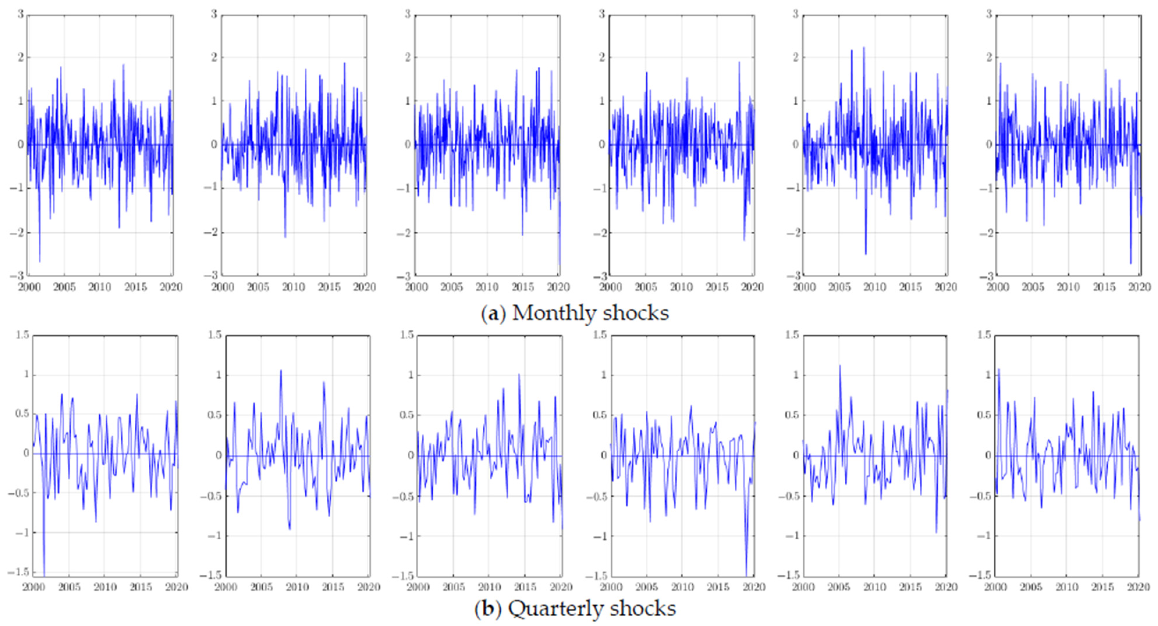
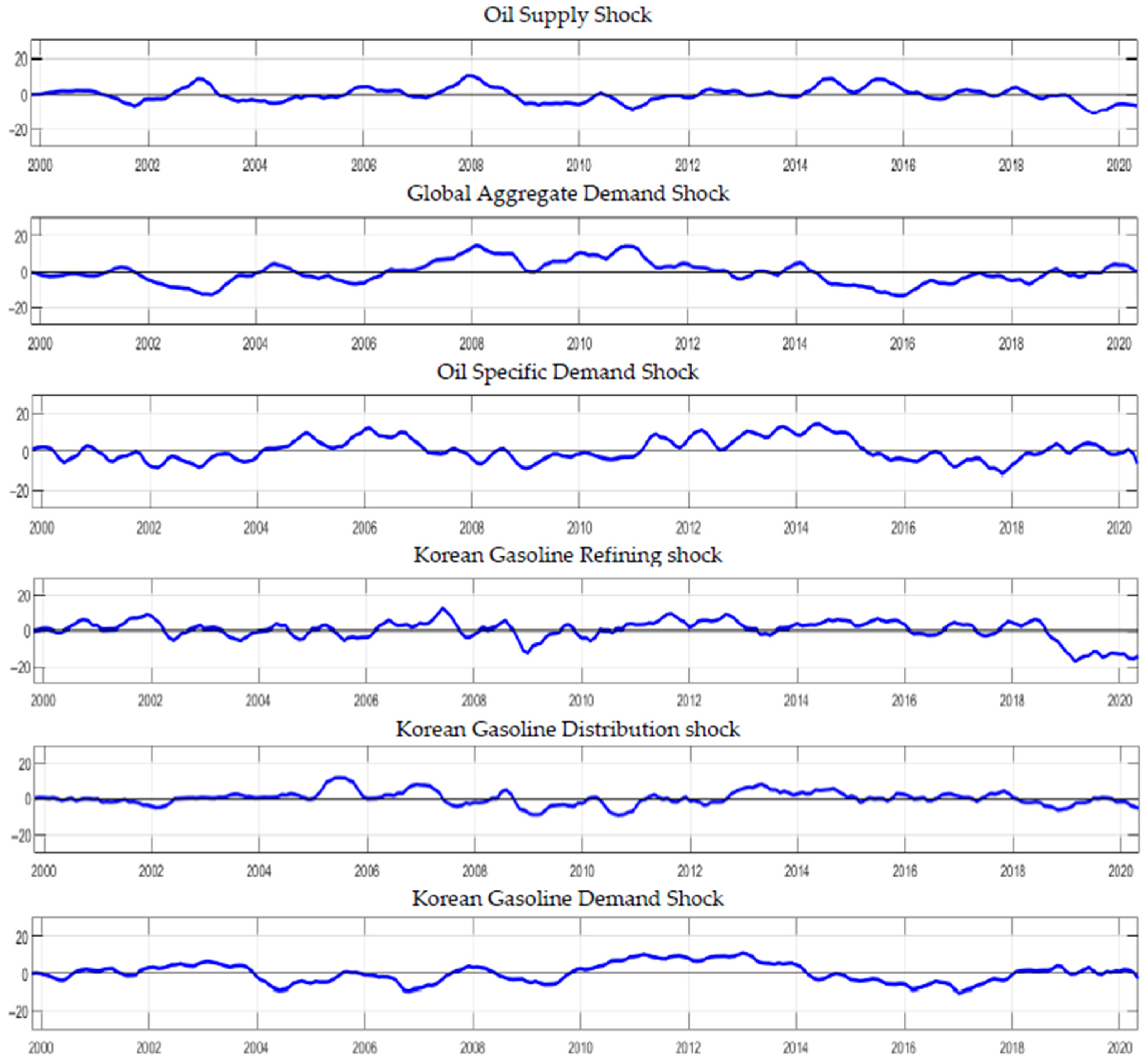
4.1. Decomposition of Structural Oil Price Shock Factors

The six shocks decomposed based on the model and data constructed in Section 3 are shown in Figure 2. The identified e t , which are the impact paths for each period of six structural shocks during the analysis period, is shown. To this end, the monthly shock is the basic shock identified in the original data, and the shock converted by the quarterly average of the monthly shock is the quarterly shock.

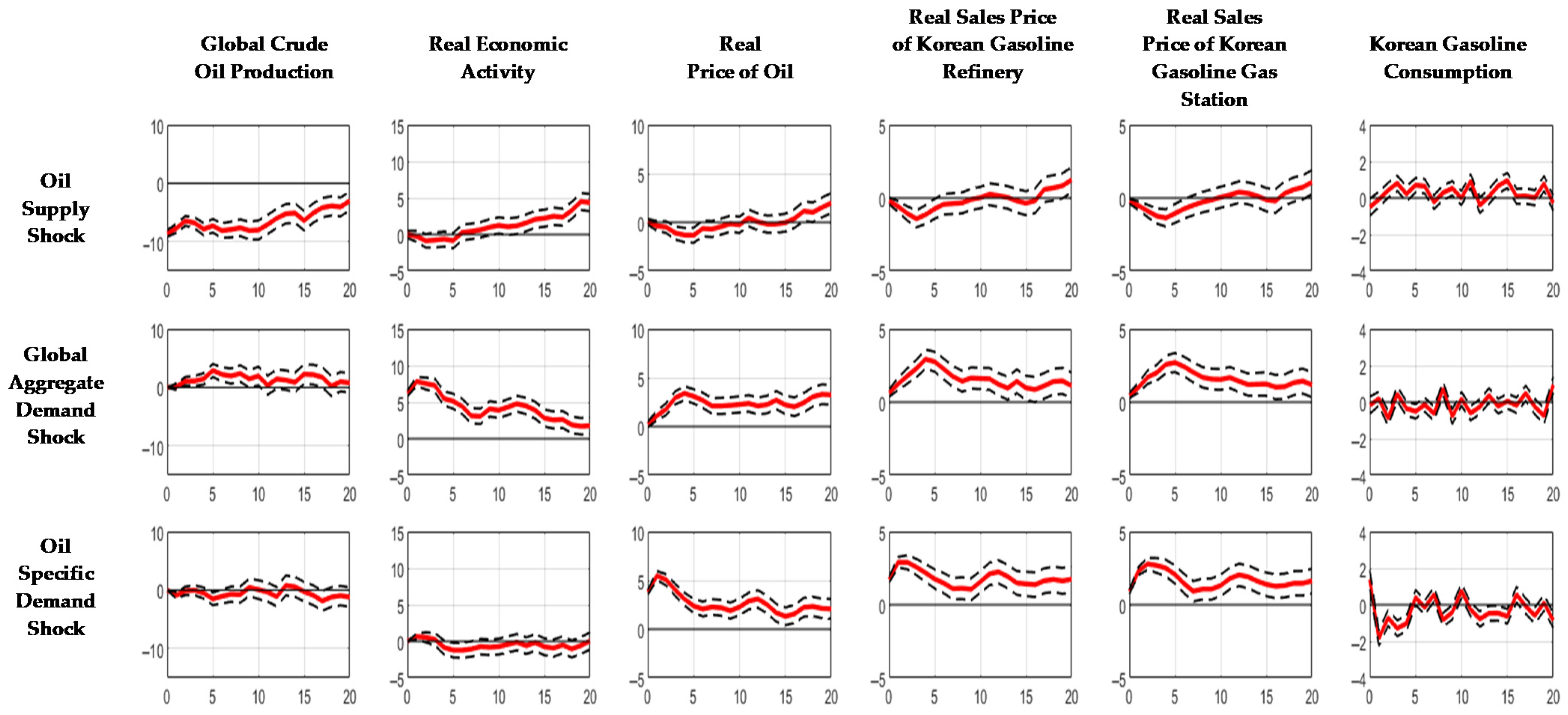
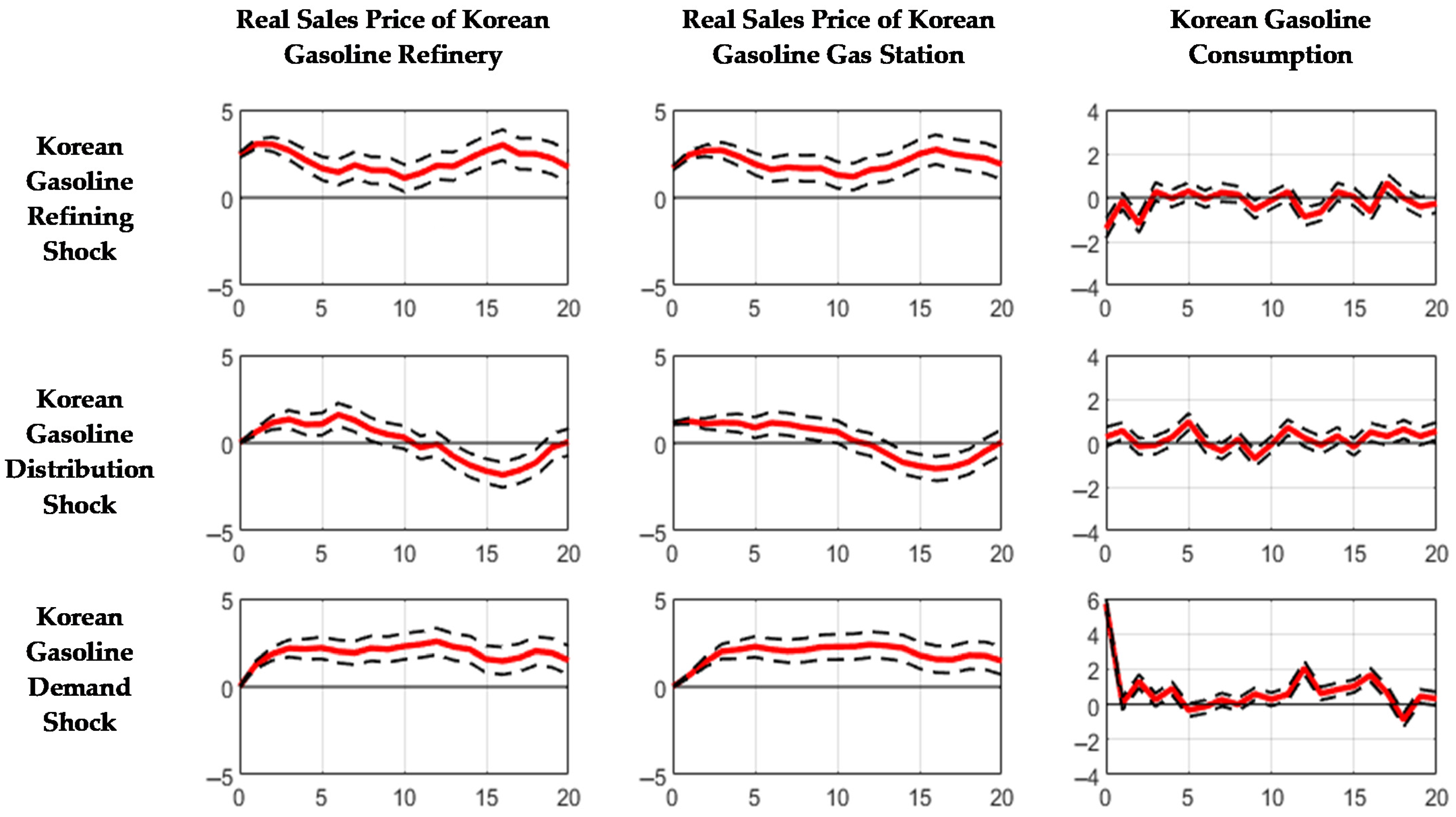
4.2. Impulse Response Analysis in the Global Crude Oil Market and Korean Gasoline Market

In this section, the impulse response analysis is conducted to see the effect of the six on the GCO market and KG market when six shocks occur virtually, targeting these variables. In the case where each shock occurs as much as 1-SD, the monthly impulse response analysis is performed, and the impulse response lag is set to 20 months. To induce an increase in GCO and KG prices, the other shocks, except for the oil supply shock, are designed toward increasing the shock. In the case of the oil supply shock, a negative shock is used to set the direction in which oil prices rise due to confusion and a decrease in crude oil supply. Figure 3 shows the results of the impulse response analysis of six variables to the three shocks in the GCO market.
In Figure 3, the oil supply shock has a significant negative effect on crude oil production in the early stage. However, the influence gradually decreases, showing a partial recovery around 12 months and a complete recovery after 20 months. This is consistent with the view that the reduction of oil supply in one region tends to stimulate production in another region. Therefore, the disruption in crude oil production caused by the oil supply shock does not cause supply problems in the long term. Next, the oil supply shock initially slightly reduces the real economic activity due to the reduction of crude oil production, but it shows the recovery of real economic activity after approximately six months with the recovery of crude oil production.
The fact that the real economic activity rises after a certain point despite the oil supply shock is contrary to the usual economic logic. However, a structural change may occur as the analysis period has expanded since 2010, along with the fact that crude oil production rapidly recovers in the short term due to the oil supply shock. In other words, the impact of the oil supply shock on real economic activity may have decreased. Indeed, the result was a slight increase in real economic activity due to the oil supply shock in Kang et al. (2019), who extended the analysis period until June 2016 [15]. As seen in previous studies, various documents have pointed out that the influence of oil price shock is decreasing compared to the past due to the decline in the dependence on oil in the economy, the increase in wage elasticity in the labor market, changes in the economic structure, and the promotion of the role of monetary policy. Inferring from the same context, we can interpret that the impact of the oil supply shock has decreased compared to the past, resulting in a rapid recovery of crude oil production and real economic activity in the short term.
The oil supply shock does not have a significant effect on real oil prices, despite a decrease in crude oil production. An interesting point is the fact that the influence on oil prices shows a pattern similar to fluctuations in real economic activity. That is, the real price of oil decreases slightly as the real economic activity initially decreases due to the oil supply shock, and the real price of oil also rises again similarly with some lags from the time when the real economic activity recovers. By contrast, we cannot easily say that a decrease in crude oil production directly increases the real price of oil. This fact is somewhat similar to Kilian (2009) [14]. The oil supply shock does not have a significant effect on the real price of oil; thus, it does not significantly affect the two types of real sales prices of KG. Both gasoline prices decline slightly before eight months and slightly increase after 16 months; however, its relevance in terms of size and standard error cannot be assured. Finally, the oil supply shock does not cause any significant decreases in KG consumption.
The global total demand shock, which reflects the global demand for industrial goods as a whole, increases the crude oil production slightly and real economic activity hugely for more than 20 months. Especially, the synergistic effect of real economic activity is large at the beginning and gradually decreases, but the effect lasts for more than 20 months. Therefore, it causes a significant continuous increase in the real price of oil for more than 20 months because it induces a greater increase in real economic activity than the increase in crude oil production. Accordingly, the significant rise in the real price of oil results in a significant increase in both types of KG prices. At this point, the effects of increasing two KG prices peak in the fourth month, and then gradually decrease, unlike the real price of oil. Despite the continuous rise in the real price of oil and two real sales prices of KG, the effect is weak on KG consumption. The fact that KG consumption does not change significantly despite rising prices is considered to be related to its inelasticity. According to Lim (2009), gasoline consumption is inelastic to price changes as gasoline became a necessary good in Korea [22]. In addition to this factor, the large increase in real economic activity caused by the global total demand shock may offset the decline in KG consumption.
Finally, the oil-specific demand shock reflecting speculative or preliminary demand in the crude oil market does not have a significant effect on crude oil production and real economic activity. The oil-specific demand shock in the crude oil market reflects the expectations of market participants; hence, expectedly, there will be no significant impact on the real economy. Despite the absence of a significant impact on real economic activity and crude oil production, the oil-specific demand shock causes the largest increase in the real price of oil among the three shocks in the GCO market. In particular, the real price of oil increases hugely at the beginning, and the synergistic effect gradually decreases after that. Nevertheless, it lasts for more than 20 months. The fact that the oil-specific demand shock largely increases the real price of oil in the short term is consistent with Kilian (2009, 2010), and Kang et al. (2019) [12,14,15]. In summary, the factor that has the greatest influence on the real price of oil in the GCO market is the expectations of market participants such as speculative demand or preliminary demand. In addition, the oil-specific demand shock causes the two real prices of KG to increase significantly as well along with the huge rise in real oil price. Like the rise in the real price of oil, a large synergistic effect appears at the beginning and gradually decreases after that, but the price increase effect lasts for more than 20 months. Unlike the global total demand shock, KG consumption slightly declines in the short term for approximately six months due to the biggest rise in the real price of oil and two real prices of KG. This also shows a short-term recovery due to the inelasticity of KG consumption.
As a result, the two demand-side factors cause the biggest increase in the real price of oil and two real gasoline prices in Korea. In addition, the oil-specific demand shock in the crude oil market can be confirmed as the most significant factor affecting KG consumption.
Next, Figure 4 shows the results of the impulse response analysis of the three variables to the three shocks in the KG market. Here, the reactions to the GCO market are excluded based on the assumption that shocks from the KG market cannot affect the GCO market due to the Korean economic structure and scale.
The KG-refining shock caused by an unexpected increase in refining costs or confusion in refining facilities significantly increases the two kinds of gasoline prices constantly for more than 20 months. When refining costs increase due to an unexpected accident in the refining operation facility, refiners have no choice but to reduce gasoline supply in the short term, resulting in a considerable initial price increase. In addition, as the price increase effect continues, the occurrence of trouble in the refinery operation facility may recover in the short term. In the case of Korea, four representative companies in the oil refining industry occupy a large part of the market, so each oil refining company has a large proportion of the total domestic volume. Accordingly, if at least one company has a problem with the refining operation facility, the price increase effect is inevitable and long-term, unless other companies increase the quantity sufficiently. Finally, the KG refining shock also initially reduces KG consumption slightly for about four months, but it recovered quickly just like the oil-specific demand shock in the crude oil market.
Meanwhile, the KG distribution shock slightly increases two types of gasoline prices for approximately 10 months, and its size is not that great compared to other shocks. Although the price has recovered as it enters a negative shock after 10 months, this is somewhat intuitive. When the selling price of gasoline gas stations rises due to a sudden increase in distribution costs, consumers are likely to try searching for relatively cheap gas stations. Accordingly, gas stations are highly likely to find relatively inexpensive wholesale suppliers rapidly to lower the price or to keep prices low even at the cost of a loss. These factors seem to restore the price increase caused by the distribution shock in the short run. The price increase effect caused by the KG distribution shock is small and short term; therefore, it does not cause any significant fluctuations in KG consumption.
Lastly, the KG demand shock increases KG consumption largely at an early phase. The increased effect of gasoline consumption converges to zero in the very short run. This is also considered to be related to the inelasticity of KG consumption. However, the large ascending effect on the two selling prices lasts for more than 20 months due to the rapid increase in consumption in the early stage.
In summary, among the three shocks in the KG market, the KG-refining shock and KG demand shock are the factors that continuously and greatly increase the two KG prices. However, the impact of the distribution shock was relatively small and short-term. This fact suggests that the impact of wholesale supply along with the influence of demand is important in the price fluctuations of the KG market.

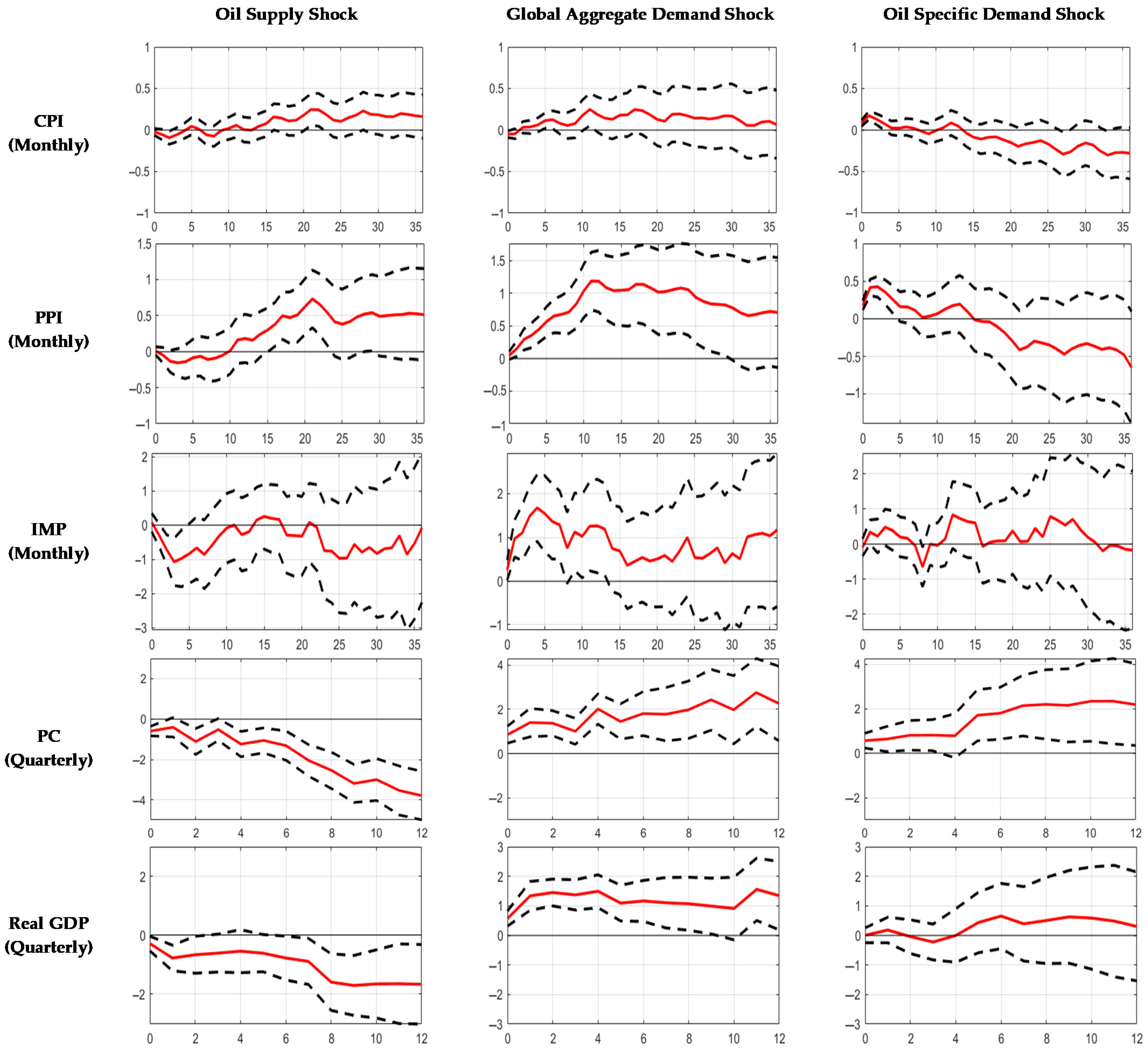
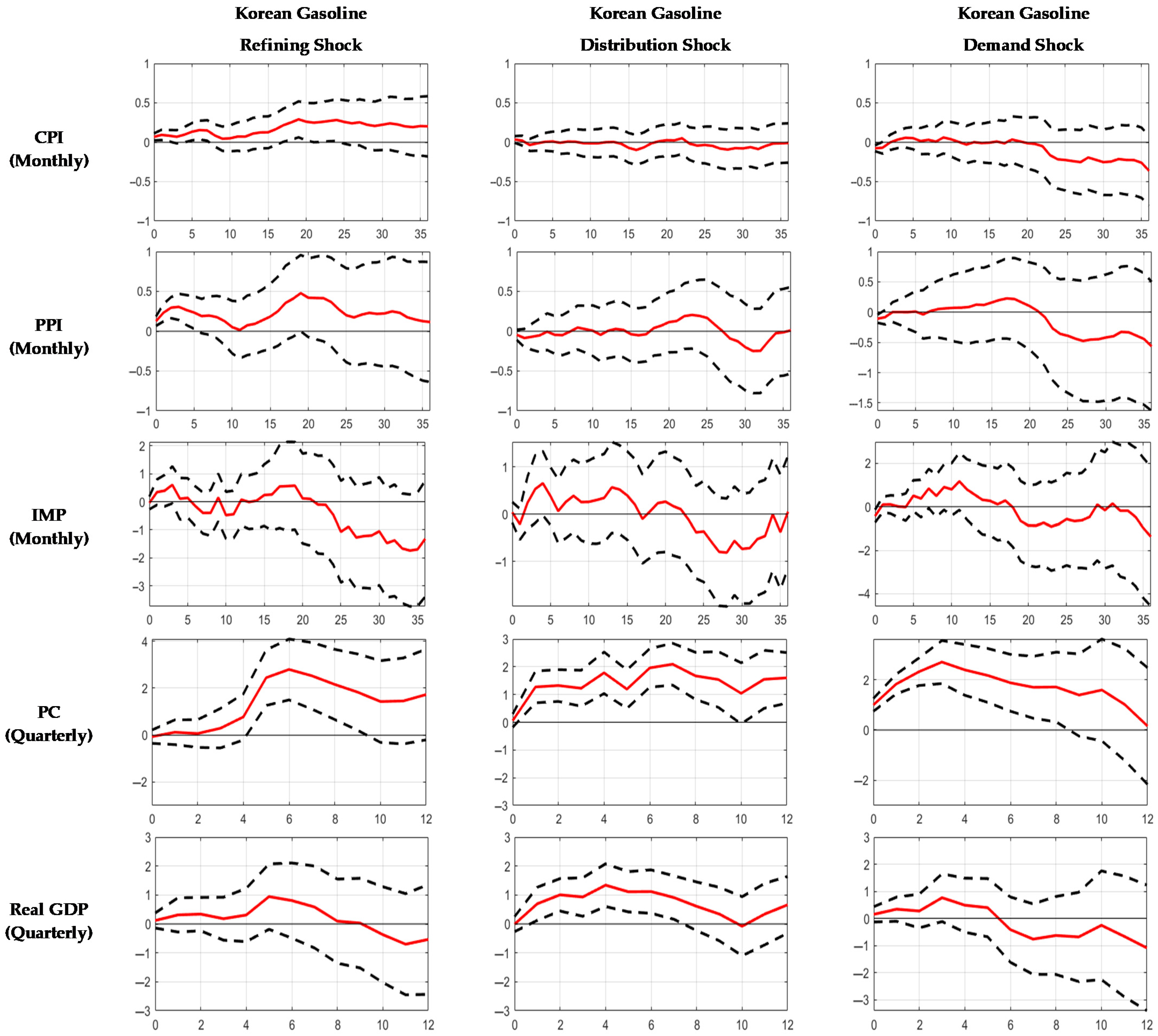
4.3. Effect of Structural Oil Price Shock Factors on the Macroeconomy

In this section, impulse response analysis is conducted to examine how each shock affects the overall macroeconomy in Korea. When each shock increases by 1-SD (Standard Deviation) virtually, impulse response analysis on major macro-variables is performed. The previously decomposed six shocks are pre-determined.
Based on the previously identified shocks, the models for performing the impulse response analysis on monthly and quarterly macro-variables are as shown in Equations (5) and (6).
M t = a j + i = 0 36 φ j i e j , t i ^ + v j t ,   j = 1 , 2 , 3 , 4 , 5 , 6
Q t = b j + i = 0 12 ψ j i u j , t i ^ + w j t ,   j = 1 , 2 , 3 , 4 , 5 , 6
In Equation (5), e j , t i ^ stands for the previously identified monthly structural shocks, and v j t represents the structural disturbance terms of each shock. j = 1, 2, 3, 4, 5, 6 are oil supply shock, global total demand shock, oil-specific demand shock, KG-refining shock, KG distribution shock, and KG demand shock, respectively. φ j i denotes the impulse response coefficient of each shock by lag, and macro-variables with monthly data are entered as the dependent variable M t . In this case, impulse response analysis for macro-variables is performed using a 36-month lag.
Next, to analyze the variables with quarterly data, we use quarterly shocks u j , t i ^ converted from monthly shocks into quarterly averages. Based on the converted quarterly shocks, the model set up to conduct impulse response analysis for variables with quarterly data is Equation (6). ψ j i is the impulse response coefficient of each quarterly shock, and macro-variables quarterly data are input as the dependent variable Q t in Equation (6). The time lag is set to 12 quarters, the same as the monthly impulse response analysis.
Table 1 summarizes the macroeconomic variables in Korea used in the analysis.
Figure 5 shows the impulse response analysis results of five macro-variables for the three shocks in the GCO market. As before, only the case of rising prices is considered. Falls in gasoline and oil prices are excluded from the analysis, at least on the assumption that they do not negatively affect the macroeconomy.
Looking at Figure 5, we can see that the rise in oil prices resulting from the oil supply shock causes stagflation for three years as the import price of crude oil rises without any offsetting factors. This increases the CPI and the PPI for more than three years. In the event of the oil supply shock, the CPI increases by 0.16% cumulatively over three years. The PPI increases by 0.51% cumulatively over three years, but it has not been statistically significant since 20 months. At this time, the rise in international oil prices and KG prices is not that large, so inflation is not as huge as the global aggregate demand shock (Figure 3). In addition, oil supply shock is shown to generally reduce manufacturing production (IMP) even if it is not statistically significant, and significantly reduces private consumption (PC) for three years. Without an offsetting factor through the demand-side, an increase in oil prices and inflation simply act as a burden on the manufacturing industry, resulting in a contraction of the manufacturing industry. Particularly, private consumption decreases by 3.78% cumulatively over three years. This is interpreted because no positive factor exists to support private consumption, and only inflation occurs. Consequently, a decline in private consumption and a modest reduction in manufacturing production cause real gross domestic product (GDP) to reduce to 1.67% cumulatively. This result is consistent with the view of Peersman and Van Robays (2009, 2012), who argued that oil price shocks caused by supply shock induce stagflation pressure in the long term in crude oil importing countries [18,19].
Meanwhile, an increase in oil prices caused by the global aggregate demand shock and the oil-specific demand shock in the crude oil market does not cause stagflation. In the case of the global aggregate demand shock, the CPI and the PPI increase due to the burden of significant increases in the real price of oil and gasoline, and the dramatic rise in real economic activity (Figure 3). Although the CPI has been shown to increase slightly, it has been difficult to obtain statistical significance for about 15 months. Meanwhile, the PPI rises the most among the three shocks of the GCO market. The global aggregate demand shock raises the PPI by 1.19% significantly over 12 months, and the effect gradually decreases after that. Consequently, it increased by 0.7% over three years cumulatively, but this result was not statistically significant. Despite the slight increase in the CPI and the large increase in the PPI, the rapid rise in real economic activity caused by an increase in global aggregate demand generally increases the index of manufacturing production by 1.18% for three years although it has been difficult to obtain statistical significance since about 12 months. It raises private consumption 2.26% cumulatively for three years. Notably, even in the manufacturing industry, which is sensitive to rising oil prices, the increase in global aggregate demand offsets the negative effects of rising oil prices, thereby boosting manufacturing production. As a result, despite the inflation and increase in oil prices, the global aggregate demand shock increases the real GDP by 1.34%.
Rising oil prices due to an unexpected increase in preliminary or speculative demand in the crude oil market initially increase the CPI and PPI. The CPI rises 0.12% in the first month, but the effect continues to decline after that, reaching the same level as before the shock after 13 months. Consequently, the CPI cumulatively decreases by 0.28% after three years. Similarly, the PPI rises to 0.42% in the second month. However, like the CPI, the effect continues to decline, reaching the same level as before the shock in the 15 months. As a result, the PPI decreases by 0.65% cumulatively over three years, but this result was not statistically significant. This is related to a strong increase in oil and gasoline prices in the short term due to the oil-specific demand shock, and the effect gradually disappears. Both indexes consequently decrease after a certain time, which does not cause any significant change in manufacturing production. The oil-specific demand shock has been shown to have a non-significant effect on IMP. In addition, this fact causes the effect of vitalizing private consumption for three years. However, the real GDP is shown to slightly increase to 0.3% over three years but is generally insignificant.
In summary, the oil supply shock harms the Korean macroeconomy; however, the negative effect of the two demand-side factors is hard to determine. An interesting point in Figure 5 is the fact that the PPI responds more to the three shocks in the GCO market than the CPI. This result means that regardless of the impact factor, the oil price shock acts as a greater burden on the companies in the first transaction stage due to the increase in production cost than the consumers who consume the final goods. This result is similar to that of Cha and Oh (2014) [77].
Next, Figure 6 shows the impulse response analysis results of five macrovariables for the three shocks in the KG market.
The rise in gasoline-refining costs in Korea due to unexpected problems with refining operation facilities also causes problems in the supply of gasoline, resulting in the rise in CPI and PPI for more than three years. The gasoline-refining shock increases the CPI by 0.2%, accumulated over three years. In addition, this shock is shown to raise the PPI for three years but is not statistically significant. The rise in domestic gasoline prices and two some inflation indices put a burden on the manufacturing industry, and this effect begins in earnest after 21 months. The manufacturing production index, which begins to decline in earnest after 21 months, eventually decreases by 1.31% over three years. Contrary to expectations, the rise in gasoline prices due to refining shocks does not adversely affect private consumption. It will be mentioned later through comparison with other gasoline-related shocks, but unlike crude oil price shocks, gasoline price shocks do not appear to harm private consumption overall. The price shock in the domestic gasoline market does not seem to hurt the total amount of private consumption. As shown in Figure 4, this is interpreted to be related to a short-term settlement to the reduction in gasoline consumption as gasoline becomes an inelastic commodity despite rising gasoline prices. Despite the decline in manufacturing production after a certain point, the real GDP does not decrease until the 9 quarters, as private consumption is not affected much. However, as the production decline in the manufacturing industry intensifies, the real GDP also declines. However, its cumulative 0.54% decrease is less than that in the manufacturing production index due to the influence of private consumption, and this is also hard to say meaningful. As a result, the KG-refining shock causes some stagflation eventually, but this is not obvious.
Meanwhile, the negative impact of the KG distribution shock on the macroeconomy is not significant. Increasing gasoline distribution costs due to unexpected problems in the distribution process or exceeding the distribution limit does not cause significant fluctuations in the CPI and PPI. In the case of manufacturing production, a slight decrease is shown after 22 months, but this decrease may not be significant in terms of the coefficient value and standard error. In addition, even this part, which has decreased slightly, has recovered rapidly. As a result, no significant change occurs in the manufacturing production index cumulatively. Meanwhile, private consumption does not decrease as with other gasoline-related shocks, and real GDP rises slightly based on private consumption. Due to the gasoline distribution shock in Korea, real GDP rises by 1.34% for the four quarters, and 0.66% cumulatively for threee years. The fact that the KG distribution shock does not harm the macroeconomy is related to the point that the gasoline price increase effect is very small and is resolved in the short term (Figure 4).
Lastly, the gasoline demand shock in Korea does not seem to cause many fluctuations in the CPI and PPI. Although it is not statistically significant, CPI and PPI have been shown to decrease since a certain point. This seems to be related to the extremely short-term recovery of consumption growth caused by gasoline demand shock (Figure 4). Despite the short-term increase in gasoline demand, gasoline prices continue to rise. Therefore, the burden of this eventually decreases demand for other goods, which in turn leads to some deflation after a certain point. As gasoline consumption increases initially due to gasoline demand increases, private consumption increases sharply, accumulating up to 2.7% until quarter 3. The manufacturing production index also increases by 1.17% up to 11 months due to the increase in gasoline demand. However, the effects of the two macro-variables begin to reduce gradually because of the short-term recovery of gasoline consumption and the burden of high gasoline prices. As a result, private consumption increases by 0.16% cumulatively over three years due to the disappearance of the effect of increasing private consumption, and the manufacturing production index decreases by 1.37% cumulatively over three years. However, it is difficult to see a clear reduction in IMP, given that the decrease in IMP is not statistically significant. Accordingly, the real GDP also shows a slight increase until the fifth quarter owing to the large increase in private consumption and the modest increase in the manufacturing production index at the beginning. However, after that, it decreases due to a decrease in private consumption and the manufacturing production index, and cumulatively decreases by 1.09% for 3 years. The gasoline demand shock reduces the real GDP after 5 quarters, but it was not statistically obvious. As a result, its stagflation effect is uncertain because it does not cause definite inflation and an obvious reduction of real GDP.

4.4. Historical Contribution to the Gasoline-Selling Price in Korea

This section examines how historically the six shocks of the GCO market and the KG market contributed to the selling price of gasoline stations in Korea through historical decomposition. Figure 7 shows the historical decomposition results for the real selling price of gasoline stations in Korea.
As shown in Figure 7, among the three shocks of the GCO market, the oil supply shock contributed relatively little to the fluctuations in gasoline prices in Korea since the 2000s. The oil supply shock caused gasoline prices to rise four times since the 2000s, but it did not cause long-term price fluctuations. By contrast, the global aggregate demand shock and the oil-specific demand shock contributed relatively significantly to fluctuations in gasoline prices in Korea. Next, among the three shocks in the KG market, the gasoline demand shock historically contributed the most to the fluctuations in gasoline prices in Korea. Meanwhile, KG refining shock and distribution shock also caused significant price fluctuations, but it was not lasting and played a role in partially amplifying or offsetting price fluctuations caused by other shocks like the oil supply shock.
Looking at Figure 7 divided by period, from 2001 to early 2004, we can see that small-scale oil supply shock, refining shock, and KG demand shock acted as factors to increase prices, but the level of gasoline prices was lower than the average due to relatively strong negative global aggregate and oil-specific demand shocks in the crude oil market. After that, the strong positive (+) oil-specific demand shock from 2004 led to a rise in gasoline prices. Moreover, one refining shock and two gasoline distribution shock also partially contributed to the price increase in the short term. Around 2007, the impact of oil-specific demand shocks in the crude oil market slightly declined, acting as a factor in lowering gasoline prices. However, KG prices rose to 1922 won per liter in July 2008 because of the rapid increase in global aggregate demand and short-term oil supply decline factors. Since then, with the arrival of the global financial crisis, the price of gasoline in December 2008 recorded 1329 won per liter, as all other shocks acted as factors that lowered prices along with a decrease in global aggregate demand.
Since then, the sharp decline in gasoline prices gradually recovered due to the recovery of global demand and maintained a high gasoline price level due to the impact of strong positive oil-specific and KG demand shocks. In 2012, the price of gasoline reached more than 2000 won per liter, and the high level of more than 1800 won per liter continued until the end of 2014. Since 2015, a slight oil supply shock acted as a price increase factor, but prices maintained at a low level due to the negative global aggregate, oil-specific, and KG demand shocks. Lastly, the rapid decline in gasoline prices in early 2020 was driven by an oversupply of crude oil that began in 2019, a decrease in gasoline-refining costs, or an excessive number of refining facilities. At this time, a slight negative oil-specific demand shock and distribution shock are observed, but its significance is uncertain because it is observed at the end of the time series.
Hence, Figure 7 shows that the global aggregate, oil-specific, and KG demand shocks have been the most major factors in the volatility of gasoline prices in Korea since the 2000s, excluding 2020. In addition, the oil supply shock, KG-refining shock, and KG distribution shock were small and short-term shocks, but they partially caused significant fluctuations.

5. Discussion and Conclusions

This study used the SVAR model to identify six structural shock factors (oil supply shock, global aggregate demand shock, oil-specific demand shock, KG-refining shock, KG distribution shock, and KG demand shock). Based on this, when each shock occurs virtually, we examined the effects on the variables of the KG market and the GCO market, as well as the effects on the major variables of the macroeconomy in Korea. This paper also looked at how the six shocks have historically contributed to gasoline prices in Korea.
The analysis results confirmed that when the six shock factors virtually occurred, the effects on the KG market, the GCO market, and major variables of the macroeconomy in Korea were different. Among the three shocks in the GCO market, the oil supply shock did not have a great influence on real oil and gasoline prices in Korea, but it caused stagflation and contraction in manufacturing and private consumption. By contrast, the two demand-side factors in the GCO market had a relatively large influence on real oil prices and KG prices. Excluding inflation, we determined that the global aggregate demand shock produced a positive response to the economy as a whole. Moreover, the oil-specific demand shock in the crude oil market was smaller or insignificant than the global aggregate demand shock, but it also produced positive or at least not negative results in general.
Meanwhile, among the three shocks in the gasoline market in Korea, the KG refining shock had a lasting effect on the gasoline price and caused some stagflation and manufacturing contraction after a certain point. However, it was not as strong as the oil supply shock and was not statistically significant. Likewise, the KG demand shock continued to increase the gasoline price, and it caused an economic recession and a contraction in the manufacturing industry after a certain point. However, this was also unclear and insignificant. This shock did not increase inflation obviously and decrease private consumption. Lastly, the distribution shock in the KG market had a short-term increase effect in gasoline prices and did not negatively affect the economy. Consequently, the oil price shock cannot be said to simply harm the macroeconomy. Moreover, the influence of complex factors, including the shocks in the domestic gasoline market, needs to be examined comprehensively and in detail.
In particular, according to the historical decomposition analysis results, the influence of the two demand-side factors is more important historically than the oil supply shock in gasoline price fluctuations in Korea, and the KG demand shock is the most important in the KG market. From the fact that the global aggregate, oil-specific, and KG demand shocks are those that have contributed the most to the rise in gasoline prices in Korea since the 2000s, it cannot be concluded that the rise in oil and gasoline prices negatively affected the domestic macroeconomy. These results follow previous studies suggesting a problem in interpreting oil price shocks by simply limiting them to an exogenous oil supply shock. In addition, the fact that the influence of refining shock and distribution shock in gasoline price fluctuations was also partly significant historically suggests the necessity to analyze the oil price shock in connection with the domestic gasoline market by decomposing factors and to confirm the influence on the macroeconomy, beyond simply analyzing the GCO market.
In Korea, claims about the necessity of a stable supply of crude oil have been continuously raised due to concerns about the oil supply problem and the economic downturn caused by oil price shocks. However, historically, the effect of crude oil supply shocks on gasoline prices in Korea was not significant. Since the 2000s, only a few cases of price increase caused by oil supply shocks have occurred, which have also been short-term. In addition to the oil supply shock, the oil price shock has various fundamental factors including demand-side factors and factors of the domestic gasoline market. These arguments lose effectiveness in that the influence of each shock is different. Rather, the fundamental factors that have changed the prices of crude oil and domestic gasoline must be checked, and the magnitude of each impact must be compared. Accordingly, the ripple effect on the macroeconomy must be predicted accurately. After that, we must pay attention to an appropriate policy suitable for the fundamental shock. For example, if there is a strong price increase due to the impact of crude oil supply in the GCO market, an expansionary monetary policy or fiscal policy may be implemented at the expense of a certain level of inflation, but if there is a strong price increase due to two other demand factors, there may be no need to respond by any policy. This process could help offset negative effects and amplify positive effects on the macroeconomy. In addition, since the 2000s, the problem of oil supply has no longer been of great importance due to the weakening dependence on crude oil globally, so trade policies focusing on oil supply are considered to be less effective. These points are necessary for policymakers to keep in mind.
There is also an additional suggestion for the KG market. In the case of KG distribution shocks, the price shocks were very weak and remained at a short-term level due to intensifying competition. On the other hand, the effect of the gasoline refining shock in Korea was relatively long-term and strong. This also showed some negative effects on the macroeconomy. The impact of this shock is attributed to the oligopoly structure of a small number of refiners in the KG market, and it is expected that this impact can be mitigated through diversification of the competitive structure. This will indirectly help the energy conversion policy in Korea to be sustainable in the future.
Nevertheless, this study has the following limitations. First, the variable used in this study has some issues. Regional differences apparently occur in the case of the sales price of KG gas stations, which are used to break down the gasoline distribution shock clear. However, the fact that regional differences were excluded using national weighted average prices to examine overall trends remains a limit. This will expectedly lead to future studies examining the differences by decomposing distribution shocks by region using regional gasoline prices. In addition, due to the absence of some data, this study has not been able to cover many data since the coronavirus period in 2020. Accordingly, the timing of the oil price collapse in early 2020 may have partially distorted the analysis. However, this can be corrected as the analysis period expands and thus becomes clearer. Finally, the lack of rigor in interpretation remains a limitation due to the insufficient papers examining the impact on macroeconomy via the domestic gasoline price shocks decomposition. We also plan to add sophistication of result interpretation through continuous research.

Author Contributions

Conceptualization, J.L. and H.C.C.; methodology, J.L. and H.C.C.; software, J.L.; validation, H.C.C.; formal analysis, J.L.; investigation, J.L.; resources, H.C.C.; data curation, H.C.C.; writing—original draft preparation, J.L. and H.C.C.; writing—review and editing, J.L. and H.C.C.; visualization, J.L.; supervision, H.C.C.; project administration, H.C.C. All authors have read and agreed to the published version of the manuscript.

Funding

This research has been done by the author(s) working at the Department of Economics at Dankook University, which was supported by the Research-Focused Department Promotion Project as a part of the University Innovation Support Program 2020 to Dankook University.

Institutional Review Board Statement

Not applicable.

Informed Consent Statement

Not applicable.

Data Availability Statement

Real Economic Activity Data, https://sites.google.com/site/lkilian2019/research/data-sets, accessed on 15 February 2020; Korean Macroeconomy Data, https://kosis.kr, accessed on 15 February 2020; Korean Gasoline Data, https://www.opinet.co.kr, accessed on 15 February 2020, https://www.petronet.co.kr, accessed on 15 February 2020.

Conflicts of Interest

The authors declare no conflict of interest.

References

  1. Van de Ven, D.J.; Fouquet, R. Historical energy price shocks and their changing effects on the economy. Energy Econ. 2017, 62, 204–216. [Google Scholar] [CrossRef] [Green Version]
  2. Zerrin, K.; Yasemin, D. Macroeconomic Impacts Of Oil Price Shocks: An Empirical Analysis Based On The Svar Models. Rev. Econ. 2017, 69, 55–72. [Google Scholar]
  3. Dramani, J.B.; Frimpong, P.B. The effect of crude oil price shocks on macroeconomic stability in Ghana. OPEC Energy Rev. 2020. [Google Scholar] [CrossRef]
  4. Almutairi, N. The effects of oil price shocks on the macroeconomy: Economic growth and unemployment in Saudi Arabia. OPEC Energy Rev. 2020, 44, 181–204. [Google Scholar] [CrossRef]
  5. Borenstein, S.; Cameron, A.C.; Gilbert, R. Do gasoline prices respond asymmetrically to crude oil price changes? Q. J. Econ. 1997, 112, 305–339. [Google Scholar] [CrossRef]
  6. Manning, D.N. Petrol price, oil prices rises and oil price falls: Evidence for the UK since 1972. Appl. Econ. 1991, 23, 1535–1541. [Google Scholar] [CrossRef]
  7. Kaufmann, R.K.; Laskowski, C. Causes for an asymmetric relation between the price of crude oil and refined petroleum products. Energy Policy 2005, 33, 1587–1596. [Google Scholar] [CrossRef]
  8. Radchenko, S.; Shapiro, D. Anticipated and unanticipated effects of crude oil prices and gasoline inventory changes on gasoline prices. Energy Econ. 2011, 33, 758–769. [Google Scholar] [CrossRef]
  9. Kuper, G.H. Inventories and upstream gasoline price dynamics. Energy Econ. 2012, 34, 208–214. [Google Scholar] [CrossRef]
  10. Polemis, M.L.; Fotis, P.N. The taxation effect on gasoline price asymmetry nexus: Evidence from both sides of the Atlantic. Energy Policy 2014, 73, 225–233. [Google Scholar] [CrossRef]
  11. Hong, W.; Lee, D. Asymmetric pricing dynamics with market power: Investigating island data of the retail gasoline market. Empir. Econ. 2018, 58, 2181–2221. [Google Scholar] [CrossRef]
  12. Kilian, L. Explaining fluctuations in gasoline prices: A joint model of the global crude oil market and the U.S. retail gasoline market. Energy J. 2010, 31, 87–112. [Google Scholar] [CrossRef] [Green Version]
  13. Edelstein, P.; Kilian, L. How sensitive are consumer expenditures to retail energy prices? J. Monet. Econ. 2009, 56, 766–779. [Google Scholar] [CrossRef]
  14. Kilian, L. Not all oil price shocks are alike: Disentangling demand and supply shocks in the crude oil market. Am. Econ. Rev. 2009, 99, 1053–1069. [Google Scholar] [CrossRef] [Green Version]
  15. Kang, W.; Perez de Gracia, F.; Ratti, R.A. The asymmetric response of gasoline prices to oil price shocks and policy uncertainty. Energy Econ. 2019, 77, 66–79. [Google Scholar] [CrossRef]
  16. Lippi, F.; Nobili, A. Oil and the macroeconomy: A quantitative structural analysis. J. Eur. Econ. Assoc. 2012, 10, 1059–1083. [Google Scholar] [CrossRef] [Green Version]
  17. Baumeister, C.; Peersman, G. Time-varying effects of oil supply shocks on the US economy. Am. Econ. J. Macroecon. 2013, 5, 1–28. [Google Scholar] [CrossRef] [Green Version]
  18. Peersman, G.; Van Robays, I. Oil and the Euro area economy. Econ. Policy 2009, 24, 603–651. [Google Scholar] [CrossRef]
  19. Peersman, G.; Van Robays, I. Cross-country differences in the effects of oil shocks. Energy Econ. 2012, 34, 1532–1547. [Google Scholar] [CrossRef] [Green Version]
  20. Kim, D.; Lee, J. Spatial Price Competition in the Korean Retail Gasoline Market. Environ. Resour. Econ. Rev. 2014, 23, 553–581. [Google Scholar] [CrossRef] [Green Version]
  21. Kim, T. Price Competition and Market Segmentation in Retail Gasoline: New Evidence from South Korea. Rev. Ind. Organ. 2018, 53, 507–534. [Google Scholar] [CrossRef]
  22. Lim, S.S. Does the government have to increase the flexible tax rate on gasoline to stabilize gasoline price in Korea? J. Consum. Policy Stud. 2009, 36, 43–66. [Google Scholar]
  23. Hamilton, J.D. Oil and the macroeconomy since World War II. J. Political Econ. 1983, 91, 228–248. [Google Scholar] [CrossRef]
  24. Mork, K.A. Oil and the macroeconomy when prices go up and down: An extension of Hamilton’s results. J. Political Econ. 1989, 97, 740–744. [Google Scholar] [CrossRef]
  25. Lee, K.; Ni, S.; Ratti, R.A. Oil shocks and the macroeconomy: The role of price variability. Energy J. 1995, 16, 39–56. [Google Scholar] [CrossRef] [Green Version]
  26. Hamilton, J.D. This is what happened to the oil price-macroeconomy relationship. J. Monet. Econ. 1996, 38, 215–220. [Google Scholar] [CrossRef]
  27. Hamilton, J.D. What is an oil shock? J. Econ. 2003, 113, 363–398. [Google Scholar] [CrossRef]
  28. Balke, N.S.; Brown, S.P.A.; Yucel, M.K. Oil price shocks and the U.S. economy: Where does the asymmetry originate? Energy J. 2002, 23, 27–52. [Google Scholar] [CrossRef] [Green Version]
  29. Cunado, J.; Pérez de Gracia, F. Do oil price shocks matter? Evidence for some European countries. Energy Econ. 2003, 25, 137–154. [Google Scholar] [CrossRef] [Green Version]
  30. Edelstein, P.; Kilian, L. The response of business fixed investment to changes in energy prices: A test of some hypotheses about the transmission of energy price shocks. B.E. J. Macroecon. 2007, 7, 7. [Google Scholar] [CrossRef]
  31. Kilian, L.; Vigfusson, R.J. Are the responses of the U.S. economy asymmetric in energy price increases and decreases? Quant. Econ. 2011, 2, 419–453. [Google Scholar] [CrossRef] [Green Version]
  32. Kilian, L.; Vigfusson, R.J. Nonlinearities in the oil price-output relationship. Macroecon. Dyn. 2011, 15, 337–363. [Google Scholar] [CrossRef] [Green Version]
  33. Lee, K.; Jeong, H. An effect of oil price increase on the national income, inflation and monetary policy. RFE 2002, 16, 103–130. [Google Scholar]
  34. Kim, K.S. Asymmetric impacts of international oil shocks on domestic growth rate and Inflation. EAER 2005, 9, 175–211. [Google Scholar] [CrossRef]
  35. Kim, K.S. Are Korean recessions affected by oil price shocks? Econ. Anal. 2011, 17, 90–123. [Google Scholar]
  36. Cha, K. Accounting for crude oil prices: A historical decomposition. KEER 2008, 7, 1–26. [Google Scholar]
  37. Kim, K.; Yun, S. Asymmetric and nonlinear effects of oil price and exchange rate shocks on consumer price. Int. Econ. J. 2009, 15, 131–152. [Google Scholar]
  38. Kim, K. Oil price shocks and the macroeconomic activity: Analyzing transmission channels using the new Keynesian structural model. Econ. Anal. 2012, 18, 1–29. [Google Scholar]
  39. Bernanke, B.S.; Gertler, M.; Watson, M.; Sims, C.A.; Friedman, B.M. Systematic monetary policy and the effects of oil price shocks. Brook. Pap. Econ. Act. 1997, 1997, 91–142. [Google Scholar] [CrossRef] [Green Version]
  40. Barsky, R.B.; Kilian, L. Do we really know that oil caused the great stagflation? A monetary alternative. NBER Macroecon. Annu. 2001, 16, 137–183. [Google Scholar] [CrossRef]
  41. Barsky, R.B.; Kilian, L. Oil and the macroeconomy since the 1970s. J. Econ. Perspect. 2004, 18, 115–134. [Google Scholar] [CrossRef] [Green Version]
  42. Kilian, L. The economic effects of energy price shocks. J. Econ. Lit. 2008, 46, 871–909. [Google Scholar] [CrossRef] [Green Version]
  43. Segal, P. Oil price shocks and the macroeconomy. Oxf. Rev. Econ. Policy 2011, 27, 169–185. [Google Scholar] [CrossRef]
  44. Leduc, S.; Sill, K. A quantitative analysis of oil-price shocks, systematic monetary policy, and economic downturns. J. Monet. Policy 2004, 51, 781–808. [Google Scholar] [CrossRef] [Green Version]
  45. Hamilton, J.D.; Herrera, A.M. Oil shocks and aggregate macroeconomic behavior: The role of monetary policy: A comment. J. Money Credit Bank. 2004, 36, 265–286. [Google Scholar] [CrossRef]
  46. Carlstrom, C.T.; Fuerst, T.S. Oil prices, monetary policy, and counterfactual experiments. J. Money Credit Bank. 2006, 38, 1945–1958. [Google Scholar] [CrossRef]
  47. Herrera, A.M.; Pesavento, E. Oil price shocks, systematic monetary policy, and the great moderation. Macroecon. Dyn. 2009, 13, 107–137. [Google Scholar] [CrossRef] [Green Version]
  48. Lee, J.; Song, J. Nature of oil price shocks and monetary policy. In NBER Working Paper 15306; National Bureau of Economic Research, Inc.: Cambridge, MA, USA, 2009. [Google Scholar]
  49. Hooker, M.A. What happened to the oil price-macroeconomy relationship? J. Monet. Econ. 1996, 38, 195–213. [Google Scholar] [CrossRef]
  50. Blanchard, O.J.; Gali, J. The Macroeconomic Effects of Oil Price Shocks: Why Are the 2000s So Different from the 1970s? Economics Working Papers 1045, 2007; Department of Economics and Business, Universitat Pompeu Fabra: Barcelona, Spain, 2008. [Google Scholar]
  51. Dhawan, R.; Jeske, K.; Silos, P. Productivity, energy prices and the great moderation: A new link. Rev. Econ. Dyn. 2010, 13, 715–724. [Google Scholar] [CrossRef] [Green Version]
  52. Balke, N.S.; Brown, S.P.; Yucel, M.K. Oil Price Shocks and U.S. Economic Activity: An International Perspective; Working Papers 1003; Federal Reserve Bank of Dallas: Dallas, TX, USA, 2010. [Google Scholar]
  53. Caldara, D.; Cavallo, M.; Iacoviello, M. Oil price elasticities and oil price fluctuations. J. Monet. Econ. 2019, 103, 1–20. [Google Scholar] [CrossRef] [Green Version]
  54. Cha, K. A Study on the effects of oil shocks and energy efficient consumption structure with a Bayesian DSGE model. Environ. Resour. Econ. Rev. 2010, 19, 215–242. [Google Scholar]
  55. Cha, K. Time-varying effects of oil shocks on the Korean economy. Environ. Resour. Econ. Rev. 2018, 27, 495–520. [Google Scholar]
  56. Bacon, R.W. Rockets and feathers: The asymmetric speed of adjustment of UK retail gasoline prices to cost changes. Energy Econ. 1991, 13, 211–218. [Google Scholar] [CrossRef]
  57. Lee, Y.I.; Lee, J. Testing for symmetry between domestic and foreign oil price changes. Korean J. Econ. Stud. 2012, 60, 43–66. [Google Scholar]
  58. Cha, K.C. Rockets and feathers: Response of retail gasoline price to Dubai oil price changes. J. Consum. Policy Stud. 2012, 41, 67–82. [Google Scholar]
  59. Oh, S.; Choi, G.; Heo, E. A study on the asymmetry and market power in Korean petroleum products market. KEER 2015, 14, 1–25. [Google Scholar]
  60. Kim, J.W. A study on the asymmetric gasoline price response. JKOS 2017, 22, 65–91. [Google Scholar]
  61. Chang, D.; Serletis, A. Oil, uncertainty, and gasoline prices. Macroecon. Dyn. 2016, 22, 546–561. [Google Scholar] [CrossRef] [Green Version]
  62. Aloui, C.; Hkiri, B.; Nguyen, D.K. Real growth co-movements and business cycle synchronization in the GCC countries: Evidence from time-frequency analysis. Econ. Model. 2016, 52, 322–331. [Google Scholar] [CrossRef]
  63. Aloui, R.; Gupta, R.; Miller, S.M. Uncertainty and crude oil returns. Energy Econ. 2016, 55, 92–100. [Google Scholar] [CrossRef] [Green Version]
  64. Bekiros, S.D.; Gupta, R.; Paccagnini, A. Oil price forecastability and economic uncertainty. Econ. Lett. 2015, 132, 125–128. [Google Scholar] [CrossRef] [Green Version]
  65. Li, S.; Linn, J.; Muehlegger, E. Gasoline taxes and consumer behavior. Am. Econ. J. Econ. Policy 2014, 6, 302–342. [Google Scholar] [CrossRef] [Green Version]
  66. Van Robays, I. Macroeconomic uncertainty and oil price volatility. Oxf. Bull. Econ. Stat. 2016, 78, 671–693. [Google Scholar] [CrossRef]
  67. Maghyereh, A.I.; Awartani, B.; Bouri, E. The Directional Volatility Connectedness between Crude Oil and Equity Markets: New Evidence from Implied Volatility Indexes. Energy Econ. 2016, 57, 78–93. [Google Scholar] [CrossRef] [Green Version]
  68. Silvapulle, P.; Smyth, R.; Zhang, X.; Fenech, J.P. Nonparametric Panel Data Model for Crude Oil and Stock Market Prices in Net Oil Importing Countries. Energy Econ. 2017, 67, 255–267. [Google Scholar] [CrossRef]
  69. Degiannakis, S.; Filis, G.; Kizys, R. The Effects of Oil Price Shocks on Stock Market Volatility: Evidence from European Data. Energy J. 2014, 35, 35–56. [Google Scholar] [CrossRef] [Green Version]
  70. Degiannakis, S.; Filis, G.; Panagiotakopoulou, S. Oil price shocks and uncertainty: How stable is their relationship over time? Econ. Model. 2018, 72, 42–53. [Google Scholar] [CrossRef] [Green Version]
  71. Hamdi, B.; Aloui, M.; Alqahtani, F.; Tiwari, A. Relationship between the oil price volatility and sectoral stock markets in oil-exporting economies: Evidence from wavelet nonlinear denoised based quantile and Granger-causality analysis. Energy Econ. 2019, 80, 536–552. [Google Scholar] [CrossRef]
  72. Bayramoglu, A.T.; Çetin, M.; Karabulut, G. The Impact of Biofuels Demand on Agricultural Commodity Prices: Evidence from US Corn Market. J. Econ. 2016, 4, 189–206. [Google Scholar]
  73. Adam, P.; Saidi, L.O.; Tondi, L.; Sani, L.O.A. The Causal Relationship between Crude Oil Price, Exchange Rate and Rice Price. Int. J. Energy Econ. Policy 2018, 8, 90–94. [Google Scholar]
  74. Vu, T.N.; Vo, D.H.; Ho, C.M.; Van, L.T. Modeling the Impact of Agricultural Shocks on Oil Price in the US: A New Approach. J. Risk Financ. Manag. 2019, 12, 147. [Google Scholar] [CrossRef] [Green Version]
  75. Yang, J.; Kim, Y.; Yu, C.; Lee, D. The estimation on the impacts of oil price increase using energy-macroeconomic model. KEER 2008, 7, 1–41. [Google Scholar]
  76. Cha, K.; Oh, S. A study on the effects of changes in oil prices and oil taxes on the Korean economy. KEER 2014, 13, 83–119. [Google Scholar]
  77. Kilian, L. Measuring Global Real Economic Activity: Do Recent Critiques Hold Up to Scrutiny? Econ. Lett. 2019, 178, 106–110. [Google Scholar] [CrossRef] [Green Version]
Figure 1. Time–series graphs of transformed variables from January 1998 to April 2020. (a) World crude oil production; (b) real economic activity; (c) real price of oil; (d) real sales price of Korean gasoline refinery; (e) real sales price of Korean gasoline gas station; (f) Korean gasoline consumption.
Sustainability 13 02209 g001
Figure 2. The shocks decomposed into six: oil supply shock, global aggregate demand shock, oil specific demand shock, Korean gasoline(KG) refining shock, KG distribution shock, and KG demand shock (from left to right). (a) Monthly shocks that are decomposed by original data. (b) Quarterly shocks are a quarterly average of monthly shocks.
Sustainability 13 02209 g002
Figure 3. Results of the monthly impulse response analysis of the six variables to the three shocks in the global crude oil market. Estimates with one standard error band. The confidence intervals were constructed using a recursive–design wild bootstrap. The red line represents the median.
Sustainability 13 02209 g003
Figure 4. Results of the monthly impulse response analysis of six variables to the three shocks in the Korean gasoline market. Estimates with one standard error bands. The confidence intervals were constructed using a recursive–design wild bootstrap. The red line represents the median.
Sustainability 13 02209 g004
Figure 5. Results of impulse response analysis of macro variables in Korea to the three shocks in the global crude oil market. Estimates with one standard error bands. The confidence intervals were constructed using a recursive–design wild bootstrap. The red line represents the median.
Sustainability 13 02209 g005
Figure 6. Results of impulse response analysis of macrovariables in Korea to the three shocks in the Korean gasoline market. Estimates with one standard error band. The confidence intervals were constructed using a recursive–design wild bootstrap. The red line represents the median.
Sustainability 13 02209 g006
Figure 7. Results of the historical decomposition of the gasoline gas stations selling price in Korea ( October 1999–April 2020).
Sustainability 13 02209 g007
Table 1. Macroeconomic variables description.
VariablesBasic UnitTransformation
Consumer Price Index (CPI)IndexLog difference
Producer Price Index (PPI)IndexLog difference
Index of manufacturing production (IMP)IndexLog difference
Real Gross Domestic Product
(real GDP)
Seasonal adjustment,
billion won
Log difference
Private Consumption (PC)Seasonal adjustment,
billion won
Log difference
Source: Statistics Korea(KOSIS).
Publisher’s Note: MDPI stays neutral with regard to jurisdictional claims in published maps and institutional affiliations.

