Optimal Scheduling of a Regional Power System Aiming at Accommodating Clean Energy

Abstract

The regional power system is an essential mechanism to solve the unbalanced distribution of resources and achieve more efficient resource allocation. In this paper, an optimal scheduling model of the regional power system is developed, to maximize social welfare and minimize clean energy electricity curtailment. This model can realize the optimal allocation of power generation resources and the maximum accommodation of multiple types of clean energy, by minimizing the sum of the electricity purchase cost and the dynamic penalty cost of clean energy. Meanwhile, it considers the modeling of the key AC/DC hybrid tie-line in the regional power grid. To this end, the modeling methods of power transmitted by AC/DC tie-line, the net loss of the tie-line, the stair-like operation of the DC tie-line power, the operation constraints of the DC tie-line are proposed. Then a simulation example study is conducted to verify the effectiveness of the model, which proves that the regional power system can stimulate the resource optimization potential better than the provincial power system.

1. Introduction

Since last year, the global energy industry has undergone a major reversal. 2020 is the most critical year ever during the fight against climate change. This year, the world leaders began to act to repair centuries of damage to the climate, and the largest economies are committed to net-zero emissions and carbon neutrality. More and more energy giants swarmed into the field of clean energy. In the next decade, we will witness the rise of clean energy and the fading of fossil energy.

However, there are still many problems to be solved in the large-scale utilization of clean energy, the accommodation of clean energy should be the first to bear the brunt of it. There are many factors that cause the abandonment of clean energy electricity [1,2,3,4]. Typically, some areas are rich in hydropower and wind power resources, yet due to the load demand is quite low or the lack of peaking capability, they are incapable of consuming all the electricity generated by clean energy. Then the clean energy electricity curtailment or abandonment of clean energy electricity will occur, leading to the waste of clean energy and more fossil fuel used. Moreover, we also should pay attention to that the economic development and generation resources distribution in some areas or provinces are unbalanced, on account of this could greatly improve the accommodation of clean energy. The construction of regional power system is a promising strategy to respond to the future energy trend, which can fully explore the potential of system optimization, increase the extent for clean energy accommodation, and achieve optimal allocation of generation resources on a larger scale [5].

Optimal scheduling of generation units is essential for power system operation [6]. The core technology of optimal scheduling is security-constrained unit commitment (SCUC) model and security-constrained economic dispatching (SCED) model, which are complicated programming issues. Reference [7] establishes the structure of SCUC model for regional power grids with pumped-storage hydro units based on the quadratic active power flow model, which considers the resistance of lines. The two main modeling methods of SCUC and SCED problems are AC model and DC model, the former is more accurate but hard to solve, the latter is simple and guarantees good accuracy for small systems [8,9]. With the increasing use of clean energy and stochastic loads in power system, stochastic SCUC has been introduced in many literatures, and the corresponding solving algorithm are developed [10,11,12].

To date, the proportion of clean energy connected to the grid has been increasing year by year, but the curtailment of clean energy has become a major bottleneck that hinders its development. Several studies about scheduling on system integrated with clean energy have been published in recent years. In reference [13], a two-stage stochastic programming model for optimal scheduling of the wind-hydropower system is presented, which can manage the power generation of wind turbines and hydro units optimally. Considering the interaction between intermittent wind power and thermal power plant, reference [14] develops a modeling tool to determine the units’ scheduling strategy to yield the lowest systems costs. Reference [15] studies the scheduling method of power system involving wind and nuclear units, and an energy storage system is introduced to smooth the wind power uncertainty. The above references have contributed useful exploration on this field. However, they just scheduling the power generation of clean energy units with conventional units, rather than maximizing the accommodation of clean energy. This means that there could still be an abandonment of clean energy electricity. Instead, the regional power system has the potential to fulfill this duty, but more researches about it are required. When considering regional power systems, the cross-region interconnection grid mostly takes the form of AC/DC tie-line hybrid, therefore they must be modeled. Different from the AC tie-line, the DC tie-line cannot adjust its power frequently due to this may do damage to converters, and various technical constraints such as the stair-like operation of power should also be considered [16,17,18].

To sum up, this paper aims at the practical demand for reducing the abandonment of clean energy electricity and improvement in system efficiency, studies a regional power system scheduling model that can effectively promote clean energy accommodation. The model fully considers various constraints of power grid and the characteristics of the AC/DC hybrid tie-line network, intending to maximize social welfare and accommodation of clean energy. It can optimize the allocation of generation resources across the grid, effectively reduce waste of electricity generated by clean energy, and promote the transformation of power energy structure.

2. The Scheduling Procedure of the Regional Power System

The scheduling model of the regional power system includes the scheduling module and the security check module. The whole procedure including two phases, the day-ahead phase and the intraday phase, to deal with the load forecasting error and any other uncertain events. Figure 1 shows the scheduling procedure of the regional power system.

During the day-ahead phase, power plants report step-wise bidding of generation units on operation day to the dispatching center, meanwhile, power distributor and large consumers report demand curve to the center. According to the data reported, the dispatching center takes load forecasting and some units’ fixed plans as the boundaries, considering various constraints such as unit operation constraints, system constraints, and grid security constraints, then conducts centralized optimization to minimize the electricity purchase cost. The scheduling module mainly performs the optimization and clearing. The units’ start-up and shutdown combination plan on the operation day will be obtained by calling security-constrained unit commitment (SCUC) model. At the same time, security-constrained economic dispatching (SCED) model is called to solve the power curves of the units on the operation day. After that, these results should conduct the security check.

During the intraday phase, the data reported during the former phase will be used. The dispatching center updates the operation boundary according to the ultra-short-term load forecasting and the actual operation situation of the power grid. On the basis that the day-ahead phase has determined the start-up and shutdown combination plans of the units, the SCED model is called for centralized optimization to obtain the power curves of the units. The results need to conduct the security check. And the units’ start-up and shutdown plans obtained by the day-ahead phase and power curves obtained by the intraday phase will be the final optimal scheduling plans.

Security check takes a critical role in the process of optimal scheduling, it includes power balance check and stability check, which is an important guarantee for the safe and stable operation of the power grid. Under normal conditions, the power flow transmitted by each branch in the power grid should not exceed its limitation, thus the transmission line power flow limit constraint must be modeled. Nevertheless, for the regional power system, there are hundreds and thousands of branches, the complete modeling of this constraint will extremely increase the model size and reduce solving efficiency.

As shown in Security Check Module of Figure 1, by the means of security check, a scheduling procedure without transmission line power flow limit constraint will be computed first. If any transmission line exceeds its flow limitation and fails to pass the security check, the corresponding constraint shall be added to the SCUC and SCED models. After that, the models will be computed again and then carry out the security check. This progress will be repeated until all the transmission line power flow is not out of the limit. In this case, the solving efficiency is improved greatly when the constraint is also satisfied.

3. Optimal Scheduling Model for Promoting the Accommodation of Clean Energy

This section will build the regional power system scheduling model for promoting clean energy accommodation, mainly including SCUC model, SCED model, and security check model.

3.1. Security-Constrained Unit Commitment Model

3.1.1. Objective Function

To achieve both reduction of electricity supply cost and renewable energy electricity abandonment, the objective function is aimed at minimizing the comprehensive cost. The comprehensive cost is composed of electricity purchase cost, penalty cost of clean energy, and net loss cost of tie-line. The objective function can be described as:

$$minF=F_u+F_c+{\displaystyle \sum }_{t\in T}{\displaystyle \sum }_{k\in K}{C}_L{L}_{k,t}^L$$

(1)

where, $F_u$ is the electricity purchase cost; $F_c$ is the penalty cost of clean energy if there is any clean energy electricity not consumed; T is the set of scheduling periods; K is the set of AC or DC tie-line; $C_L$ is the net loss cost rate for AC or DC tie-line; $L_{k,t}^L$ is the power loss of AC or DC tie-line.

(a)

Electricity purchase cost

The electricity purchase cost is composed of unit start-up cost, shutdown cost, and power generation cost. The power generation cost of the unit is calculated by a multi-segment quotation curve $c_i^m$, which presents a stepped monotonous non-decreasing characteristic. The maximum number of reportable segments depends on the scheduling center. The electricity purchase cost can be described as:

$$F_u={\displaystyle \sum }_{t\in T}{\displaystyle \sum }_{i\in N}\left(C_{i,t}^{SU}+C_{i,t}^{SD}\right)+{\displaystyle \sum }_{t\in T}{\displaystyle \sum }_{i\in N}{\displaystyle \sum }_{m\in M}{c}_i^m{P}_{i,t}^m$$

(2)

where, N is the set of units; $C_{i,t}^{SU}$ is the start-up cost of unit i in period t; $C_{i,t}^{SD}$ is the shutdown cost of unit i in period t; M is the set of unit generation cost quotations; $c_i^m$ is the price of the m-th section of unit i; $P_{i,t}^m$ is the power output of unit i in the m-th output interval in period t.

Figure 2 shows the multi-segment quotation curve.

(b)

Penalty cost of clean energy

To reduce the waste of clean energy electricity, the penalty cost is added to the objective function, including the penalty cost of wind curtailment, the penalty cost of solar curtailment, and the penalty cost of hydropower curtailment. The penalty cost of clean energy can be described as:

$$F_c={\displaystyle \sum }_{t\in T}{\displaystyle \sum }_{i\in W}{M}_{W,t}\cdot S_{i,t}^F+{\displaystyle \sum }_{t\in T}{\displaystyle \sum }_{i\in V}{M}_{V,t}\cdot S_{i,t}^V+{\displaystyle \sum }_{t\in T}{\displaystyle \sum }_{i\in H}{M}_{H,t}\cdot S_{i,t}^H$$

(3)

where, W, V, H are the sets of wind, solar, and hydropower units; $M_{W,t}$, $M_{V,t}$, $M_{H,t}$ are penalty coefficient for wind, solar, and hydropower units; $S_{i,t}^W$, $S_{i,t}^V$, $S_{i,t}^H$ are the amount of abandoned electricity of wind, solar, and hydropower units i in period t.

3.1.2. The Constraints

(1)

Load balance constraints

The power generated and the injected power from other zone are balanced with the sum of demand and the power sent out.

$${\displaystyle \sum }_{i\in N}{P}_{i,t}+{\displaystyle \sum }_{j\in J_I}{P}_{j,t}^I=D_t+{\displaystyle \sum }_{j\in J_O}{P}_{j,t}^O\forall t\in T$$

(4)

where, $P_{i,t}$ is the power output of unit i in period t; $J_I$, $J_O$ are the sets of injecting tie-line and sending out tie-line; $P_{j,t}^I$, $P_{j,t}^O$ are the power that the system receives and sends out from tie-line j in period t; $D_t$ is the demand of the system in period t.

(2)

System reserve constraints

To prepare for fluctuations in supply and demand, such as the presence of errors in load forecasting, forced shutdown of units, and errors in clean energy forecasting, the system should reserve spare capacity.

$$\{\begin{array}{l}{\displaystyle \sum _{i\in N}\left(u_{i,t}{P}_i^{\max }-P_{i,t}\right)}\ge D_t^{RSV,+}\hspace{0.17em}\hspace{0.17em}\hspace{0.17em}\hspace{0.17em}\hspace{0.17em}\hspace{0.17em}\hspace{0.17em}\hspace{0.17em}\hspace{0.17em}\hspace{0.17em}\hspace{0.17em}\hspace{0.17em}\forall t\in T\\ {\displaystyle \sum _{i\in N}\left(P_{i,t}-u_{i,t}{P}_i^{\min }\right)}\ge D_t^{RSV,-}\hspace{0.17em}\hspace{0.17em}\hspace{0.17em}\hspace{0.17em}\hspace{0.17em}\hspace{0.17em}\hspace{0.17em}\hspace{0.17em}\hspace{0.17em}\hspace{0.17em}\hspace{0.17em}\hspace{0.17em}\forall t\in T\end{array}$$

(5)

where, $u_{i,t}$ is binary 0-1 variable, indicating the start-up and shutdown state of unit i in period t; $P_i^{\max }$, $P_i^{\min }$ are the maximum and minimum technical output limit of unit i; $D_t^{RSV,+}$, $D_t^{RSV,-}$ are the positive and negative reserve capacity demands in period t.

(3)

Spinning reserve constraints

The total ramp up or ramp down capacity meets the demand for the spinning reserve.

$$\{\begin{array}{l}{\displaystyle \sum _{i\in N}\min \left\{u_{i,t}{P}_i^{\max }-P_{i,t},{\Delta }_i^{+}\right\}}\ge D_t^{SR,+}\hspace{0.17em}\hspace{0.17em}\hspace{0.17em}\hspace{0.17em}\hspace{0.17em}\hspace{0.17em}\hspace{0.17em}\hspace{0.17em}\hspace{0.17em}\hspace{0.17em}\hspace{0.17em}\hspace{0.17em}\forall t\in T\\ {\displaystyle \sum _{i\in N}\min \left\{P_{i,t}-u_{i,t}{P}_i^{\min },{\Delta }_i^{-}\right\}}\ge D_t^{SR,-}\hspace{0.17em}\hspace{0.17em}\hspace{0.17em}\hspace{0.17em}\hspace{0.17em}\hspace{0.17em}\hspace{0.17em}\hspace{0.17em}\hspace{0.17em}\hspace{0.17em}\hspace{0.17em} \forall t\in T\end{array}$$

(6)

where, ${\Delta }_i^{+}$, ${\Delta }_i^{-}$ are the maximum ramp up rate and ramp down rate of unit i; $D_t^{SR,+}$, $D_t^{SR,-}$ are the positive and negative spinning reserve demand of the system in period t.

(4)

Unit output limit constraints

The power output of each unit should be between its maximum and minimum technical limit.

$$\{\begin{array}{l}{u}_{i,t}{P}_i^{\min }\le P_{i,t}\le u_{i,t}{P}_i^{\max }\hspace{0.17em}\hspace{0.17em}\hspace{0.17em}\hspace{0.17em}\hspace{0.17em}\hspace{0.17em}\hspace{0.17em}\hspace{0.17em}\hspace{0.17em}\hspace{0.17em}\hspace{0.17em}\hspace{0.17em}\forall i\in N,t\in T\\ P_{i,t}={\displaystyle \sum _{m\in M}{P}_{i,t}^m}\hspace{0.17em}\hspace{0.17em}\hspace{0.17em}\hspace{0.17em}\hspace{0.17em}\hspace{0.17em}\hspace{0.17em}\hspace{0.17em}\hspace{0.17em}\hspace{0.17em}\hspace{0.17em}\hspace{0.17em}\hspace{0.17em}\hspace{0.17em}\hspace{0.17em}\hspace{0.17em}\hspace{0.17em}\hspace{0.17em}\hspace{0.17em}\hspace{0.17em}\hspace{0.17em}\hspace{0.17em}\hspace{0.17em}\hspace{0.17em} \forall i\in N,t\in T\end{array}$$

(7)

(5)

Unit ramping rate constraints

When the unit is ramping up or ramping down, it should meet its ramping rate.

$$-{\Delta }_i^{-}\le P_{i,t}-P_{i,t-1}\le {\Delta }_i^{+}\forall i\in N,t\in T$$

(8)

(6)

Minimum start-up and shutdown time constraints

The unit cannot start-up or shut down at will due to physical characteristics and other reasons. Once starting up or shutting down, the unit needs to wait for a minimum period time before the next operation of start-up or shutdown.

$$\{\begin{array}{l}\left(t_{i,t}^{on}-T_i^{on}\right)\left(u_{i,t-1}-u_{i,t}\right)\ge 0\forall i\in N,t\in T\\ \left(t_{i,t}^{off}-T_i^{off}\right)\left(u_{i,t}-u_{i,t-1}\right)\ge 0\forall i\in N,t\in T\end{array}$$

(9)

where, $t_{i,t}^{on}$, $t_{i,t}^{off}$ indicate the duration time that unit i has started up or shut down in period t; $T_i^{on}$, $T_i^{off}$ are the minimum start-up time and shutdown time of unit i.

(7)

Maximum number of start-up and shutdown times constraints

The number of daily start-up and shutdown times of the unit cannot exceed the value specified.

$$\{\begin{array}{l}{\displaystyle {\displaystyle \sum }_{t\in T}{u}_{i,t}\left(u_{i,t}-u_{i,t-1}\right)\le M_i^{on}\forall i\in N}\\ {\displaystyle {\displaystyle \sum }_{t\in T}{u}_{i,t-1}\left(u_{i,t-1}-u_{i,t}\right)\le M_i^{off}\forall i\in N}\end{array}$$

(10)

where, $M_i^{on}$, $M_i^{off}$ are the maximum numbers of start-up and shutdown times of unit i.

(8)

Unit specified output constraints

Non-controllable units, overhaul units, and other units need to implement their specified plan.

$$P_{i,t}=P_{i,t}^{Set}$$

(11)

where, $P_{i,t}^{Set}$ is the specified power plan of unit i in period t.

(9)

Transmission line power flow limit constraints

The power flow of each transmission line cannot exceed its limit.

$$-P_l^{-}\le P_{l,t}\le P_l^{+}\forall t\in T,l\in L$$

(12)

where, L is the set of transmission lines; $P_l^{+}$, $P_l^{-}$ are the positive and negative power flow limits of transmission line l. $P_{l,t}$ is the power flow of transmission line l in period t.

(10)

Transmission section power flow limit constraints

The power flow of each transmission section cannot exceed its limit.

$$-P_s^{-}\le P_{s,t}\le P_s^{+}\forall t\in T,s\in S$$

(13)

where, S is the set of transmission sections; $P_s^{+}$, $P_s^{-}$ are the positive and negative power flow limits of transmission section s. $P_{s,t}$ is the power flow of transmission section s in period t.

(11)

DC tie-line power limit constraints

The power flow of each DC tie-line cannot exceed its limit.

$$-r_{i,t}{P}_i^{D,\min }\le P_{i,t}^D\le r_{i,t}{P}_i^{D,\max }\hspace{0.17em}\hspace{0.17em}\hspace{0.17em}\hspace{0.17em}\hspace{0.17em}\hspace{0.17em}\hspace{0.17em}\hspace{0.17em}\hspace{0.17em}\hspace{0.17em}\hspace{0.17em}\hspace{0.17em}\forall i\in N_D,t\in T$$

(14)

where, $N_D$ is the set of DC tie-line; $r_{i,t}$ is binary 0-1 variable indicating the running state of DC tie-line i in period t; $P_i^{D,\max }$, $P_i^{D,\min }$ are the maximum and minimum power flow limits of DC tie-line i; $P_{i,t}^D$ is the power flow of DC tie-line i in period t.

(12)

DC tie-line power ramping rate constraints

When the DC tie-line is ramping up or ramping down, it should meet its ramping rate.

$$-{\Delta }_i^{D,-}\le P_{i,t}^D-P_{i,t-1}^D\le {\Delta }_i^{D,+}\forall i\in N_D,t\in T$$

(15)

where, ${\Delta }_i^{D,+}$, ${\Delta }_i^{D,-}$ are the maximum ramp up rate and ramp down rate of DC tie-line i.

(13)

Minimum stable running time constraints

Once the DC tie-line changes its power, it needs to run with a stable power state for a period time before the next power change.

$${\gamma }_{i,t}\ge T_i^D{\mu }_{i,t}\forall i\in N_D,t\in T$$

(16)

where, ${\gamma }_{i,t}$ indicates the length of time that DC tie-line i has run with a stable power state in period t; $T_i^D$ is the minimum length of time that DC tie-line i needs to run with a stable power state after each power adjustment; ${\mu }_{i,t}$ is binary 0-1 variable which indicates whether the DC tie-line i changes its power in period t.

(14)

No commutating adjustment of power in adjacent periods constraints

To ensure the safety of the DC converter, there should be no commutating adjustment of DC tie-line power in adjacent periods.

$$\{\begin{array}{l}{\lambda }_{i,t}+{\mu }_{i,t}\le 1\forall i\in N_D,t\in T\\ {\lambda }_{i,t}+{\mu }_{i,t+1}\le 1\forall i\in N_D,t\in T\\ {\lambda }_{i,t+1}+{\mu }_{i,t}\le 1\forall i\in N_D,t\in T\end{array}$$

(17)

where, ${\lambda }_{i,t}$, ${\mu }_{i,t}$ are binary 0-1 variables indicating whether the power of DC tie-line i is positively adjusted or negatively adjusted in period t compared to the previous period.

(15)

Maximum number of DC tie-line power adjustment times constraints

The number of daily power adjustment times of the DC tie-line cannot exceed the value specified.

$${\displaystyle \sum }_{t\in T}\left({\lambda }_{i,t}+{\mu }_{i,t}\right)\le M_i^D\forall i\in N_D$$

(18)

where, $M_i^D$ is the maximum number of power adjustment times of the DC tie-line i.

3.2. Security-Constrained Economic Dispatch Model

3.2.1. Objective Function

The SCED model also aims at minimizing the comprehensive cost. The comprehensive cost is composed of electricity purchase cost, penalty cost of clean energy, and net loss cost of tie-line. The objective function can be described as:

$$minF=F_u+F_c+{\displaystyle \sum }_{t\in T}{\displaystyle \sum }_{k\in K}{C}_L{L}_{k,t}^L$$

(19)

where, $F_u$ is the electricity purchase cost and more information is shown in formula (2), but the start-up and shutdown costs are no longer considered in the SCED model;$F_c$ is the penalty cost of clean energy and more information is shown in formula (3).

3.2.2. The Constraints

The system constraints of the SCED model include load balance constraints and spinning reserve constraints, see formulas (4) and (6). Unit operation constraints include unit output limit constraints, unit ramping rate constraints, and unit specified output constraints, see formulas (7), (8), and (11). Network constraints include transmission line power flow limit constraints, transmission section power flow limit constraints, and DC tie-line operation constraints, see formulas (12)–(18).

3.3. Security Check Model

In the regional power system, the number of nodes and transmission lines in the grid is quite huge, together with the solution period is too long, the scale of solving calculation has increased sharply compared with the stand-alone power system. Adding constraints to the model through security check, the model scale could be reduced greatly, which meets the need for grid security and the requirements of model solving efficiency.

In this paper, the DC power flow method is adopted to calculate the power transfer distribution factors (PTDF) to conduct the security check. The PTDF can be described as [19,20]:

$$\widehat{y}=diag\left(\frac{1}{x}\right)$$

(20)

$$B=A\widehat{y}{A}^T$$

(21)

$$PTDF=\widehat{y}{A}^T\left[\begin{array}{cc}{B}^{\prime -1}& 0\\ 0& 0\end{array}\right]$$

(22)

where, $\widehat{y}$ is the diagonal array with branch reactance reciprocal as the diagonal element; A is node-branch correlation matrix representing the grid topology; B is the node-admittance matrix; $B^{\prime }$ is the B matrix deleted the row and column elements corresponding to the reference node.

4. Key Technologies of the Model

4.1. Dynamic Penalty Factor of Clean Energy

The penalty cost is the multiplication of the penalty factor and the abandonment amount of electricity. The penalty factors are coefficients with the dimension of price. They could be the actual penalty price set by the market operator, or coefficients that reflect the expectations of clean energy accommodation. In this paper, the dynamic penalty factor of type-x clean energy units is set based on the accommodation weight:

$$M_{x,t}=\frac{P_{x,t}+D_t}{\left(1+\tau \right)D_{\max }}{C}_{\max }$$

(23)

where, $M_{x,t}$ is the penalty factor of type-x clean energy units in period t; $P_{x,t}$ is the sum of the predicted output of all type-x units in period t; $D_t$ is the demand of the power system in period t; τ is the clean energy penetration rate of the system; $D_{\max }$ is the peak demand of the system; $C_{\max }$ is the maximum value of all units’ power generation biddings.

According to formula (23), when there is more clean energy electricity generated or the demand of the system increases, it is expected that the clean energy could be consumed as much as possible. τ is introduced to ensure that the penalty factor will not exceed the highest power generation bidding.

4.2. Modeling of AC and DC Tie-Line

In the regional system, the power of the transmission tie-line is no longer compiled in advance. The cross-region tie-lines together with the units in the whole regional grid form a power generation control area, and their power is optimized by the scheduling model.

Two different methods are adopted to model AC and DC tie-lines. As for the DC tie-line, due to its power can be freely planned, it is regarded as the virtual load and virtual unit at both ends of the tie-line. That is, if the power transmitted by the DC tie-line is $P_i^D$, an equivalent load with the value of $P_i^D$ is added at the sending end, and an equivalent unit with the output of $P_i^D$ is added at the injecting end. The power of the load and unit participates in optimization as a decision variable. As for the AC tie-line, its power is optimized by power flow method just like transmission lines. The modeling methods are shown in Figure 3.

4.3. Operation Characteristics of DC Tie-Line

To avoid the damage caused by frequent adjustment to the DC converter, the DC tie-line mostly operates in stair-like power mode and must follow a variety of complex operating constraints. Suppose the operational state g of DC tie-line i is $P_{i,g}^D$, and the value of $P_{i,g}^D$ increases with the increase of subscript g; $r_{i,g}$ is binary 0-1 variable indicates whether the power of tie-line i is equal to $P_{i,g}^D$. Then the stair-like power mode of DC tie-line can be described as:

$$P_{i,t}^D={\displaystyle \sum }_{g\in G}{r}_{i,g,t}{P}_{i,g}^D$$

(24)

$${\displaystyle \sum }_{g\in G}{r}_{i,g,t}=r_{i,t}$$

(25)

where, $P_{i,t}^D$ is the power transmitted by DC tie-line i in period t; G is the set of operational states of DC tie-line; $P_{i,g}^D$ is the operational state g of DC tie-line i; $r_{i,g,t}$ is binary 0-1 variable that indicates whether the DC tie-line i operates as $P_{i,g}^D$ in period t; $r_{i,t}$ is binary 0-1 variable which indicates the running state of DC tie-line i in period t.

Let $\overline{T_D}=\min \left(T,T_i^D\right)$, after introducing the above variables, for any $i\in N_D$, $t_0\in T$, $g\in G$, constraints (16) can be described as:

$$\{\begin{array}{l}{\displaystyle {\displaystyle \sum }_{t=t_0}^{t=\overline{T_D}}}{r}_{i,g,t}\ge T_i^D\left(r_{i,g,t}-r_{i,g,t-1}\right)\\ {\displaystyle {\displaystyle \sum }_{t=t_0}^{t=\overline{T_D}}}\left(1-r_{i,g,t}\right)\ge T_i^D\left(r_{i,g,t-1}-r_{i,g,t}\right)\end{array}$$

(26)

In constraints (17) and (18), let $\overline{G}=card\left(G\right)$, then ${\lambda }_{i,t}$, ${\eta }_{i,t}$ can be expressed as:

$$\{\begin{array}{l}{\displaystyle {\displaystyle \sum }_{g=1}^{g=\overline{G}}}\frac{g}{\overline{G}}\left(r_{i,g,t}-r_{i,g,t-1}\right)\le {\lambda }_{i,t},\forall i\in N_D,t\in T\\ {\lambda }_{i,t}\le \left|{\displaystyle {\displaystyle \sum }_{g=1}^{g=\overline{G}}}g\left(r_{i,g,t}-r_{i,g,t-1}\right)\right|,\forall i\in N_D,t\in T\end{array}$$

(27)

$$\{\begin{array}{l}{\displaystyle {\displaystyle \sum }_{g=1}^{g=\overline{G}}}\frac{g}{\overline{G}}\left(r_{i,g,t-1}-r_{i,g,t}\right)\le {\mu }_{i,t},\forall i\in N_D,t\in T\\ {\mu }_{i,t}\le \left|{\displaystyle {\displaystyle \sum }_{g=1}^{g=\overline{G}}}g\left(r_{i,g,t}-r_{i,g,t-1}\right)\right|,\forall i\in N_D,t\in T\end{array}$$

(28)

4.4. Network Loss of AC and DC Tie-Line

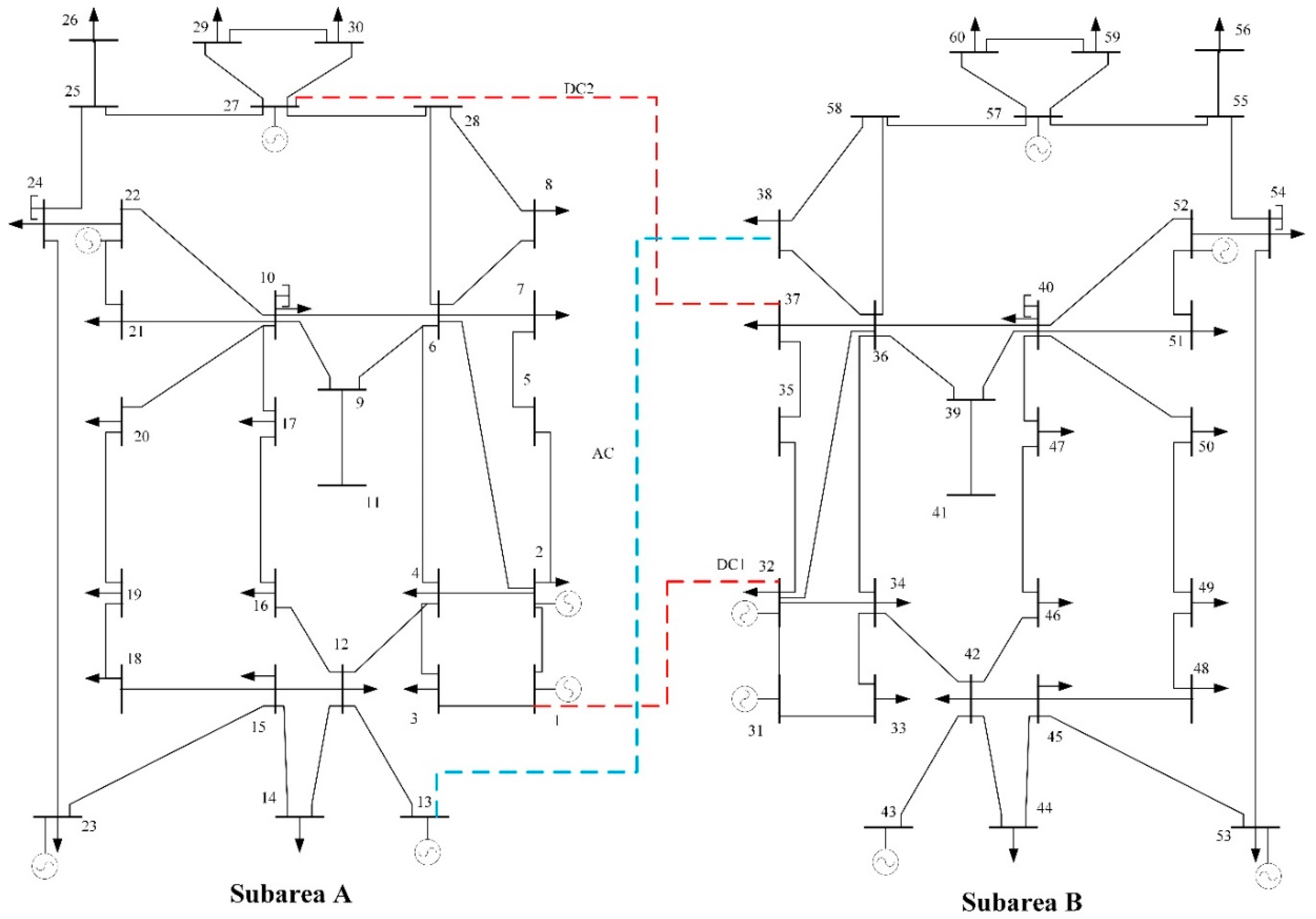
Due to AC and DC tie-lines have distinct operation modes and modeling methods, different calculation principles of net loss are adopted respectively. The net loss of the AC tie-line is proportional to the second power of its transmitted power, and the loss coefficient is related to the voltage and resistance. The net loss of the DC tie-line is proportional to its transmitted power, and the loss coefficient is related to its connection mode. The transmitted power of the DC tie-line is stair-like, thus its net loss is also distributed as stair-like.

5. Numerical Study

5.1. Basic Data

In this section, the numerical study is simulated on the improved IEEE 30-bus test system. There are two 30-bus systems, and each system consists of 20 load nodes and 6 power nodes, including one hydropower plant, one wind farm, and one photovoltaic plant. There are 3 cases in total: 30-bus subarea A of clean energy delivery, 30-bus subarea B of clean energy accommodation, and the 60-bus area which combines A and B. The power is transmitted between A and B via two AC tie-lines and one DC tie-line. The principle electrical schema of the system is shown in Appendix A. The installed generation capacity of the system is shown in

Table 1. The installed generation capacity in the system.

	Thermal Units	Hydropower Units	Wind Units	PV Units	Total
Subarea A/MW	205	50	25	20	300
Subarea B/MW	180	50	25	20	275

.

The maximum demand of subarea A is 144 MW, and the maximum demand of subarea B is 176 MW. The daily load curve of both system and the predicted output curve of clean energy units are shown in Figure 4. The numerical cases are coded by the MATLAB optimization toolkit Yalmip, and the optimization solver Gurobi is called to solve the model. The software was run on a PC made by GIGABYTE in Taiwan, China, with an Intel Core i9-8950HK 2.9 GHz CPU, and 32 GB RAM. The average computing time of scheduling subarea A, scheduling subarea B, and co-scheduling is 15 s, 12 s, and 50 s correspondingly.

Subarea A is a system with lower demand but higher capacity of units, conversely, subarea B is a system with higher demand but lower capacity of units. The end-users are independent with the generation units. Thus, the imbalance distribution of generation resources and load among regional systems is simulated. When the two subareas schedule independently, the demand of each system will be balanced with the power of their respective units and the fixed tie-line plan. When scheduling cooperatively, all the units in the two subareas will be scheduled together by SCUC and SCED algorithm to achieve the optimal results and the maximum accommodation of clean energy.

Subarea A and B schedule cooperatively is conducted to simulate the scheduling of regional power system. To embody the superiority of the method proposed by this paper, subarea A and B schedule independently is also conducted to make a comparison.

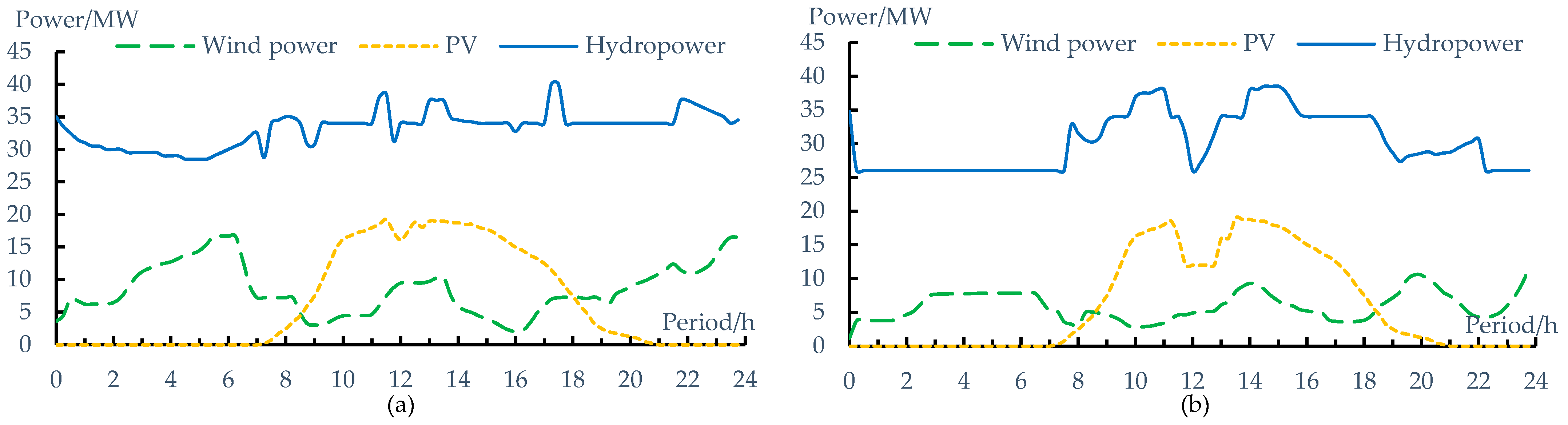
5.2. Analysis of Independent Scheduling Results

(a)

The scheduling results of subarea A

When scheduling independently, the cross-region tie-line follows the planned power curve, and the general principle is to deliver less power during the low load period and more power during the peak period. The total electricity generation cost of subarea A is $71,542. The output curves of the units are shown in Figure 5a, and the proportion of unconsumed clean energy is 7.8%.

From Figure 5a, it can be found that wind electricity abandonment mainly occurs from 19:00 to 24:00 when there is plenty of wind electricity but a reduction in load. However, both hydropower and solar power can reach an accommodation rate of more than 90%. Thus, a conclusion can be drawn that the man-made delivery plan of tie-line has a certain promotion effect on the accommodation of clean energy, but sometimes there will still be the curtailment of clean energy.

(b)

The scheduling results of subarea B

The total electricity generation cost of subarea B is $38,511. The output curves of the units are shown in Figure 5b, and the proportion of unconsumed clean energy is 14.5%.

When there is power injected into subarea B by tie-lines, the power output of the local units will be greatly affected, so the output curves will generally show a downward trend, as a result, the electricity generation cost of subarea B will be greatly reduced. It can be found from Figure 5b that hydropower curtailment is concentrated in the low period of the load “double peak”, wind power curtailment exists in various periods. Wind power and hydropower are forced to produce more than 15% of the curtailment. Therefore, it is difficult to fully consider the actual demand of the accommodation grid by the man-made delivery plan. Blindly absorbing the clean energy injected as planned will cause economic problems for the local units, even worse, this may aggravate the accommodation grid real-time scheduling pressure.

5.3. Analysis of Regional Scheduling Results

In the case of regional scheduling, the transmitted power of cross-region tie-lines is not given in advance but is obtained by optimization. When co-scheduling, the total electricity generation cost of the system was $99,855, and the proportion of unconsumed clean energy was 1.4%. The output curves of the units are shown in Figure 6a, the power transmitted by tie-line is shown in Figure 6b.

Table 2. The comparison of results in different cases.

Cases	Electricity Generation cost/th. $	Wind Power		Solar Power		Hydropower
		Electricity Generated/MWh	Accommodation Ratio	Electricity Generated/MWh	Accommodation Ratio	Electricity Generated/MWh	Accommodation Ratio
Subarea A	71.5	202.7	82.5%	155.8	98.3%	798.2	93.8%
Subarea B	38.5	141.8	80.1%	146.6	92.5%	725.6	85.3%
Area A and B	99.9	413.2	97.7%	315.2	99.5%	1906.3	98.7%

shows the comparison of the results of all the 3 cases.

When co-scheduling, the output of the units is much freer because the power transmitted between subarea A and B is no longer subject to the fixed tie-line power plan. It can be seen from Table 2 that the electricity generation cost of the united grid has been reduced by 9.2%, thus the economic benefits of the combined system have been effectively improved.

According to the method proposed by this paper, the accommodation capacity of clean energy could be further expanded through collaborative optimization and centralized scheduling. A total of 21.4% of clean energy is additionally consumed due to system combination.

As can be seen from Figure 6b, comparing with the man-made tie-line power plan, the operation of the AC and DC tie-lines optimized by the co-scheduling of the regional system is much more flexible. These tie-lines can fully release the coordination and optimization potential of the regional system, meanwhile, they play a key role in promoting the optimal allocation of generation resources and the accommodation of clean energy.

In the case of scheduling independently, subarea A sends part of the electricity to subarea B through the tie-lines, thus the power that units generated as well as the generation cost is higher in this area. At the same time, subarea B receives the power from subarea A, which reduces the generation cost. Nevertheless, this may reduce the generation activeness of the local units. Due to the power transmitted by the tie-lines is fixed, the accommodation ratio of clean energy is not ideal. Furthermore, from the point of view of the system, although subarea A and B are locally optimal, they cannot achieve global optimum.

When co-scheduling, the power transmitted by the cross-region tie-lines and the output plan of each unit are optimized by SCUC and SCED algorithm. The scheduling results of the combined system can effectively reduce the generation cost, and the clean energy can be accommodated as expected. Under the premise of satisfying the system security constraints, regional scheduling can achieve global optimum.

6. Conclusions

The regional power system can give full play to the function of generation resources optimal allocation, promoting clean energy accommodation, improving social benefits, and implementing energy policies. In this paper, the key technologies of the regional power system scheduling model—SCUC and SCED models are developed in detail. The model aims to prioritize clean energy accommodation and reduce electricity generation cost, besides, it fully considers the characteristics of the AC/DC hybrid grid network and the operation characteristics of the DC tie-line, as well as the large scale of regional system scheduling calculations. Through the verification of numerical cases, it is proved that the model and method proposed in this paper can better coordinate the power structure of the regional power system, fully explore the optimization potential of the interconnected grid, and expand the space for clean energy accommodation.

Under the trend of energy structure transformation, regional scheduling is a promising strategy, which can achieve the cleaning and high efficiency of power system. Moreover, cross-region tie-line is an essential medium to achieve regional scheduling, it indirectly determines that how much clean energy could be consumed. To improve clean energy accommodation, building more high-voltage and large capacity cross-region tie-lines is quite necessary. Accordingly, the power system should develop more flexible power sources, to supply ample peak regulation and frequency regulation capacity.

It should be pointed out that this study considers typical types of clean energy, some other types of clean energy, such as pumped-storage hydro energy [7,13], unclear energy [15], are not modeled. In further studies, the more accurate algorithm AC optimal power flow method [9] could be used in actual regional system scheduling. Meanwhile, more security constraints including cascade hydropower station constraint, gas turbine constraint could be studied.

References

1. Kaldellis, J.K.; Zafirakis, D. Prospects and challenges for clean energy in European Islands.The TILOS paradigm. Renew. Energy 2020, 145, 2489–2502. [Google Scholar] [CrossRef]
2. Mao, T.; Zhou, B.; Zhang, X.; Yao, W.; Zhu, Z. Accommodation of Clean Energy: Challenges and Practices in China Southern Region. IEEE Open J. Power Electron. 2020, 1, 198–209. [Google Scholar] [CrossRef]
3. Li, Y.; Wei, L.; Chi, Y.; Wang, Z.; Zhang, Z. Study on the key factors of regional power grid renewable energy accommodating capability. In Proceedings of the 2016 IEEE PES Asia-Pacific Power and Energy Engineering Conference (APPEEC), Xi’an, China, 25–28 October 2016. [Google Scholar]
4. Pang, R.Z.; Deng, Z.Q.; Hu, J.L. Clean energy use and total-factor efficiencies: An international comparison. Renew. Sustain. Energy Rev. 2015, 52, 1158–1171. [Google Scholar] [CrossRef]
5. Wang, Y.; Yan, W.; Zhuang, S.; Li, J. Does grid-connected clean power promote regional energy efficiency? An empirical analysis based on the upgrading grid infrastructure across China. J. Clean. Prod. 2018, 186, 736–747. [Google Scholar] [CrossRef]
6. Geng, Z.; Conejo, A.J.; Chen, Q.; Xia, Q.; Kang, C. Electricity production scheduling under uncertainty: Max social welfare vs. min emission vs. max renewable production. Appl. Energy 2017, 193, 540–549. [Google Scholar] [CrossRef] [Green Version]
7. Lin, S.; Fan, G.; Lu, Y.; Liu, M.; Li, Q. A Mixed-Integer Convex Programming Algorithm for Security-Constrained Unit Commitment of Power System with 110-kV Network and Pumped-Storage Hydro Units. Energies 2019, 12, 3646. [Google Scholar] [CrossRef] [Green Version]
8. Fu, Y.; Shahidehpour, M.; Li, Z. Security-Constrained Unit Commitment With AC Constraints. IEEE Trans. Power Syst. 2005, 20, 1001–1013. [Google Scholar] [CrossRef]
9. Nikoobakht, A.; Mardaneh, M.; Aghaei, J.; Guerrero-Mestre, V.; Contreras, J. Flexible power system operation accommodating uncertain wind power generation using transmission topology control: An improved linearised AC SCUC model. IET Gener. Transm. Distrib. 2017, 11, 142–153. [Google Scholar] [CrossRef]
10. Shi, J.; Oren, S.S. Stochastic Unit Commitment with Topology Control Recourse for Power Systems with Large-Scale Renewable Integration. IEEE Trans. Power Syst. 2017, 33, 3315–3324. [Google Scholar] [CrossRef]
11. Wu, L.; Shahidehpour, M.; Li, T. Stochastic Security-Constrained Unit Commitment. IEEE Trans. Power Syst. 2007, 22, 800–811. [Google Scholar] [CrossRef]
12. Quan, H.; Srinivasan, D.; Khosravi, A. Integration of renewable generation uncertainties into stochastic unit commitment considering reserve and risk: A comparative study. Energy 2016, 103, 735–745. [Google Scholar] [CrossRef]
13. Reck, D.; Aksel, N. Recirculation areas underneath solitary waves on gravity-driven film flows. Phys. Fluids 2015, 27, 3–28. [Google Scholar] [CrossRef]
14. Goeransson, L.; Johnsson, F. Dispatch modeling of a regional power generation system—Integrating wind power. Renew. Energy 2009, 34, 1040–1049. [Google Scholar] [CrossRef]
15. Ju, Y.; Wang, J.; Ge, F.; Lin, Y.; Dong, M.; Li, D.; Shi, K.; Zhang, H. Unit Commitment Accommodating Large Scale Green Power. Appl. Sci. 2019, 9, 1611. [Google Scholar] [CrossRef] [Green Version]
16. Lotfjou, A.; Shahidehpour, M.; Fu, Y.; Li, Z. Security-Constrained Unit Commitment With AC/DC Transmission Systems. IEEE Trans. Power Syst. 2010, 25, 531–542. [Google Scholar] [CrossRef]
17. Lotfjou, A.; Shahidehpour, M.; Fu, Y. Hourly Scheduling of DC Transmission Lines in SCUC with Voltage Source Converters. IEEE Trans. Power Deliv. 2011, 26, 650–660. [Google Scholar] [CrossRef]
18. Zhang, H.; Hu, X.; Cheng, H.; Zhang, S.; Gu, Q. Coordinated Scheduling of Generators and Tie Lines in Multi-Area Power Systems under Wind Energy Uncertainty. Energy 2021, 222, 119929. [Google Scholar] [CrossRef]
19. Barbulescu, C.; Kilyeni, S.; Vuc, G.; Lustrea, B.; Precup, R.E.; Preid, S. Software tool for power transfer distribution factors (PTDF) computing within the power systems. In Proceedings of the IEEE Eurocon, St.-Petersburg, Russia, 18–23 May 2009. [Google Scholar]
20. Denner, F.; Charogiannis, A.; Pradas, M.; Markides, C.N.; Wachem, B.G.M.V.; Kalliadasis, S. Solitary waves on falling liquid films in the inertia-dominated regime. J. Fluid Mech. 2018, 837, 491–519. [Google Scholar] [CrossRef] [Green Version]
Figure 1. The scheduling procedure of the regional power system.
Sustainability 13 02169 g001
Figure 2. The multi-segment quotation curve.
Sustainability 13 02169 g002
Figure 3. The modeling methods of AC and DC tie-line.
Sustainability 13 02169 g003
Figure 4. System load curve and predicted output curves of clean energy units.
Sustainability 13 02169 g004
Figure 5. (a) The power curves of clean energy units in subarea A; (b) The power curves of clean energy units in subarea B.
Sustainability 13 02169 g005
Figure 6. (a) The power curves of clean energy units when co-scheduling; (b) Power transmitted by tie-lines when co-scheduling.
Sustainability 13 02169 g006