Article

Decarbonizing District Heating in EU-27 + UK: How Much Excess Heat Is Available from Industrial Sites?

1
Fraunhofer Institute for Systems and Innovation Research, 76139 Karlsruhe, Germany
2
Copernicus Institute of Sustainable Development, Utrecht University, 3584 CS Utrecht, The Netherlands
3
School of Business, Innovation and Sustainability, Halmstad University, 301 18 Halmstad, Sweden
*
Author to whom correspondence should be addressed.
Sustainability 2021, 13(3), 1439; https://doi.org/10.3390/su13031439
Submission received: 22 December 2020 / Revised: 15 January 2021 / Accepted: 22 January 2021 / Published: 29 January 2021
(This article belongs to the Special Issue Heating and Cooling: Mapping and Planning of Energy Systems)

Abstract

:
Energy-intensive industries across the EU-28 release unused heat into the environment. This excess heat can be utilized for district heating systems. However, this is the exception today, and the potential contribution to the decarbonization of district heating is not well quantified. An estimation of excess heat, based on industrial processes, and spatial matching to district heating areas is necessary. We present a georeferenced industrial database with annual production and excess heat potentials at different temperature levels matched with current and possible district heating areas. Our results show a total potential of 960 PJ/a (267 TWh/a) of excess heat when the exhaust gases are cooled down to 25 °C, with 47% of the 1.608 studied industrial sites inside or within a 10 km distance of district heating areas. The calculated potentials reveal that currently 230 PJ/a (64 TWh/a) of excess heat is available for district heating areas, about 17% of today’s demand of buildings for district heating. In the future, widespread and low-temperature district heating areas increase the available excess heat to 258 PJ/a (72 TWh/a) at 55 °C or 679 PJ/a (189 TWh/a) at 25 °C. We show that industrial excess heat can substantially contribute to decarbonize district heating, however, the major share of heat will need to be supplied by renewables.

1. Introduction

Energy-intensive industrial sites (e.g., steel, cement, paper, glass, chemicals, and refineries) are spread across the member states in the European Union and UK., The production of basic materials has enormous energy needs driven by economies of scale, and mainly operate at temperatures above 1000 °C. Due to high capital cost, most of these processes are run in 3-shifts operation and only pause for maintenance needs. Thus, they often have uniform energy demands even throughout the year. Together, the energy-intensive industrial subsectors account for about 20% of the final energy consumption in EU-28 [1]. Please note, that since February 2020 there are 27 member states of The European Union, however, the geographical extent of the study is the former EU-28, which includes the United Kingdom. The largest share of the energy input is used as process heat for industrial processes like furnaces and steam generation, with 47% of process heat for high-temperature needs above 500 °C [2]. High energy costs of 3–20% of production costs [3,4] led to substantial improvements in energy efficiency in these industries in the past century. However, many industrial sites still release substantial unused energy into the environment. This excess heat from industry, sometimes also referred to as waste heat, should be further decreased as far as possible by energy efficiency measures in the individual industrial sites. Due to technical restrictions, this is only possible to a certain level. The possible use of excess heat at the same industrial site to cover the heat demand at lower temperatures is often limited [5]. Even though industrial processes need to undergo changes towards carbon-neutral fuels and process design, the high-temperature heat demands of the chemical reactions will persist. Excess heat potentials will potentially decrease due to efficiency progress in terms of energy and material use.
Excess heat from industrial sites can also be fed into a district heating (DH) system to serve as a heat source for buildings reducing the primary energy needs. DH as a way to connect unused heat from industry to buildings heat demand gained importance in the last few years like in the project Heat Roadmap Europe [6,7], or in 2016 by the EU Heating and Cooling Strategy of the Commission [8]. It is a measure towards decarbonizing the heating supply in the future, alongside with renewable-based centralized and individual heat generation where DH is not available. It is and will remain a challenge to decarbonize the mainly decentralized heating until 2050 due to the comparably low prices of fossil fuels, even with national CO2 taxes implemented, and due to various barriers to retrofitting and switching to renewables for individual building owners.
Heating demand for residential and service buildings including sanitary hot water in the EU-28 accounts for 12,344 PJ (3429 TWh) in 2018, with 64% directly based on fossil fuels [9]. Similarly, the sources for the current energy supply of district heating systems are mainly heat from cogeneration in fossil power plants, direct use of fossil fuels and municipal waste, and a small share of renewables (~5%) [10]. District heating supplied 1315 PJ (11%) in the EU-28 in 2018 to the heating of residential and service buildings, adding up to a total of 1980 PJ with industry’s heat consumption [1]. It is estimated that only about 25 PJ of industrial excess heat is recovered in European district heating systems [11]. That corresponds to a share of 2% industrial excess heat in DH for buildings.
An important pillar in the future for decarbonized heating supply is the extension of heating grids for DH and transforming them into low-temperature heating networks with typical temperatures of 30–70 °C. Low-temperature grids are described with the term 4th generation DH [12,13,14]. The low temperatures allow the inclusion of renewable sources, together with central and decentral heat pumps that increase the temperature to end-user needs. Excess heat can help transform district heating systems by providing CO2-neutral heat in large quantities in the medium term and often at comparably low costs [15]. Although in Scandinavian countries DH was ramped up in the last decades with a market share of over 50% in Sweden and Denmark for the heating supply of buildings [1,9,16], its future potential in the EU-28 is largely uncertain. Some energy system studies do not consider industrial excess heat at all [17,18], while others see an enormous potential [6,19]. A quantification of the potentials requires an analysis of the heating demand and available future heat sources like excess heat together with existing and possible future DH infrastructure with a high spatial resolution.
The estimation of industrial excess heat potentials and its utilization in district heating systems for an extended geographical context covering one or more countries is an emerging research area and the previously proposed methodologies in studies are limited. Only some approaches identify the geolocation of available excess heat. The study by Miró et al. [20] in 2015 reviewed published excess heat estimations and considered ~15% as unreliable, as temperature and system boundaries were missing. A comprehensive overview of the possible classification of methodologies was given by Brückner [21] in 2014: the scale of the study, the method of acquisition of the data (survey or estimation), and the approach (top-down or bottom-up). All of the methodologies presented here are estimations of excess heat from exhaust gases, and most of them are bottom-up, based on the calculation of the fuel input per subsector, process, or sites. One difference is the basis on which the fuel input and excess heat is calculated: emissions, national statistics per sector, or exergy analyses for each process. An overview of the presented approaches is given in Table 1. Sophisticated site-specific approaches were introduced by the study of BCS [22] for the U.S. Department of Energy in 2008 and by McKenna and Norman [23] in 2010. The latter approach was further developed by Hammond and Norman [24] in 2014. The methodologies are similar in that they estimate excess heat potentials by comparing the input energy of a process to the energy that is released at the exhaust and estimating the maximum amount of recoverable heat from this exhaust gas. The composition of the exhaust gas is derived from the input fuels and the total enthalpy of the exhaust gas based on this composition is calculated. The fuel input is estimated by production volumes per process. McKenna and Norman [23] used additionally the CO2 emissions from the European Union Transaction Log (EUTL) for the Emissions Trading System (EU ETS) data [25] and literature values to allocate the energy demand for non-energy intensive industries. A site-specific approach based on fuel input was also used in a study for the project Hotmaps [19] by Manz et al. [26], based on georeferenced annual production from various data sources multiplied by specific energy consumption values (SECs) and taking into account process-specific excess heat recovery potentials from literature. The resulting industrial excess heat was mapped with buildings’ demand by Aydemir et al. [27] by network analysis to find 170 PJ from 338 PJ excess heat could be delivered at low costs. Another process-based method presented by studies from Bühler et al. [28,29,30] used emission data per process together with energy and exergy analysis. They determine the annual excess heat potential for 80% of industrial energy demand in Denmark based on several available data sources. The energy analysis was based on the fuel, heat, and electricity demand of industrial processes. The study considered conservative estimates from literature for the fraction of input energy which is released at the exhaust and assume that 50% of this energy is recoverable. The input energy was then calculated at site level from the amount of CO2-emissions using EUTL data [25]. Brückner et al. [31] used emission reports to the federal states of Germany, that list volume flow rate and temperatures of the exhaust gases allowing a direct estimation of the excess heat which is contained in the exhaust gas streams. In Persson et al. [7] the excess heat estimation was based on subsector-specific values and greenhouse gas (GHG) emission from the European Pollutant Release and Transfer Register (E-PRTR) [32]. Svensson et al. [33] proposed to differentiate unavoidable and avoidable excess heat and calculate an excess heat temperature signature, which relies on site-specific data about the process, age, and technologies. The approaches based on processes and subsector-specific fuel demand are very data-intensive, but enable a very detailed assessment of site-specific characteristics, fuel demand, and efficiencies together with high-resolution spatial analyses for the integration of industrial excess heat into district heating systems.
Excess heat potentials can be quantified as either a theoretical, a technical (accounting for technical constraints) or an economical potential (including cost analysis). Additionally, there is also a realistic potential taking into account the barriers for utilization of excess heat. The definition of the term excess heat includes latent and sensible heat that is released by a system. The heat is transmitted either by a medium like a flue gas, a solid stream (e.g., hot coke, rolled steel, hot clinker), a liquid stream (e.g., wastewater in paper production), cooling water, or by radiation heat losses (e.g., furnace openings), or conduction heat losses (e.g., heat lost from equipment surfaces) [34,35]. A particularly large source of excess heat are the flue gases resulting from the combustion of fuels in furnaces and boilers. Flue gases, also commonly called exhaust or stack gases, are the combustion gases that emanate from industrial furnaces, ovens, boilers, and steam generators that are conveyed into the atmosphere. They contain the reaction products of the combusted fuel and air and residual substances such as sulfur oxides and particulate matter [44]. In this study, excess heat sources from energy-intensive industrial locations released via flue gases are quantified and the inclusion in district heating systems is estimated. Further excess heat potentials beyond the heat losses from flue gases are not included.
We propose a comprehensive assessment of georeferenced excess heat potentials available in the EU-28, analyzing the total potential of excess heat from the energy-intensive industries and assessing the suitability for its use in district heating grids. The quantification is based on current process design, taking into account efficiency progress. However, process change is not considered, e.g., higher share of secondary steel, switch to electrified furnaces and chemical processes based on hydrogen instead of naphtha as feedstock. The quantification is based on the assessment of current yearly energy demands by industry and buildings, therefore neglecting possible mismatch of heat loads. Furthermore, the current heat demand of buildings is used as an indicator of possible future district heating areas. The mapping of district heating areas is based on distance analysis, not on economic parameters. The main contribution of this paper is the introduction of a process-specific approach to estimating excess heat and the mapping of the results with district heating areas. The following research questions are addressed and answered:
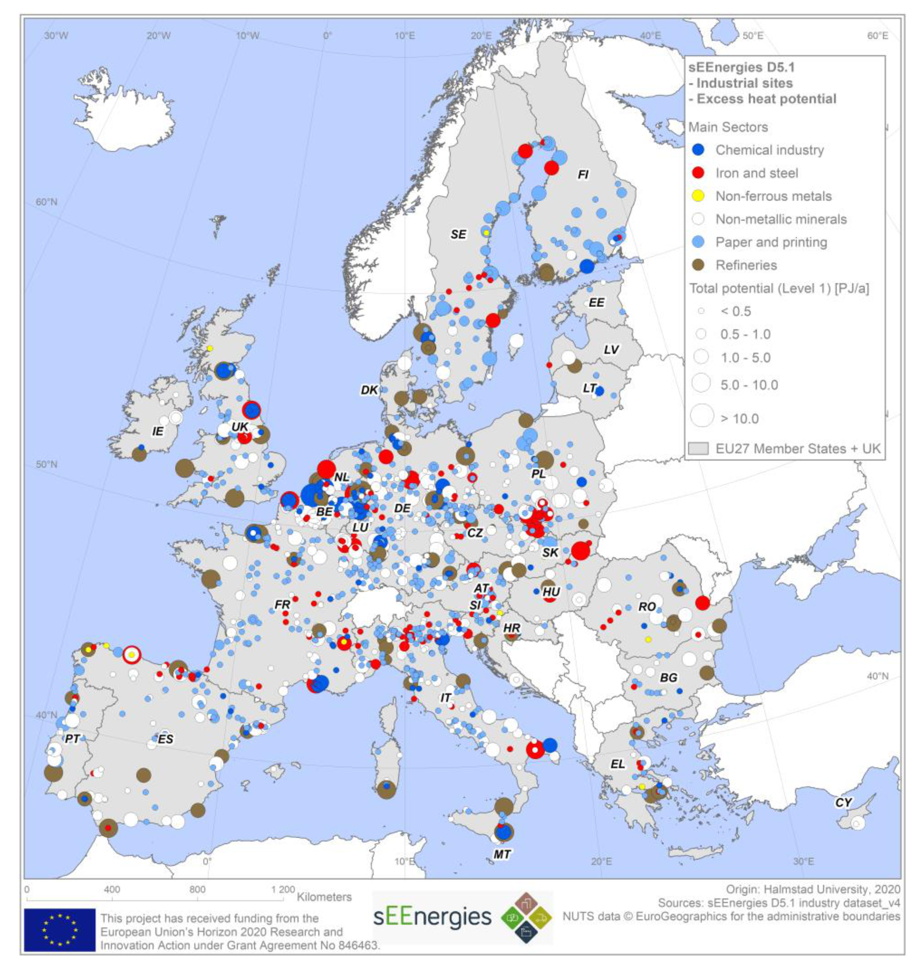
  • Where are potential sources for industrial excess heat located in the EU?
  • How much excess heat from energy-intensive industrial processes is technically available for external use?
  • How much excess heat is available for actual and possible DH systems considering efficiency measures in the industrial sector and district heating?
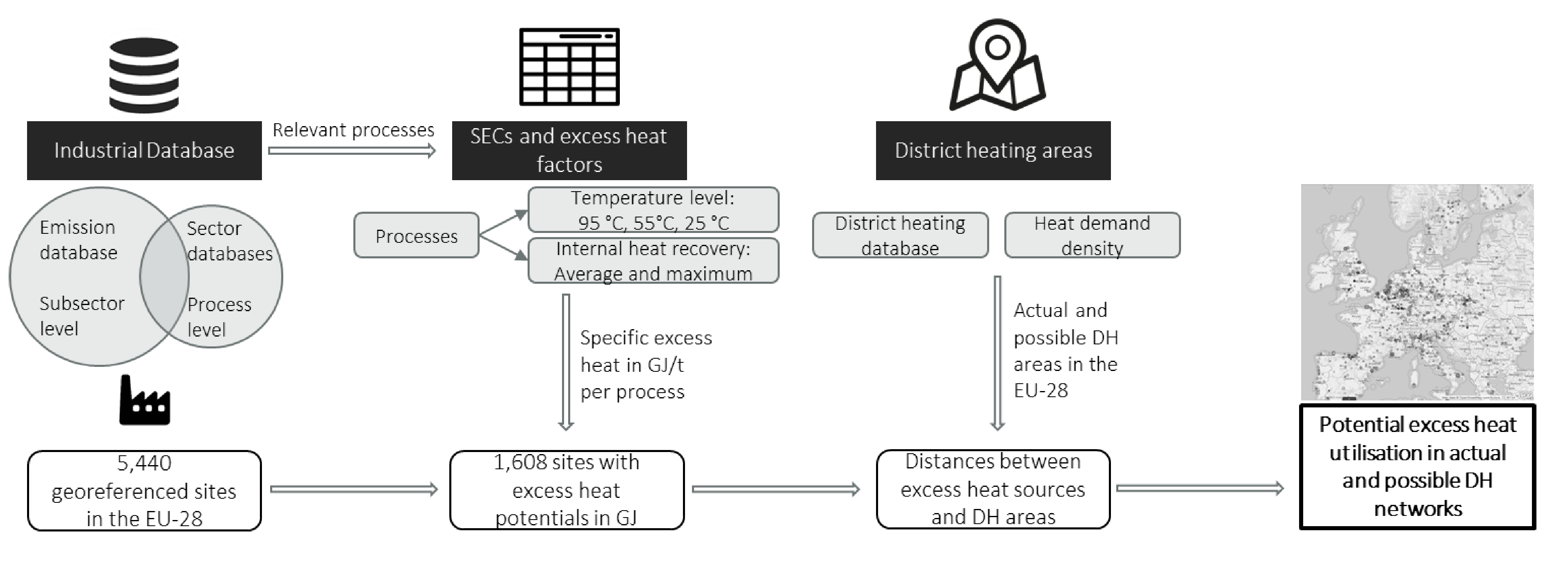
These research questions are answered with an elaborated methodology and based on extensive datasets, including georeferenced industrial sites and DH areas. The excess heat estimations are conducted at a process level. The energy demand of the processes included in this study sums up to 6891 PJ (1914 TWh) in the base year. Obtaining information about the industrial sites at the process level necessitates the collection and consolidation of several industrial datasets. Furthermore, specific energy consumption (SEC) and excess heat factors were calculated for relevant processes. The spatial mapping is conducted in a geographical information system (GIS) combining the datasets from different sources in high resolution. It enables a precise calculation of distances and the identification of the potential contribution of industrial excess heat to district heating areas. The heat sources are matched with heat demand density data and today’s DH areas. Furthermore, we analyze the excess heat potentials together with possible DH areas based on a GIS analysis of heat demand densities for all EU-28 countries.
The results presented in this paper are available as an open data set in spreadsheet and shapefiles format from the sEEnergies Open Data Hub [45], are visualized in an online Web-App [46] and are documented in the corresponding report within the EU project sEEnergies [47]. In the sEEnergies project, the presented excess heat potentials with different efficiency measures are integrated in a system analysis and spatial mapping.

2. Data and Methods

In the following subsections, the successive steps for considering the georeferenced location of heat sources (industrial sites) and heat sinks (existing and potential future district heating areas) are presented, each with the respective data and method. The analysis consists of three major steps, which are depicted in Figure 1:
  • Allocating industrial processes in the EU-28: We first map geographical locations of energy-intensive industrial sites with relevant processes and annual production in Section 2.1.
  • Estimation of process-specific excess heat potentials: We estimate specific energy consumption and excess heat on process level regardless of the geographical context in Section 2.2. The estimation depends on exhaust gas temperatures.
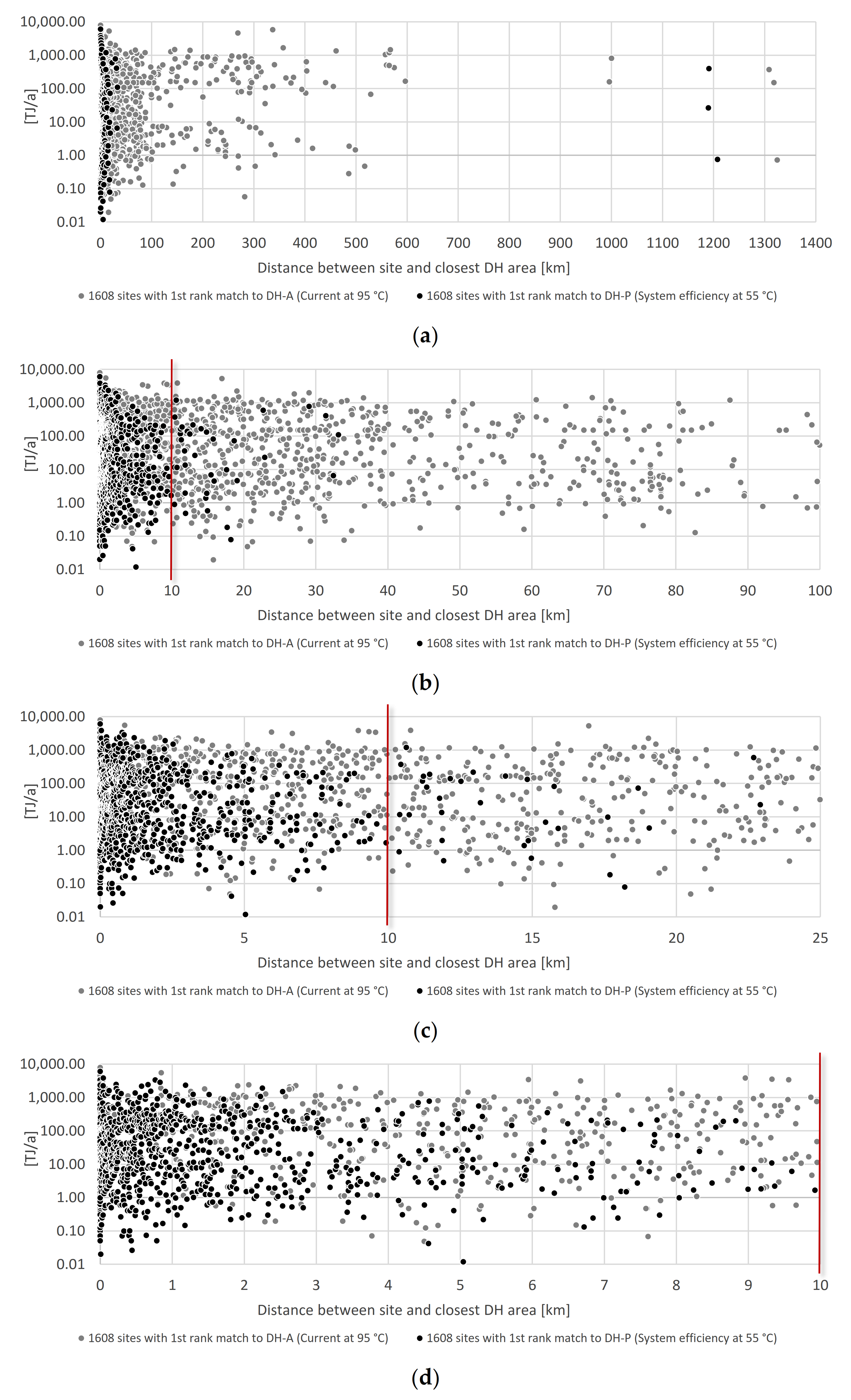
  • Mapping industrial excess heat to district heating areas: The excess heat potentials are matched with actual and possible DH systems by applying spatial GIS analyses in Section 2.3. We calculate six different potentials representing the amount of excess heat that can be supplied to district heating areas depending on the assumptions.
The availability of excess heat for DH depends on how much excess heat from the flue gases can be used internally on the same site, e.g., for preheating materials, and the temperature needs of actual and possible district heating areas. We thereby assess variations in three parameters for this analysis.
The first distinction is based on the level of internal heat recovery:
  • Current situation: many industrial processes already utilize excess heat recovery systems. The calculated excess heat potentials represent the excess heat potential available for external use for current average internal use of excess heat. This is estimated individually for each process considered.
  • Full internal use of excess heat: we assume a 100% diffusion of main internal excess heat recovery systems (e.g., for preheating materials), thereby reducing the remaining available excess heat for external use. This potential is more future-oriented and assumes that internal excess heat use is always preferable over external heat use.
The second distinction is based on the maximum heat recoverable from exhaust gases when they are cooled down to the following reference temperatures:
  • 95 °C: to estimate the maximum excess heat attainable if an exhaust gas is cooled to 95 °C. This can potentially be used directly in typical 3rd generation DH grids, which corresponds to many of the common district heating systems in operation in the EU-28.
  • 55 °C: to estimate the maximum excess heat attainable if an exhaust gas is cooled to 55 °C. This is a typical temperature for 4th generation DH grids, which will possibly be operating in the future.
  • 25 °C: to estimate the maximum excess heat attainable if an exhaust gas is cooled to ambient temperatures. This can potentially be used as a heat source for large scale heat pumps feeding into 4th generation DH grids. This value is to be considered as a maximum potential for future heating systems, even though it is quite unlikely that all of the systems can utilize these temperatures.
The last distinction is regarding the DH diffusion, i.e., grid expansion:
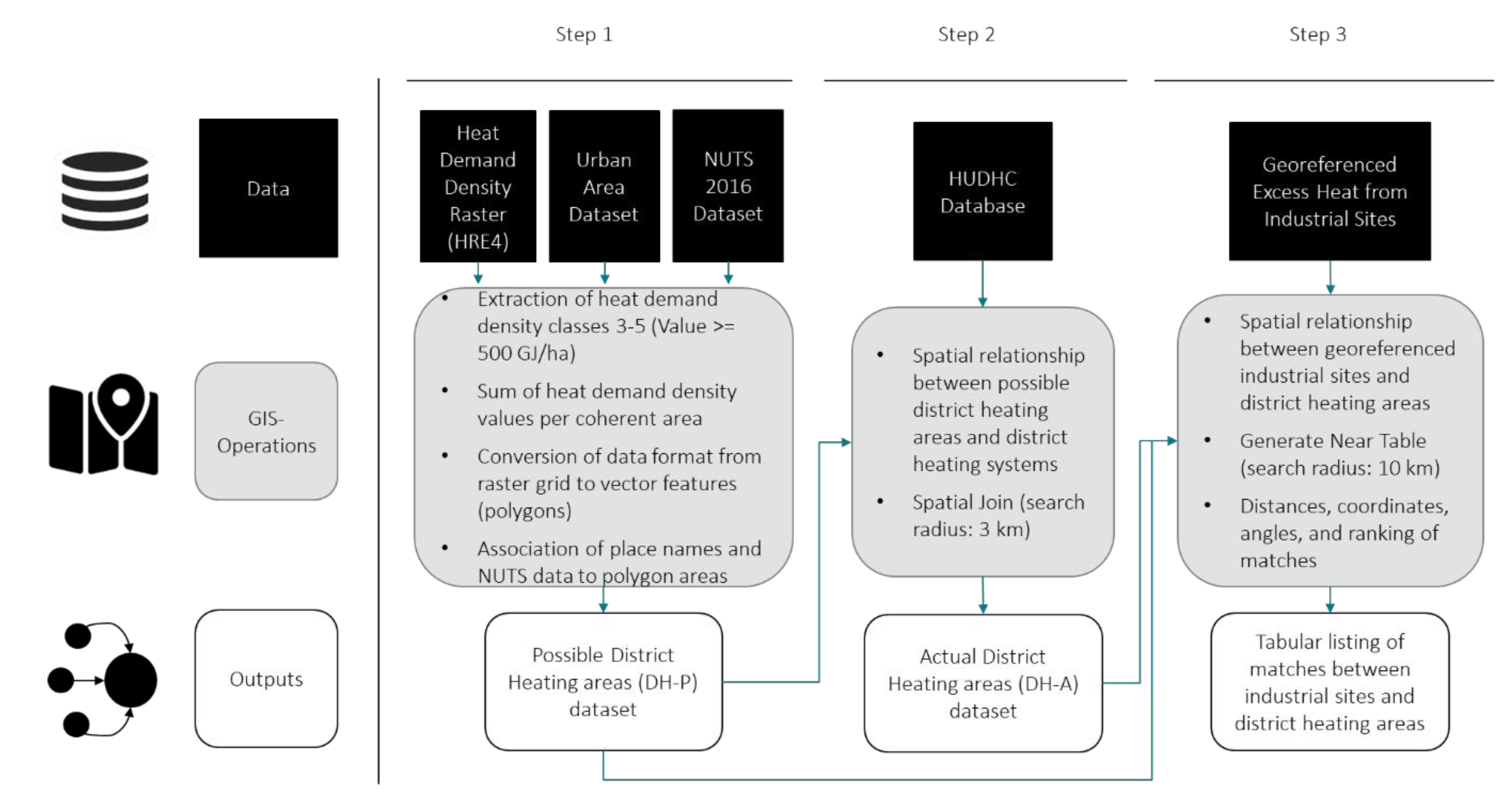
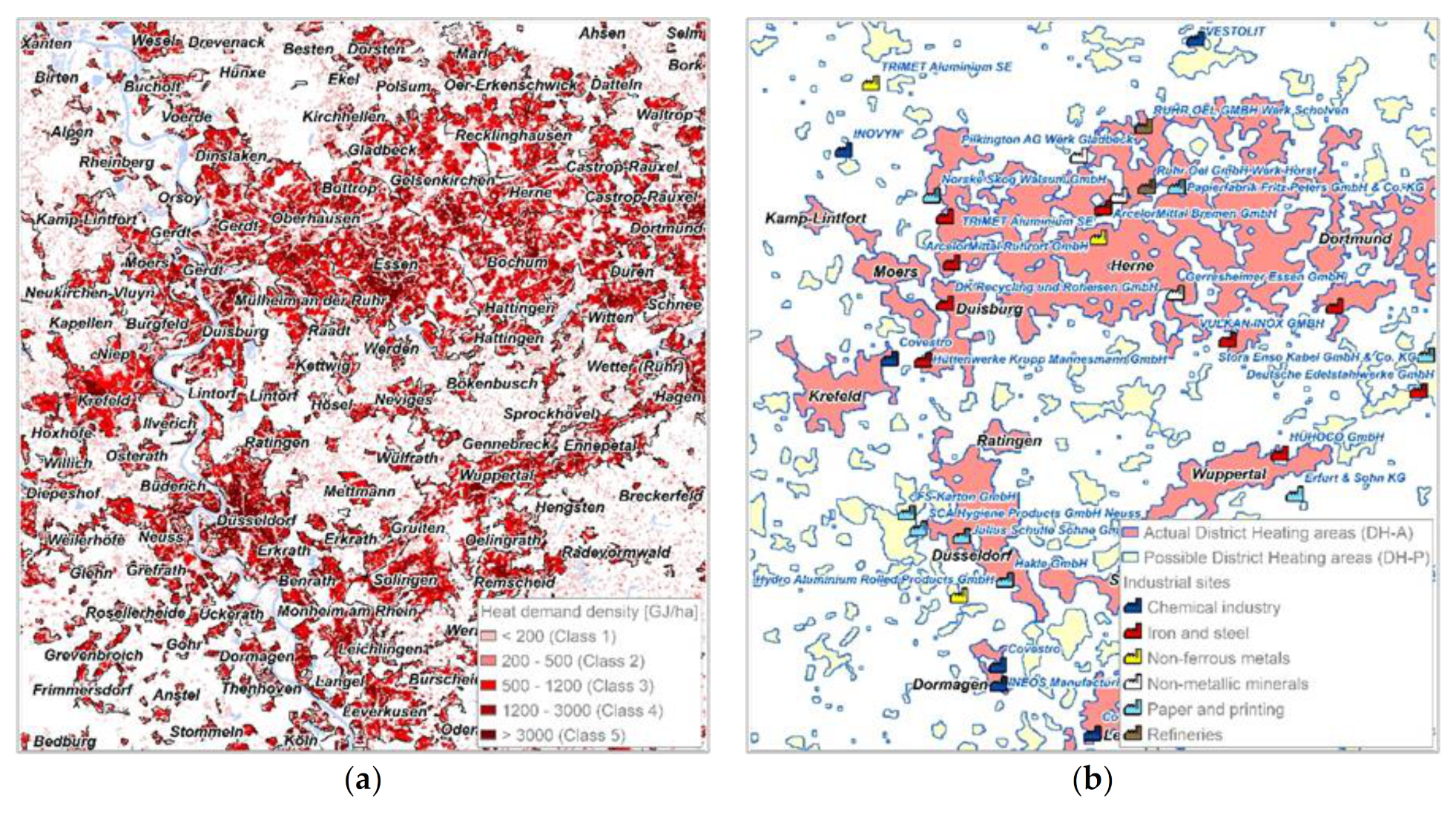
  • Actual level (DH-A): this represents the DH areas which are currently in operation in the EU-28.
  • Possible level (DH-P): this represents the potential extension of DH grids based on today’s heating demand density of buildings. These areas can currently have district heating systems already (DH-A). Areas with a current heating demand greater than 500 GJ/ha are assumed to be cost-effective or likely suitable for DH distribution. In this study, the sum of heat demands in all DH-P areas aggregates to a share of ~65% of the total heating demand by the residential and service sector in EU-28. Thus, it represents a very ambitious estimate for the possible DH areas. The reduction of useful energy demand of buildings due to renovation is not considered in the assumptions for the extension of DH systems (DH-P) (Please note, that in a previous publication [47] this potential was denominated as "expected" level).
In total, we use six different potentials to account for efficiency measures that could be implemented in industrial processes and DH systems. Table 2 summarizes the excess heat potential combinations based on the distinctions on the level of internal heat recovery and the DH system diffusion. The status quo is represented by the label Current potential. This potential includes the excess heat for the current average level of internal heat recovery in industrial sites with the exhaust gas cooled down to 95 °C and matched with current district heating areas in EU-28. The term Industrial efficiency describes potential with internal heat recovery measures that are applied to the full extent possible. However, process change to low-carbon processes or increased material efficiency are not considered. DH efficiency considers the transformation of DH to 4th generation systems, without internal efficiency improvements in industry. The maximum excess heat when exhaust gases are cooled down to 55 °C or 25 °C with spatial matching to possible DH areas is analyzed. System efficiency takes into account efficiency measures in industrial processes as full internal heat recovery in industry, and transformation to 4th generation district heating systems and is matched with a possible level of DH diffusion.

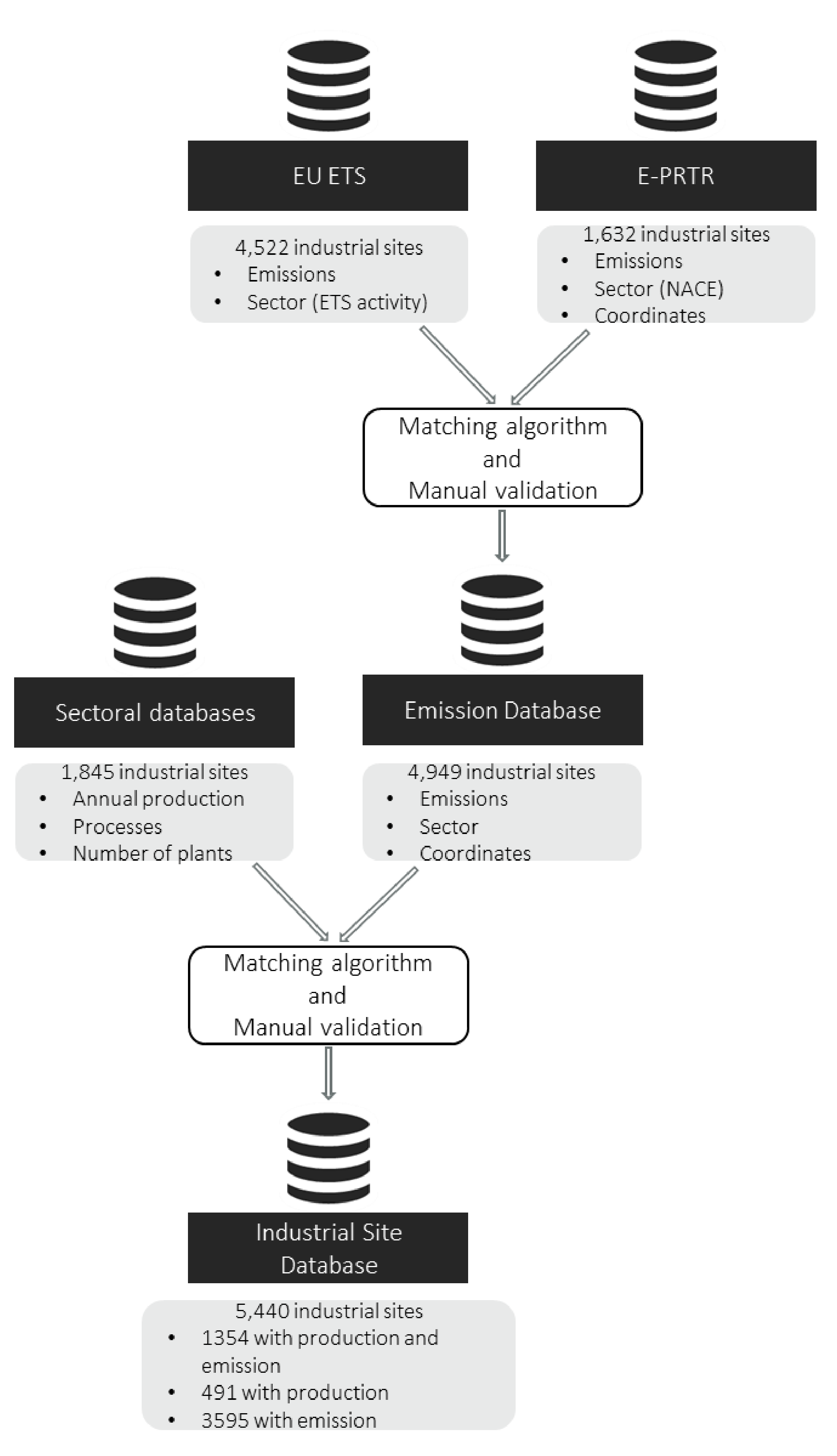
2.1. Allocating Industrial Processes in the EU-28

The objective is to construct a comprehensive database of industrial installations with the geographical area of the EU-28 including information about the annual production per process. The industrial sites are georeferenced by coordinates. A key characteristic of the Industrial Database is the inclusion of detailed information concerning the production processes and annual production of each industrial site. Thus, each data entry of an industrial production site contains the name of the company and site, the geographical location, the industrial sector, annual emission values as well as process-specific data of each associated installation such as manufactured goods and corresponding production process, annual production or production capacity. The Industrial Database covers the basic material industry producing iron and steel, non-ferrous metals (aluminum), non-metallic materials (cement, glass), chemicals (ethylene, chlorine, and ammonia), pulp and paper, and, from the energy and transformation sector, refineries. The industrial subsectors account for about 62% of the total industrial energy demand [1], therefore the database covers the main and largest industrial energy consumers in the EU-28 together with refineries, having high excess heat regarding the temperature and quantity of heat.
For the estimation of georeferenced excess heat potentials from industrial processes the following data are required:
  • coordinates or at least the address of the site;
  • industrial subsector together with production processes, or in some cases sufficient information on the manufactured goods;
  • annual production data or at least production capacity.
As no publicly available database of industrial sites includes all the information needed for process-specific allocation of production data, a new dataset based on a combination of several different datasets is created. The Industrial Database is established as a SQL database, which lists the sites as the main table. One important feature of this database is the separate tables of sites and installations. The installations relate to production process and respective annual production.
Generally, there are two types of industrial datasets: emission reporting covering the whole industrial sector and asset datasets covering single industrial subsectors. The input emission datasets are the European Pollutant Release and Transfer Register (E-PRTR) [32] and the European Union Emissions Trading System (EU ETS) from the EU Transaction Log (EUTL) [25]. The E-PRTR database contains pollutants including GHG emissions for industrial sites and other sources that emit pollutants to air, water, and land above an indicated threshold value in the EU. Most important for our analysis, it contains the coordinates of the listed sites. The industrial activities are classified by four-digit NACE codes (Statistical classification system in the EU: Nomenclature statistique des activités économiques dans la Communauté Européenne). Its objective is to establish uniform and publicly accessible national pollutant release and transfer registers in all Member States of the European Union. The EU ETS is one of the main measures introduced by the EU to achieve cost-efficient reductions of greenhouse gas emissions and reach its targets under the Kyoto Protocol and other commitments. It covers about 45% of the total emissions of CO2 equivalents in the EU by including major emission sources like power plants, aviation, and most industrial sectors. The dataset indicates only addresses of the company headquarters and defines the industrial subsectors by 40 different activities that represent the produced products. Both emission datasets were combined by matching on-site level. If one entry is listed in both datasets, the information is consolidated in one entry. The remaining entries from each dataset that are not listed in the respective other dataset are appended. The emission data of the EUTL is used if a site is listed in both datasets. Only 20% of the entries of industrial activities in EUTL can be matched with E-PRTR entries, as the threshold values for emissions to be recorded in the emission database differ. However, the matched CO2 equivalent emission values represent over 70% of all industrial EUTL emissions, because entries with high emissions are likely to be represented in both databases. In EUTL, all CO2 equivalent emissions for each industrial installation of the covered industrial sector are counted (opt-out exceptions for small installations need to be applied for); in E-PRTR threshold values for each pollutant (e.g., 100 kt CO2 per year) as well as for production for some NACE activities exist. That justifies the high number of unmatched EUTL entries.
The sectoral asset datasets used for this study originate from various, mostly commercial datasets published by a corresponding subsector association, see Table 3. These datasets are matched to the Emission Database to establish a single dataset that comprises all information available about the listed industrial sites together with all associated processes within one site, which is denominated here as an industrial installation. The methodology of the matching process is described in detail in Manz et al. [26] and depicted in Figure 2. The final database consists of 5440 industrial sites in the EU-28, listing information about 4173 installations with 37 different processes for the year 2015, of which 29 processes are identified to have excess heat potentials (for a list of the considered processes, please refer to Section 3.1.). Of these sites, 1644 are matched with both a sectoral database and at least one entry from the Emission Database. Thus, these entries include emissions on a site level and production processes on an installation level. Often, several processes (up to 13) are located at one industrial site. 491 sites from the sectoral databases cannot be matched to entries in the emission database so no GHG emissions are allocated to them. Vice versa, there are 3595 sites from the emission databases left, mainly of the production of lime, ammonia, hydrogen, bulk chemicals, and ceramics, for which no information about the production processes is retrieved from the considered sectoral databases. The matched sites of the sectoral asset databases represent a share of 27% of total sites from the Emission Database; however, they allocate a share of 64% of the industrial GHG emissions listed in EUTL, showing that the major industrial sites are included.
Often the information in the industrial database is sourced from three different input datasets: the EUTL, E-PRTR, and the respective sectoral dataset. This leads to difficulties but can also help to fill data gaps. The definition of processes and products differ: EUTL uses one of thirty defined ETS activities mainly focusing on products, while E-PRTR includes the 4-digit NACE code, which is in some cases not congruent or overlapping with the ETS activities and vice versa. Both input datasets in general contain no information about the production processes of the indicated product. The different product and process definitions can lead to the situation, that e.g., the emissions of one steel site are not totally consistent with the production capacity for steel making, sintering and coking installation, or vice versa. Another issue was addresses and coordinates in the input datasets often being wrong or slightly off from the actual location. Manual crosschecking of matched sites together with internet research is necessary. Entries from input sites that had no match with the E-PRTR do not include the coordinates. When the complete address was known, an automated look-up tool could often gain the coordinates, but otherwise checking with the company’s website was unavoidable. Furthermore, another issue is that company names change due to mergers and acquisitions, which are not updated in all datasets.

2.2. Estimation of Process-Specific Excess Heat Potentials

The methodology for quantifying the specific energy demand and the derived excess heat potentials for the processes found in the industrial database is presented in this section. To calculate the unrecovered heat from flue gases in the different industries, we adopt the bottom-up approach based on exergy applied by BCS [22]. The energy lost to exhaust gases Eex is a function of the exhaust gas mass mex and its enthalpy h. The enthalpy is dependent on the exhaust gas chemical composition and temperature T of the gases:
E e x = m e x × h = m e x × ( x i h i ) ,
where xi is the mass fraction of each component in the exhaust and hi its enthalpy. By assuming that all gases (except H2O) are ideal gases, the enthalpy of each gas component can be calculated based on the specific heat capacity of each component (Cp,i) and temperature T:
h i = T r T e x C p , i   d T ,
where Tr is the reference temperature and Tex is the temperature of the exhaust gas (for a list of the assumed exhaust temperatures please refer to Appendix A).
The enthalpy is not an absolute term and needs to be calculated against a reference state (e.g., room temperature). In this analysis, we calculate the enthalpy of exhaust gas streams at three reference temperatures of 95 °C, 55 °C, and 25 °C, to capture the heat requirements in current and future district heating systems.
In current industrial practices, exhaust gases are typically not cooled below 149 °C in order to avoid condensation of waste streams [22]. In addition, other temperature restrictions, particular to a specific exhaust stream, might apply. For example, in the case of the highly corrosive exhaust gases of glass furnaces, the gases can be cooled to a minimum temperature of 265 °C as at lower temperatures they condensate. In this analysis, we note such restrictions for every stream but do not take them into account for the calculation of excess heat.
The fraction of the excess heat lost in the exhaust (Eex) and the energy input (Ein) is equal to:
E e x E i n = m e x × x i h i m f u e l × h c ,
where, mfuel is the fuel mass and hc is the heating value of the fuel used. In this analysis, we use the lower heating value (LHV). The mass fraction of each component in the exhaust xi, and the mex/mfuel ratio are determined from combustion equations assuming full combustion and an air to fuel ratio of 10:1. For a higher air to fuel ratio, the exhaust mass flow rate to the fuel mass flow rate mex/mfuel increases, thereby increasing the estimated excess heat losses.
With the ratio of Eex/Ein the excess heat per tonne of a specific industrial product mProduct can be calculated:
E e x m P r o d u c t = E i n m P r o d u c t × E e x E i n = E i n m P r o d u c t × m e x × x i h i m f u e l × h c ,
The enthalpy of each of the exhaust gas components is calculated from the specific heat capacities (see Equation (2)). Because water vapor does not follow ideal gas behavior at low pressures, the enthalpy change was taken from steam tables for the corresponding partial pressure (by assuming atmospheric pressure, the partial pressure of water vapour is equal to the molar fraction of water in the exhaust gas mixture).
Excess heat potentials can be calculated for entries in the industrial database that include information about production processes and annual production. The production capacity is multiplied with typical sectoral utilization rates, obtaining the annual production per year mProduct,year in t/a. This is needed for the calculation of the annual excess heat potential:
E e x , y e a r = E e x m P r o d u c t × m P r o d u c t ,   y e a r ,
where Eex/mProduct is the specific excess energy per tonne of product (heat in the exhaust). It depends on the temperature of the exhaust of the specific industrial process, the level of internal heat recovery (impact on exhaust gas temperature), the temperature of the exhaust gas is cooled down, and the exhaust gas composition. The total excess heat Eex,year for each of the processes and industrial installation results from multiplication of the production in tonnes mProduct,year for the industrial process (with or without internal heat recovery) with Eex/mProduct, and is added to the Industrial Database.
In the following paragraphs, the main excess heat flue gas sources are briefly described for each industrial sector. Table 4 summarizes the temperature ranges of main gas streams and the assumptions on the composition of the fuels used or of the generated gases (when the gas composition cannot be calculated from the complete combustion of fuels). For the detailed sectoral analysis and the diffusion rates of process and recovery technologies currently employed in each industrial subsector please refer to Fleiter et al. [47].

2.2.1. Iron and Steel

Coke ovens have two sources of sensible excess heat contained: (i) in the coke oven gas (COG) and (ii) in the off-gases generated from burning COG [22]. The COG exits the coke oven at a high temperature (650 and 1000 °C). Technologies for excess heat recovery from the highly contaminated COG are available but due to the high capital costs, they are not widely implemented. The sensible heat from the off-gases is commonly recovered with a regenerator and used to preheat the incoming combustion air. The flue gases leave the regenerator at about 200 °C.
Sensible heat in blast furnaces can be recovered from two gas streams: (i) the generated blast furnace gas (BFG) and (ii) the blast stove exhaust. The gases display low temperatures; 200 °C for BFG and 250 °C for the blast stove exhaust. Heat recovery from the off-gases is a common practice [22].
The gases from basic oxygen furnaces (BOF) are very hot, with temperatures typically ranging between 1600 and 1800 °C [48]. An efficient way to utilize both the excess heat and the fuel is the non-combustion heat recovery process [49]. The BOF gas temperature in this case is reduced to about 250 °C [50].
The off-gases from electric arc furnaces (EAFs) are at high temperatures ranging from 1400–1900 °C. Scrap preheating reduces the off-gas temperature to about 200 °C. About 20% of the furnace energy input is lost as excess heat, of which in turn 50% is lost in the form of sensible heat [22].

2.2.2. Cement

Dry kilns with no heat recovery have an exhaust temperature of about 450 °C. When four preheater stages are used the temperature is lowered to 300–400 °C [51] and when the stages are increased to five or six the temperature decreases to 200–300 °C [22]. If raw material drying is not needed, the medium-low temperature heat in the kiln-off could be used for electricity generation or for supplying hot water [51].

2.2.3. Glass

Recuperative furnaces for glass production are in general the least energy-efficient furnaces used with exhaust temperatures at 980 °C. In regenerative furnaces, heat is recovered to heat the combustion air dropping the exhaust gas temperature to about 320–540 °C. Oxy-fuel smelters have exhausts with temperatures of about 1400 °C [22]. Batch/cullet preheating can lower the temperature of the flue to about 200 °C. To avoid material agglomeration, the temperature of the flue gases that enter the batch heat exchanger cannot be higher than 550–600 °C [52]. If not possible to utilize on-site, excess heat from the cooling of the flue could be potentially available for district heating. This potential could however disappear with the use of advanced batch preheaters that allow higher temperatures. Cullet preheating is currently limited in the container glass industry [52].

2.2.4. Pulp and Paper

Boilers are the largest fuel consumers generating steam for pulping, evaporation, paper making, and other operations. Exhaust temperatures from industrial boilers vary, but typical temperatures are around 260 °C with no heat recovery and 150-200 °C with heat recovery. Lime kilns, used in chemical pulping, are further important fuel consumers. The temperature of the kiln exhaust is lowered under 200 °C when heat exchangers are used [53], as cited in [54].

2.2.5. Primary Aluminum

The off-gases from aluminum smelting are responsible for only a small part of total heat losses with the most significant part stemming from the electrolytic cell surface. However, in this analysis, we only focus on the exhaust gases. The average off-gas temperature is around 700 °C [22].

2.2.6. Chemicals and Refineries

The chemical industry is quite complex with many different products generated and many small furnaces in operation for which information is scarce. We have thereby mainly focused on boiler flue gases for the industries for which information on fuel use for steam generation is available.
The hot flue gases (760–870 °C) from ethylene furnaces are typically recovered to produce steam, decreasing the flue gas temperature to about 150 °C [55]. In naphtha cracking most of the fuel consumed, about 2/3, is used in the ethylene furnace, while the remaining 1/3 is used in the separation and compression processes usually in the form of steam [56].
In ammonia production, about 40% of the fuel used for energy purposes is for steam generation [57]. In chlorine production, both for the membrane separation and the diaphragm processes the biggest part of fuel use is also for steam generation [58]. Here we assume that 100% of fuel consumption in chlorine production is by boilers. In addition, about 52% of the fuel used in refineries is consumed in boilers [57]. Exhaust temperatures from boiler flue gases are about 260 °C with no heat recovery and 150 °C (natural gas fuel) and 177 °C (refinery fuel gas) with heat recovery.

2.3. Mapping Industrial Excess Heat to District Heating Areas

The objective of this section is to describe the approach and data used to establish the spatial relationship between georeferenced industrial sites and district heating areas on an annual basis. The total annual excess heat potentials identified within the Industrial Database were matched with utilization possibilities by actual and possible DH areas. This step reduces the total external excess heat potential as only industrial locations that are located nearby a DH area represent exploitable excess heat sources. The underlying data, which was used to determine the geographical locations and areas of currently operational district heating systems in EU-28, was gathered from external data sources. Firstly, and most importantly, information on DH locations, names, and annual heat sales was gathered from the Halmstad University District Heating and Cooling database (HUDHC) [7,59,60,61]. Secondly, heat demand density raster data at hectare level was gathered for residential and service sectors of the EU Member States from the Heat Roadmap Europe project [6,60,62].
A stepwise approach consisting of three main steps was elaborated in this context, as outlined in Figure 3. Step one, the extraction of appropriate heat demand density data and converting this raster data into vector features (possible district heating areas (DH-P)), step two, relating this dataset to the HUDHC database to establish currently operational systems (actual district heating areas (DH-A), and step three, performing spatial analysis of industrial sites and district heating areas (distance calculations).
In the Heat Roadmap Europe project, heat demand densities were divided into six distinct classes with respect to the corresponding concentration of heat demands. For this study, all heat demand density grid cells with values of 500 GJ/ha and above are considered, corresponding to moderate (next to city center suburbs and multi-family building residential districts), dense, and very dense (inner urban areas) populated areas. In addition, it was found for these heating densities of the residential and service sector that economic suitability for DH distribution should be prevalent or generally likely [6]. The selected coherent areas of heating densities form the data extract with which representative areas for possible district heating areas (DH-P) can be outlined (Figure 4).
In the HUDHC database, the locations of district heating systems are given only by geographical coordinates of each corresponding city center (point sources) and hence not as spatially extended areas. This is a limitation since district heating grids are spatially distributed and spread out according to their pipe network designs. To allow a spatial analysis based on distance calculations between the georeferenced industrial sites and district heating areas, this work, therefore, includes a transformation of these point-source locations to representative district heating areas. It relies on the assumption of a likely expansion of actual DH grids operating in areas with sufficiently high heat demand densities, and the extraction of heat demand density data from the Heat Roadmap Europe dataset as indicative of such areas. The underlying evidence for this assumption consists of published results from several previous studies regarding physical and economic suitability for district heating in Europe [6,64].
The final step consisted of calculating Euclidean distances and recording matches between the industrial sites and the possible district heating areas, for which purpose the ArcGIS Proximity tool “Generate Near Table” was used within the context of a spatial model (Model Builder). The distances are measured from one industrial site to the border (spatially closest line segment) of the respective DH area. This GIS operation produces an output table with all identified matches specified by distance (in meters), coordinates, angles, and by rank (inside = 0, next closest = 1, then 2, 3, etc.). The spatial model was run iteratively for a set of different search radii (e.g. 100 km, 25 km, and 10 km) that reflect plausible transition pipe lengths for excess heat recoveries [65]. Their feasibility depends mainly on the capacities and the magnitudes of available excess heat and corresponding heat costs. The shortest and perhaps most realistic distance by which to arrange external excess heat recoveries today, 10 km, was selected to present the potentials and study results.

3. Results

In total, 1608 sites including 2567 associated installations with excess heat potentials in EU-28 were identified with the methodology presented. That means about 30% of the 5440 entries in the Industrial Database include processes analyzed for excess heat recovery in this study. The geographical locations are depicted in Figure 5, indicating the total excess heat potential of 25 °C. Sites of the non-metallic mineral subsector and paper subsector are scattered overall EU-28, having only smaller excess heat potentials. Refineries are mostly located close to the seaside or harbors, having rather high excess heat potentials. Most of the excess heat of the iron and steel production sites and from the chemical subsector is located only in a few countries, like Germany, Sweden, UK, Poland, and France.

3.1. Excess Heat Potentials per Process

The specific values of excess heat potentials per process based on the physical production are shown in Table 5. The scope of this analysis contains the flue gas streams from the 29 energy-intensive industrial processes in the database to capture the most significant high-quality excess heat sources.
Generally, the highest potential is the DH efficiency (25 °C), because it represents the potential with an average internal heat recovery of the industrial processes and the energy that could be used if the exhaust gases are cooled down to 25 °C. The difference to the Current potential is only the decrease of the temperature from 95 °C to 25 °C. Industrial efficiency and System efficiency both take into account the effects of a full internal heat recovery of excess heat, with an exhaust gas temperature of 95 °C, 55 °C, and 25 °C, respectively. The values are therefore lower than the ones with the same temperature but with today’s level of internal heat recovery. The significance of this decline varies according to the process. In the sector of non-metallic minerals, the potential for internal heat recovery is the highest and thus decreases the potential for external use significantly. For example, in the recuperative furnaces used in the container glass industry, the excess heat available is estimated at 1.8 GJ/tonne in the Current potential for the reference temperatures of 95 °C. When batch/cullet preheating is used within all plants in EU-28 (Industrial efficiency), the excess heat availability is significantly reduced to 0.2 GJ/tonne. Cooling the exhaust gas to 25 °C increases the available excess heat up to 2.6 GJ/tonne, considering preheating of the current level (40% of furnaces). The excess heat available from cooling the gases from 200 °C to 25 °C with preheating implemented in all furnaces is estimated at 0.9 GJ/tonne (System efficiency (25 °C)). The total sectoral excess heat potentials are shown in Table 6. The values represent the total available excess heat by the identified industrial processes, without consideration of DH areas. The total potentials sum up to the range of 191 to 960 PJ (53 to 267 TWh) per year in the EU-28 for the 1608 sites that have identified excess heat potentials. Most of the sites (47%) are in the pulp and paper subsector, while relatively numerous, they contribute a much smaller share to the total excess heat (~ 1%). This is because paper production sites are generally smaller both in capacity and specific energy consumption compared to the processes from the energy-intensive industries analyzed in the study. The highest potential of a single subsector is identified within the refineries, having a share of excess heat potentials of 18 up to 43%, depending on assumptions, with only 6% of the number of sites. The non-ferrous metals subsector is based solely on the primary aluminum process in this study, having a lower production compared to the other products like steel and cement. The non-metallic mineral subsector includes glass and cement clinker manufacturing, leading to a high number of sites across the EU-28 with high annual production.

3.2. Excess Heat Potential per District Heating Areas

The EU-28 residential and service sector building heat demands including hot water were assessed at about 10,800 PJ (3000 TWh) for the year 2015 by the Heat Roadmap Europe 4 project [6]. The extraction of areas with a heat density greater than 500 GJ/ha resulted in a total of 47,275 unique polygon areas for the EU-28, with the accumulated heat demands for density classes 3–5 to be at 78% (8410 PJ). The calculated sum of heat demands in possible district heating areas (DH-P) for this study constitute 65% (7018 PJ). The discrepancy is due mainly to outliers and single grid cells being omitted in the extraction process.
The database on current district heating systems (HUDHC_v5) counts a total of 4113 unique systems for the EU-28, which, if grouped by their respective CityIDs, correspond to a total of 3703-point source city coordinate pairs (latitude and longitude). From these, 2763 district heating CityIDs were found to have their city center coordinates located inside or within the maximum distance of 3 km from a possible district heating area (3025 unique systems). Therefore, they constitute the data sub-set of actual district heating areas (DH-A). Together, the matching systems constitute 98% of recorded statistics on annually sold heat in the HUDHC database (1203 PJ). For a remainder of 940 CityIDs, no matches were established: cities which currently have district heating, but where heat demand densities are below the extraction limit or beyond the maximum distance. After examination, it was found that most of these cities are in countries with high shares of district heating (e.g., Scandinavia, the Baltics, Austria, and the Slovak Republic).
Table 7 presents the results of spatial matching at the 10 km default distance of georeferenced industrial sites with respect to district heating areas for the six investigated potentials. For the Current potential, 230 PJ (64 TWh) of industrial excess heat could be utilized from 752 industrial sites, corresponding to a share of DH supply of 17% for residential and service buildings. At maximum rates of internal heat recovery, for Industrial efficiency, the annual external excess heat potential is reduced to 108 PJ (30 TWh). 1569 industrial sites (98% of the full count) were found to have 1st rank spatial matches with DH-P areas at the 10 km setting. The DH efficiency indicates annual external industrial excess heat recovery potential, depending on the exhaust gas temperature, in the range of 493 to 941 PJ (137 to 261 TWh) per year in the EU-28. This is only marginally lower than the total potentials of 504 to 960 PJ per year for the respective temperature. Even for the System efficiency, 258 to 679 PJ (72 to 189 TWh) per year are available for external heat recoveries at the 10 km distance setting.
The full distribution of 1st rank spatial matches between all 1608 industrial sites and all actual and possible district heating areas are depicted in Figure 6 for four distance settings: unlimited search radius, 100 km, 25 km, and 10 km. As can be seen at the unlimited setting, a few sites (located on Atlantic islands) constitute study population outliers at distances above 1000 km. It is clear that the main bulk of spatial matches occur within the 25 km distance for both actual and possible DH areas, while this tendency is less pronounced for actual DH areas as the distance decreases. At the 10 km default, 98% of all industrial sites (1569) have a 1st rank match to one of 11,389 DH-P areas, while 752 sites (47%) have a 1st rank match to one of 684 DH-A areas, as also detailed in Table A8. The total count of spatial matches at the 10 km setting amounts to 18,575 matches.
Most 1st rank spatial matches between industrial sites and possible DH areas are indeed happening inside or within only a few kilometers from these areas, as illustrated in Figure 6d. For the Current potential (analogous in terms of counts with the Industrial efficiency and thus relating to actual DH areas), a total of 206 sites are located inside (13%) such areas. In terms of annual energy magnitudes, the total Current potential amounts to 425 PJ of which 230 PJ per year (54%) is available in the direct vicinity of DH-A areas (within ten kilometers). Similarly, if focusing on the System efficiency (analogous in terms of counts with the DH efficiency), we find that 44% (702 sites) are located inside, 40% (639 sites) within two kilometers, and another 9% (149 sites) are located between two and five kilometers from the borders of these areas. Excess heat for external utilization originating from sites located inside or within only two kilometers from DH-P areas adds up to 90% (238 PJ per year) of the total System efficiency (55 °C) and to 91% (632 PJ per year) of the total System efficiency. (25 °C).

4. Discussion

This study presents a process-specific approach that estimates bottom-up excess heat for 29 processes from energy-intensive industrial subsectors with a spatial matching to actual and possible DH areas in the EU-28. The assessment of different temperatures and levels of internal heat recovery in the industrial processes enables taking into account efficiency measures in the important industrial sectors that decrease the available excess heat. Information concerning industrial locations was collected from various sources, stored, and georeferenced in the Industrial Database, enabling a systematic calculation of energy demand and excess heat based on the production process and annual production. The main sources of excess heat from exhaust gases for the production processes were identified and analyzed based on the temperature level and flue gas composition. In a subsequent step, the excess heat potentials were matched with the district heating database HUDHC and possible district heating systems based on heating densities with high resolution.

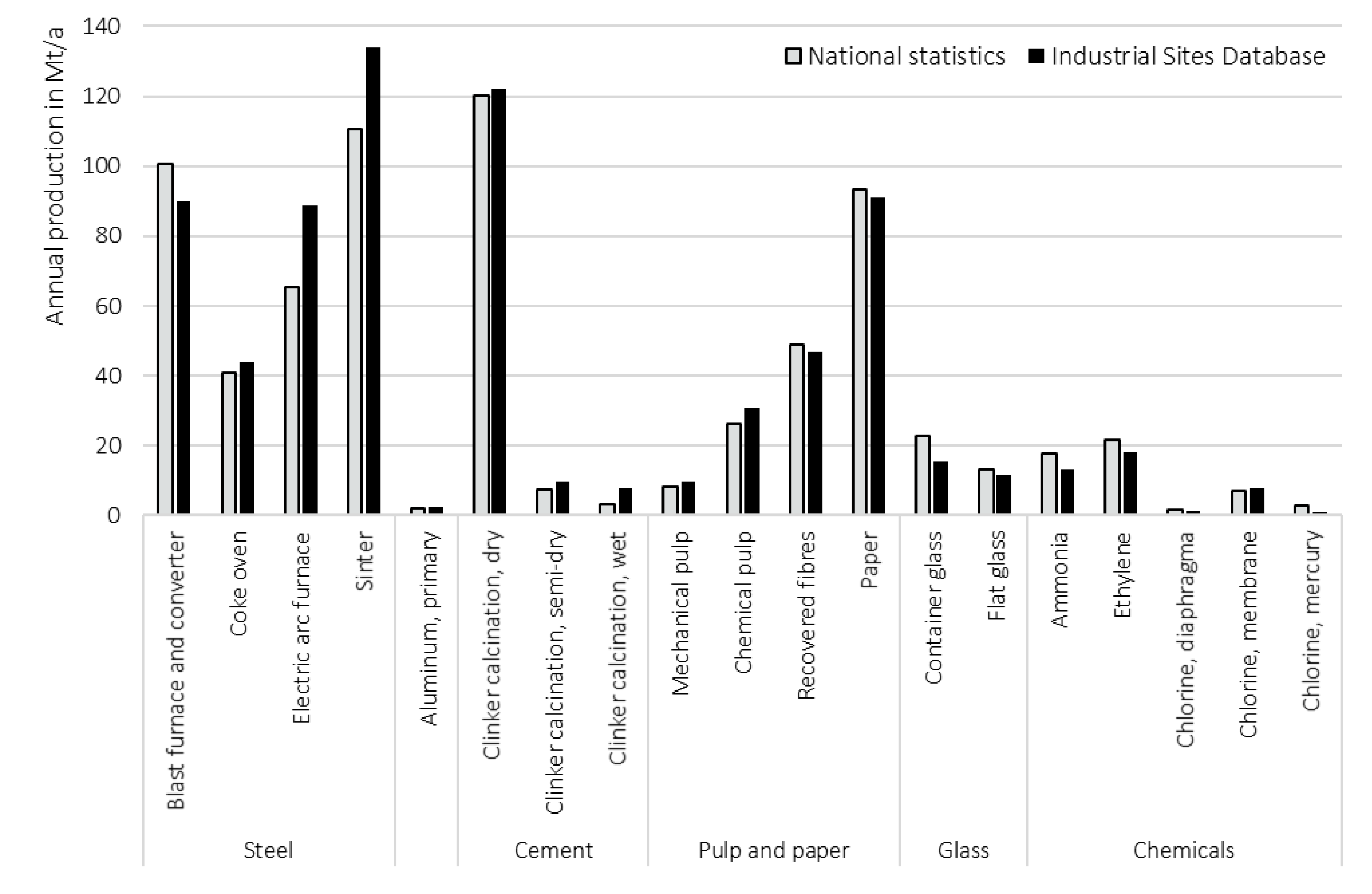
4.1. Data Validation

The excess heat potentials calculated based on physical production for each production process were benchmarked with excess heat estimations found in other studies (see Table 1). The deviations are shown in Figure 7. Please note, that for this validation the spatial analysis is omitted, and the total excess heat potentials are used. Depending on the assumptions in the other publications, the best fitting value depending on temperature and internal heat recovery was chosen for comparison. The calculation method of the literature values differs in many cases from the one presented here. Furthermore, the input data regarding the inclusion of industrial processes and the assumed temperature levels can differ greatly. Compared to Brückner et al. [34], the value for Germany is comparable with −5%. It should be noted, that for similar temperatures comparable values are found even though our approach is based on production data instead of emissions. This holds true for the values that were found for a full internal heat recovery which corresponds best to the conservative assumptions. Compared to Pehnt et al. [66], there is a deviation of +219% for Germany, originating from a different methodology. The deviation for EU-28 of +205% to Persson et al. [7] can be explained by a different methodology of excess heat calculation using average estimates per sector. This comparison can hint at the fact that sectoral values are prone to overestimate the potentials compared to a process-specific approach. The approach from Manz et al. [26] is similar to the one presented in this study, without the chemical sector and refineries. When the respective value is compared, there is a deviation of +2% remaining. Regarding the values for Denmark from the study of Bühler et al. [29], there is a deviation of +311%, as it covers most sites of the industrial sector in Denmark (80% of industrial final energy consumption). As Denmark has only a few industrial sites from the energy-intensive industry, a lot of processes are from non-energy intensive subsectors that are not included in our study. As a summary, our values are within the range of other studies presented before. With our approach, process-specific efficiency measures and even change of process can be considered in contrast to subsector-based values. It should be emphasized that our bottom-up approach for the EU-28 inherently underestimates the available potentials because it focuses on the largest point sources, major processes, and flue gases as the most attractive excess heat streams. Although the analysis covers the most attractive potentials, including additional excess heat sources would increase the potentials available, particularly at lower temperatures.
The data quality of the Industry Database regarding the annual production and annual fuel consumption is validated with EU statistics for each country and process. In Figure 8, a comparison of the production data is validated with national production data on country level. The national data is taken from sectoral associations with gaps filled with data from PRODCOM [67], as presented in [2]. It is based on the year 2015. The national values indicate that most of the processes are covered completely by the Industrial Database, but for some processes, there is a deviation up to 20%. This can have several reasons: the most important factor is a remaining uncertainty regarding annual utilization factors where only production capacity is given to calculate the annual production. When the statistical production is greater than what can be found in the database, it also indicates that some smaller installation could be missing. In general, the comparison shows that the database has a sufficient quality to estimate process-specific excess heat potentials, even though it can be refined and checked persistently.

4.2. Limitations

Even though various efficiency measures both in industry and DH are considered in this study to capture future developments, it is not a scenario-based analysis and important expectable structural changes are therefore not integrated. In general, energy-intensive processes are currently mainly based on fossil fuels and additionally often have process-related CO2 emissions. A transformation to carbon-neutral processes, such as the replacement of blast furnaces by hydrogen (direct reduction, plasma) and electricity-based (electric arc furnace) processes, and the electrification of furnaces and steam generation might lead to different excess heat potentials. Consequent circular economy and material efficiency will lead to less primary production of these energy-intensive materials. Refineries especially will face structural change until 2050, producing for example synthetic fuels. In addition, future excess heat potentials for use in DH must be evaluated under the assumption that industrial locations are likely to be situated where they are now and there is no or little shift of production to other countries outside the EU-28. Furthermore, district heating systems are expected to face a decreasing heating demand due to higher building standards and renovation of buildings. The heating demand in this study neglects the influence of a decreasing heating demand or communal initiatives promoting the installation or extension of DH, instead calculating the possible DH areas with today’s heating density where competitiveness was already proven [6].
Moreover, the data basis for all calculation steps can be improved continuously. The deviation of national production data from the georeferenced data implies that sites are missing, that the calculation of annual production from capacity among individual sites varies significantly and not all closure of sites are recorded. The inclusion of further industrial processes, cross-cutting technologies like machines, less energy-intensive, heterogeneous sectors, and even other low-temperature excess heat sources like data centers or wastewater treatment plants is limited with the methodology presented. The HUDHC database [59] lists 4113 DH systems in the EU-28, a number that captures the largest DH city systems, but probably misses some minor DH systems as nobody knows exactly how many district heating systems are currently in operation in the EU-28. However, regarding the data used, most large-size district heating systems operated over long time periods are included, while those missing mainly refer to smaller systems and more recent developments. The data displays a 68% coverage rate regarding statistics on annual heat sales, which is improvable. The possible DH areas are based on today’s heating densities by buildings that will be reduced in the future due to refurbishments and thus lowering the feasibility for DH.
For the calculation of excess heat potentials, exhaust gas temperature and quality restrictions due to condensation and corrosive materials are not taken into account. Although the heat could still be recovered at lower temperatures, it would require more advanced technologies and different materials [44,68]. We therefore emphasize the need to intensify R&D activities for technical solutions (e.g., heat exchangers for corrosive gases or filters for chemicals). Heat sources other than flue gases are neglected. This leads to a rather conservative estimate as other significant sources of excess heat such as from solid and liquid streams, cooling water, radiation, and conduction heat losses are not considered. However, the excess heat potential within the scope of this study comprises the most relevant potentials, being large major point sources and often providing heat at high-temperature levels. Thus, exploiting sources beyond our system boundary would probably involve higher specific costs, as smaller excess heat streams would need to be addressed. Still, further research should also include such excess heat sources that probably will also become more attractive with the diffusion of heat pumps and technical learning of these systems.
In this study, we quantified the possible contribution of industrial excess heat to DH areas based on annual values, which is justified due to the work being organized mostly in three shifts in energy-intensive industries. However, this neglects the fact that some industries do not produce throughout the entire year e.g., the cement industry mostly closes in the winter months due to a decreased demand in the construction sector. Higher time resolutions of the excess heat availability and the match with demand was not considered in our study. In Bühler et al. [28], it can be seen that these factors could reduce the potential by 30%.
Furthermore, the economic potential is not evaluated. As a next step, costs for pipes and DH extension could be included [6,28]. Instead, we base our assumptions on the findings of Heat Roadmap Europe [6] and on a focus on the 10 km default distance range. Our findings emphasize that the pipe length is most probably not the limiting factor. A cost analysis is needed to prioritize the measure that will be cost-efficient at a system level: applying best available technologies and efficiency measures in processes, using the excess heat internally at the site, or feeding the heat into DH systems. But it should be noted, that especially for DH networks, costs are not the only factor defining the realization of such long-term projects, the framework conditions and communal strategies are also very important.
As a summary, the limitation shows that there are uncertainties in excess heat estimations, that can be overcome or decreased with further research, but some will persist, as excess heat utilization is dependent on local parameters. In the end, there are factors that could increase the estimated potential, others could limit it further.

4.3. Conclusions

The results show that there are at least 1608 large point sources of industrial excess heat available, across different subsectors. Refineries have the largest potentials with a total excess heat potential of 331 PJ/a at status quo, allocated to only about 100 sites. The production of chemicals and steel have high average excess heat potentials per site, each with only around 100 sites in the EU-28. The sites that produce paper, cement, and glass are more distributed, having lower average excess heating potentials per site. The amount of heat that is available depends mainly on two factors: the heat recovery measures that use the excess heat internally, and the temperature at which the exhaust gas is cooled down. These factors should always be included in excess heat estimations, as we found total excess heat potentials from all 1608 industrial sites ranging from 191 to 960 PJ/a depending on the assumptions.
The excess heat currently available from industrial flue gases for use in district heating is significant: About 230 PJ can be recovered and used in current DH systems (95 °C), which corresponds to 17% of today’s DH demand of buildings for space heating and hot water. This share can be significantly higher for single DH areas and regions, where industrial sites can deliver high amounts of excess heat. Compared to the 25 PJ of industrial excess heat recovery in European district heating systems [11], a rough estimate on this basis would suggest that current industrial excess heat volumes inside or within 10 km of actual district heating areas are nine times higher. The main sources would be the energy-intensive processes in the refineries, cement kilns, and blast furnaces.
The wide implementation of heat recovery in industries limits the excess heat available for district heating: The wide adoption of main internal heat recovery can reduce the currently available excess heat potential by 53% to 108 PJ/a, which, however, is still more than four times the current external recovery level. The industrial subsectors where we assume that there is still a great potential for efficiency measures such as increasing the internal heat recovery, contribute most to the reduction of the overall potential. That is predominantly the non-metallic minerals subsector (−73%) with cement and glass manufacturing.
The utilization of excess heat at 55 °C doubles the excess heat potentials available for district heating: If DH systems are extended and all are transformed to 4th generation by reducing the operating temperature, the number of sites that are in a 10 km radius of DH areas increases from 752 to 1569 (98% of all sites), with about 83% of these within 2 km. With that, the excess potentials at 55 °C compared to the temperature of 95 °C increase from 230 to 493 PJ/a for average internal heat recovery, and from 108 to 258 PJ/a for maximum heat recovery.
The implementation of 4th generation DH networks with large scale heat pumps substantially increases the heat recovery potentials: The further reduction of exhaust gas temperature to 25 °C increases the excess heat potential at a 10 km distance up to 941 PJ/a at average rate of an internal heat recovery. If the maximum potential of efficiency measures in industrial sites is applied, this potential is reduced by 28% to 679 PJ/a. In this analysis, 25 °C are shown as a lower estimate to depict the maximum potential for the supply of 4th generation DH networks with large-scale heat pumps or of cold DH networks where the heat is supplied to the end-consumer with a heat pump (decentral or central at substations).
Industrial sites are located often within 2 km to district heating areas: Considering that 83% of all industrial sites analyzed and 91% of the total annual excess heat potential at 692 PJ (25 °C, with internal heat recovery for industry) are located inside or within 2 kilometers from possible DH areas, we expect a high economic feasibility for the connection of most industrial sites recovering excess heat in the EU-28. Combining excess heat sources and the deployment of district heating systems should therefore be a central element in the transition towards a sustainable and CO2-neutral heating and cooling sector. However, the analysis also shows that industrial excess heat alone will not be sufficient, and the major heat source for district heating will need to come from renewable energy sources.

Author Contributions

Conceptualization, P.M., K.K., Urban Persson and T.F.; Data curation, P.M., K.K., U.P., M.N. and T.F.; Formal analysis, P.M., K.K., U.P. and T.F.; Funding acquisition, U.P., T.F. and W.C.-G.; Investigation, P.M., K.K. and Urban Persson; Methodology, P.M., K.K., U.P., M.N., T.F. and W.C.-G.; Project administration, U.P., T.F. and W.C.-G.; Resources, T.F. and W.C.-G.; Supervision, T.F. and W.C.-G.; Validation, P.M., K.K., Urban Persson and T.F.; Visualization, P.M., K.K., U.P. and M.N.; Writing—original draft, P.M., K.K. and U.P.; Writing—review & editing, P.M., K.K., U.P., M.N., T.F. and W.C.-G. All authors have read and agreed to the published version of the manuscript.

Funding

This research was funded by the project sEEnergies, European Union’s Horizon 2020 Research and Innovation Action under Grant Agreement No 846463.

Data Availability Statement

The data presented in this study are openly available here: As shapefiles and spreadsheets from the sEEnergies Open Data Hub D5.1: https://s-eenergies-open-data-euf.hub.arcgis.com/. Visualized in an online Web-App: https://tinyurl.com/sEEnergies-D5-1.

Conflicts of Interest

The authors declare no conflict of interest.

Appendix A. Detailed Industry Specific Fuel Demand, Exhaust Temperatures and Excess Heat Estimates

In the following, the assumptions used for the calculation of the excess heat per process are presented per subsector. It includes the temperatures of the exhaust gas, the SEC per tonne of respective product, the calculated percentage of available excess heat of the fuel input or the absolute values in GJ/tonne of the product and the diffusion rate of processes within the sites that produce the specific product. The assumed future diffusion rate accounts for the implementation of more efficient process design in the future.
Table A1. Iron and Steel Industry. Assumptions: SEC values from [69]. For more details see [47].
Exhaust Gas Temperature (°C)Fuel SEC (GJ/t)UnitAbsolute or Relative Excess HeatCurrent Diffusion Rate (%)Assumed Future Diffusion Rate (%)
25 °C55 °C95 °C
Coke ovens
Sensible heat in COG816-GJ/tonne coke0.980.950.91100%0%
Sensible heat in COG; with HR449-GJ/tonne coke0.470.440.400%100%
Excess heat in off-gases2001.6% of fuel input44%13%9%100%100%
Blast furnaces
Sensible heat in BFG221-GJ/tonne steel0.420.360.27100%100%
Blast stove exhaust2501.5 % of fuel input13%10%8%50%0%
Blast stove exhaust; with HR1301.49% of fuel input6%4%2%50%100%
Basic oxygen furnace
Sensible heat in BOF off-gases1704-GJ/tonne steel0.560.550.5430%0%
Sensible heat in BOF off-gases; with HR250-GJ/tonne steel0.020.020.0170%100%
Electric arc furnace
Electric arc furnace12041.8% of fuel input12%12%12%70%0%
Electric arc furnace; with HR2041.5% of fuel input2%1%1%30%100%
Table A2. Non-ferrous Metals Industry. Source: [69] for electricity demand and [22] for excess heat estimation.
Exhaust Gas Temperature (°C)Electricity SEC (GJ/t)Unit% of Fuel Input as Excess HeatCurrent Diffusion Rate (%)Assumed Future Diffusion Rate (%)
25 °C55 °C95 °C
Primary aluminium70054GJ/tonne aluminium1.091.051.00100%100%
Table A3. Glass Industry: Specific values based on produced glass in tonne. Assumptions: To estimate the SECs per technology with and without batch/cullet preheating, we used the fuel use reported in [69] as an average, and we assumed that for 40% of the production it is 15% lower and for 60% of the production 15% higher. The typical energy savings from batch/cullet preheating are around 10–20% [52]. For more details see [47].
Exhaust Gas Temperature (°C)Fuel SEC (GJ/t)Unit% of Fuel Input as Excess HeatCurrent Diffusion Rate (%) ()Assumed Future Diffusion Rate (%)
25 °C55 °C95 °C
Container glass
Recuperative9826.2% of fuel input60%47%45%60%0%
Recuperative; with HR2004.6% of fuel input19%7%5%40%100%
Regenerative4275.2% of fuel input30%18%16%60%0%
Regenerative; with HR2003.8% of fuel input19%7%5%40%100%
Oxy-fuel14275.2% of fuel input35%30%29%60%0%
Oxy-fuel; with HR2003.8% of fuel input8%3%2%40%100%
Flat glass
Recuperative9829.2% of fuel input60%47%45%100%0%
Recuperative; with HR2007.8% of fuel input19%7%5%0%100%
Regenerative4277.5% of fuel input30%18%16%100%0%
Regenerative; with HR2006.4% of fuel input19%7%5%0%100%
Oxy-fuel14275.6% of fuel input35%30%29%100%0%
Oxy-fuel; with HR2004.8% of fuel input8%3%2%0%100%
Table A4. Cement Industry: Specific values based on produced clinker in tonne. Assumptions: SEC from [69]. Current diffusion rate not applicable as production volumes are known for each kiln technology. For more detail see [47].
Exhaust Gas Temperature (°C)Fuel SEC (GJ/t)Unit% of Fuel Input as Excess HeatCurrent Diffusion Rate (%)Assumed Future Diffusion Rate (%)
25 °C55 °C95 °C
Wet3385.5% of fuel input20%15%13%not needednot needed
Dry4494.5% of fuel input27%22%20%not needednot needed
Dry, with preheating and precalciner (4 stage preheating)3383.3% of fuel input22%17%15%not needednot needed
Dry with preheating and precalciner (5-6 stage preheating)2503.0% of fuel input17%12%10%not needednot needed
Table A5. Pulp and Paper Industry: Specific values based on produced pulp (pulp making) or paper (paper making) in tonne. For more details see [47].
Exhaust Gas Temperature (°C)Fuel SEC (GJ/t)Unit% of Fuel Input as Excess HeatCurrent Diffusion Rate (%)Assumed Future Diffusion Rate (%)
25 °C55 °C95 °C
Pulp making
Chemical pulping26012.3% of fuel input9%3%3%30%0%
Chemical pulping; with HR17710.3% of fuel input8%2%1%70%100%
Lime burning6502.2% of fuel input52%36%34%30%0%
Lime burning; with HR2001.4% of fuel input24%8%6%70%100%
Mechanical pulping2602.2% of fuel input9%3%3%30%0%
Mechanical pulping; with HR1771.9% of fuel input8%2%1%70%100%
Recovered fibres2600.6% of fuel input9%3%3%30%0%
Recovered fibres, with HR1770.5% of fuel input8%2%1%70%100%
Paper making
Board & packaging paper2605.7% of fuel input9%3%3%30%0%
Graphic paper2608.4% of fuel input9%3%3%30%0%
Tissue paper2608.1% of fuel input9%3%3%30%0%
Board & packaging paper; with boiler HR1774.9% of fuel input8%2%1%70%100%
Graphic paper; with boiler HR1777.2% of fuel input8%2%1%70%100%
Tissue paper; with boiler HR1776.9% of fuel input8%2%1%70%100%
Table A6. Chemical Industry: Specific values based on produced product in tonne. Assumptions: SEC estimated from the fuel use reported in [69], while also accounting for the share of production that uses boiler economizers and the share that does not. When economizers are used, 5–10% of the fuel use can be saved [70]. For more details see [47].
Exhaust Gas Temperature (°C)Fuel SEC (GJ/t)Unit% of Fuel Input as Excess HeatCurrent Diffusion Rate (%)Assumed Future Diffusion Rate (%)
25 °C55 °C95 °C
Ethylene
Furnace14923.9% of fuel input17%4%3%100%100%
Boiler26013.3% of fuel input22%10%8%30%0%
Boiler, with HR14911.4% of fuel input17%4%3%70%100%
Ammonia
Boiler2605.1% of fuel input22%10%8%30%0%
Boiler, with HR1494.4% of fuel input17%4%3%70%100%
Chlorine diaphragm
Boiler2603.6% of fuel input22%10%8%30%0%
Boiler; with HR1493.1% of fuel input17%4%3%70%100%
Chlorine membrane
Boiler2601.2% of fuel input22%10%8%30%0%
Boiler, with HR1491.0% of fuel input17%4%3%70%100%
Table A7. Refineries: Specific values based on produced product in tonne. Assumptions: SEC estimated from the fuel use reported in [69], while also accounting for the share of production that uses boiler economizers and the share that does not. When economizers are used, 5–10% of the fuel use can be saved [70]. In boilers fired with by-product fuels, such as refinery fuel gas, the minimum final exhaust temperature after waste heat recovery is more likely to be higher compared to when conventional fuels are used [22]. For more details see [47].
Exhaust Gas Temperature (°C)Fuel SEC (GJ/t)Unit% Of Fuel Input as Excess HeatCurrent Diffusion Rate (%)Assumed Future Diffusion Rate (%)
25 °C55 °C95 °C
Boiler, no HR
Refinery basic2601.60% of fuel input29%11%9%30%0%
Refinery gasoline focused2602.00% of fuel input29%11%9%30%0%
Refinery diesel focused2602.30% of fuel input29%11%9%30%0%
Refinery flexible; 2602.10% of fuel input29%11%9%30%0%
Boiler, with HR
Refinery basic1771.40% of fuel input24%6%4%70%100%
Refinery gasoline focused1771.70% of fuel input24%6%4%70%100%
Refinery diesel focused1772.00% of fuel input24%6%4%70%100%
Refinery flexible1771.80% of fuel input24%6%4%70%100%

Appendix B. Detailed Industry Specific Fuel Demand, Exhaust Temperatures and Excess Heat Estimates

Table A8. Summary table for 1st rank spatial matches with reference to the Current potential and System efficiency at 55 °C and 25 °C by distance classes.
ScenarioDimensionInside (0 km)Up to <2 km>2 up to <5 km5 up to 10 km10 up to <25 km25 up to <100 km>100 kmTotal
Current potentialMatches DH-A (n)2061871631963243831491608
Share (%)13%12%10%12%20%24%9%100%
Matches (Acc.) (n)206393556752107614591491608
Share (Acc.) (%)13%24%35%47%67%91%9%100%
Current potential (95 °C)Heat (PJ/a)54605264776653425
Share (%)13%14%12%15%18%16%12%100%
Heat (Acc.) (n)5411416623030637353425
Share (Acc.) (%)13%27%39%54%72%88%12%100%
System efficiencyMatches DH-P (n)7026391497932431608
Share (%)44%40%9%5%2%0.25%0.19%100%
Matches (Acc.) (n)7021341149015691601160531608
Share (Acc.) (%)44%83%93%98%99.6%99.8%0.2%100%
System efficiency (55 °C)Heat (PJ/a)132106174410.4264
Share (%)50%40%6%2%1%0.5%0.2%100%
Heat (Acc.) (n)1322382542582622630.4264
Share (Acc.) (%)50%90%96%98%99%99.8%0.2%100%
System efficiency (25 °C)Heat (PJ/a)3842483991021.5692
Share ()55%36%6%1%1%0%0%100%
Heat (Acc.) (n)3846326716796896912692
Share (Acc.) (%)55%91%97%98%100%100%0%100%

References

  1. Eurostat. Complete Energy Balances (Table nrg_bal_c). 2020. Available online: https://ec.europa.eu/eurostat/data/database (accessed on 15 July 2020).
  2. Rehfeldt, M.; Fleiter, T.; Toro, F. A bottom-up estimation of the heating and cooling demand in European industry. Energy Effic. 2017, 45, 786. [Google Scholar] [CrossRef]
  3. European Commission. Energy Prices and Costs in Europe; COM (2019) I Final; European Commission: Brussels, Belgium, 2019. [Google Scholar]
  4. Eichhammer, W.; Walz, R. Industrial Energy Efficiency and Competitiveness. In Development Policy, Statistics and Research Branch; Working Paper 05/2011; United Nations Industrial Development Organization: Vienna, Austria, 2011. [Google Scholar]
  5. Aydemir, A.; Rohde, C. What About Heat Integration? Quantifying Energy Saving Potentials for Germany. In ECEEE Industrial Summer Study Proceedings; European Council for an Energy-Efficient Economy—ECEEE: Berlin, Germany, 13 June 2018; pp. 197–205. [Google Scholar]
  6. Persson, U.; Wiechers, E.; Möller, B.; Werner, S. Heat roadmap Europe: Heat distribution costs. Energy 2019, 176, 604–622. [Google Scholar] [CrossRef]
  7. Persson, U.; Möller, B.; Werner, S. Heat Roadmap Europe: Identifying strategic heat synergy regions. Energy Policy 2014, 74, 663–681. [Google Scholar] [CrossRef]
  8. European Commission. An EU Strategy on Heating and Cooling. Communication from the Commission to the European Parliament, the Council, the European Economic and Social Committee and the Committee of the Regions; COM(2016) 51 Final; European Commission: Brussels, Belgium, 2016. [Google Scholar]
  9. Odyssee-Mure. Odyssee Database. 2020. Available online: www.odyssee-mure.eu (accessed on 1 September 2020).
  10. Colmenar-Santos, A.; Borge-Díez, D.; Rosales-Asensio, E. District Heating and Cooling Networks in the European Union; Springer International Publishing: Cham, Switzerland, 2017; ISBN 978-3-319-57952-8. [Google Scholar]
  11. Persson, U.; Werner, S. District heating in sequential energy supply. Appl. Energy 2012, 95, 123–131. [Google Scholar] [CrossRef]
  12. Lund, H.; Werner, S.; Wiltshire, R.; Svendsen, S.; Thorsen, J.E.; Hvelplund, F.; Mathiesen, B.V. 4th generation district heating (4GDH). Energy 2014, 68, 1–11. [Google Scholar] [CrossRef]
  13. Werner, S. International review of district heating and cooling. Energy 2017, 137, 617–631. [Google Scholar] [CrossRef]
  14. Nielsen, S.; Möller, B. GIS based analysis of future district heating potential in Denmark. Energy 2013, 57, 458–468. [Google Scholar] [CrossRef] [Green Version]
  15. Möller, B.; Wiechers, E.; Persson, U.; Grundahl, L.; Lund, R.S.; Mathiesen, B.V. Heat roadmap Europe: Towards EU-Wide, local heat supply strategies. Energy 2019, 177, 554–564. [Google Scholar] [CrossRef]
  16. Euroheat & Power. Country by Country District Heating and Cooling. 2019. Available online: https://www.euroheat.org/knowledge-hub/country-profiles/ (accessed on 1 September 2020).
  17. European Commission. EU Reference Scenario 2016: Energy, Transport and GHG Emissions—Trends to 2050; European Commission: Brussels, Belgium, 2016. [Google Scholar]
  18. International Energy Agency. World Energy Outlook 2019; IEA Publications: Paris, France, 2019; ISBN 9789264973008. [Google Scholar]
  19. Pezzutto, S.; Zambotti, S.; Croce, S.; Zambelli, P.; Garegnani, G.; Scaramuzzino, C.; Pascuas, R.P.; Haas, F.; Exner, D.; Lucchi, E.; et al. D2.3 WP2 Report—Open Data Set for the EU28: Deliverable D2.3 Hotmaps; European Commission: Brussels, Belgium, 2019. [Google Scholar]
  20. Miró, L.; Brückner, S.; Cabeza, L.F. Mapping and discussing Industrial Waste Heat (IWH) potentials for different countries. Renew. Sustain. Energy Rev. 2015, 51, 847–855. [Google Scholar] [CrossRef] [Green Version]
  21. Brückner, S.; Miró, L.; Cabeza, L.F.; Pehnt, M.; Laevemann, E. Methods to estimate the industrial waste heat potential of regions—A categorization and literature review. Renew. Sustain. Energy Rev. 2014, 38, 164–171. [Google Scholar] [CrossRef]
  22. BCS Inc. Waste Heat Recovery: Technology and Opportunities in U.S. Industry; U.S. Department of Energy, Office of Energy Efficiency and Renewable Energy, Industrial Technologies Program: Washington, DC, USA, 2008.
  23. McKenna, R.C.; Norman, J.B. Spatial modelling of industrial heat loads and recovery potentials in the UK. Energy Policy 2010, 38, 5878–5891. [Google Scholar] [CrossRef]
  24. Hammond, G.P.; Norman, J.B. Heat recovery opportunities in UK industry. Appl. Energy 2014, 116, 387–397. [Google Scholar] [CrossRef] [Green Version]
  25. European Environment Agency. European Union Emissions Trading System (EU ETS) Data from EUTL (EU Transaction Log.). 2020. Available online: https://www.eea.europa.eu/ds_resolveuid/DAT-21-en (accessed on 25 February 2020).
  26. Manz, P.; Fleiter, T.; Aydemir, A. Developing a Georeferenced Database of Energy-intensive Industry Plants for Estimation of Excess Heat Potentials. In ECEEE Industrial Summer Study Proceedings; European Council for an Energy-Efficient Economy—ECEEE: Berlin, Germany, 13 June 2018; pp. 239–247. [Google Scholar]
  27. Aydemir, A.; Fleiter, T.; Schilling, D.; Fallahnejad, M. Industrial Excess Heat and District Heating: Potentials and Costs for the EU-28 on the Basis of Network Analysis. In ECEEE Industrial Summer Study Proceedings; European Council for an Energy-Efficient Economy—ECEEE: online, 30 September 2020. [Google Scholar]
  28. Bühler, F.; Petrović, S.; Holm, F.M.; Karlsson, K.; Elmegaard, B. Spatiotemporal and economic analysis of industrial excess heat as a resource for district heating. Energy 2018, 151, 715–728. [Google Scholar] [CrossRef] [Green Version]
  29. Bühler, F.; Petrović, S.; Karlsson, K.; Elmegaard, B. Industrial excess heat for district heating in Denmark. Appl. Energy 2017, 205, 991–1001. [Google Scholar] [CrossRef] [Green Version]
  30. Bühler, F.; Nguyen, T.-V.; Elmegaard, B. Energy and exergy analyses of the Danish industry sector. Appl. Energy 2016, 184, 1447–1459. [Google Scholar] [CrossRef] [Green Version]
  31. Brückner, S. Industrielle Abwärme: Bestimmung von Gesichertem Aufkommen und Technischer bzw. Wirtschaftlicher Nutzbarkeit; TU München: München, Germany, 2016. [Google Scholar]
  32. European Environment Agency. The European Pollutant Release and Transfer Register (EPRTR), Member States Reporting under Article 7 of Regulation (EC) No 166/2006. Available online: https://www.eea.europa.eu/ds_resolveuid/DAT-26-en (accessed on 25 February 2020).
  33. Svensson, E.; Morandin, M.; Harvey, S. Characterization and visualization of industrial excess heat for different levels of on-site process heat recovery. Int. J. Energy Res. 2019, 43, 7988–8003. [Google Scholar] [CrossRef] [Green Version]
  34. Brückner, S.; Arbter, R.; Pehnt, M.; Laevemann, E. Industrial waste heat potential in Germany—A bottom-up analysis. Energy Effic. 2017, 10, 513–525. [Google Scholar] [CrossRef]
  35. Pehnt, M.; Bödeker, J.; Arens, M.; Jochem, E.; Idrissova, F. Die Nutzung Industrieller Abwärme—Technisch-Wirtschaftliche Potenziale und Energiepolitische Umsetzung: Wissenschaftliche Begleitforschung zu Übergreifenden Technischen, Ökologischen, Ökonomischen und Strategischen Aspekten des Nationalen Teils der Klimaschutzinitiative; Fraunhofer-Verlag: Berlin/Heidelberg, Germany, 2010. [Google Scholar]
  36. Energetics; E3M. Energy Use, Loss and Opportunities Analysis: U.S. Manufacturing & Mining; Prepared for the U.S. Department of Energy—Energy Efficiency and Renewable Energy Industrial Technologies Program; U.S. Department of Energy: Washington, DC, USA, 2004.
  37. Sollesnes, G.; Helgerud, H.E. Utnyttelse av Spillvarme fra Norsk Industri: En Potensialstudie; Enova Rapport 2009:1; Norsk Energi: Oslo, Norway, 2009. [Google Scholar]
  38. Papapetrou, M.; Kosmadakis, G.; Cipollina, A.; La Commare, U.; Micale, G. Industrial waste heat: Estimation of the technically available resource in the EU per industrial sector, temperature level and country. Appl. Therm. Eng. 2018, 138, 207–216. [Google Scholar] [CrossRef]
  39. European Commission. Industrial Thermal Energy Recovery Conversion and Management. D 2.1 Literature Review of Energy Use and Potential for Heat Recovery in the Eu28 Report; European Commission: Brussels, Belgium, 2016. [Google Scholar]
  40. Panayiotou, G.P.; Bianchi, G.; Georgiou, G.; Aresti, L.; Argyrou, M.; Agathokleous, R.; Tsamos, K.M.; Tassou, S.A.; Florides, G.; Kalogirou, S.; et al. Preliminary assessment of waste heat potential in major European industries. Energy Procedia 2017, 123, 335–345. [Google Scholar] [CrossRef]
  41. Forman, C.; Muritala, I.K.; Pardemann, R.; Meyer, B. Estimating the global waste heat potential. Renew. Sustain. Energy Rev. 2016, 57, 1568–1579. [Google Scholar] [CrossRef]
  42. Bianchi, G.; Panayiotou, G.P.; Aresti, L.; Kalogirou, S.A.; Florides, G.A.; Tsamos, K.; Tassou, S.A.; Christodoulides, P. Estimating the waste heat recovery in the European Union Industry. Energy Ecol. Environ. 2019, 4, 211–221. [Google Scholar] [CrossRef] [Green Version]
  43. Miró, L.; McKenna, R.; Jäger, T.; Cabeza, L.F. Estimating the industrial waste heat recovery potential based on CO2 emissions in the European non-metallic mineral industry. Energy Effic. 2018, 11, 427–443. [Google Scholar] [CrossRef] [Green Version]
  44. Aydemir, A.; Fritz, M. Estimating excess heat from exhaust gases: Why corrosion matters. Energy Ecol. Environ. 2020, 28, 1359. [Google Scholar] [CrossRef]
  45. Fleiter, T.; Manz, P.; Neuwirth, M.; Mildner, F.; Persson, U.; Kermeli, K.; Crijns-Graus, W.; Rutten, C. D5.1 Industry Dataset; sEEnergies Open Data: Flensburg, Germany, 2020. [Google Scholar]
  46. Fleiter, T.; Manz, P.; Neuwirth, M.; Mildner, F.; Persson, U.; Kermeli, K.; Crijns-Graus, W.; Rutten, C. sEEnergies D5.1 Dataset Web-App; ArcGIS Online; Europa-Universität Flensburg: Flensburg, Germany, 2020. [Google Scholar]
  47. Fleiter, T.; Manz, P.; Neuwirth, M.; Mildner, F.; Persson, U.; Kermeli, K.; Crijns-Graus, W.; Rutten, C. Documentation on Excess Heat Potentials of Industrial Sites Including Open Data File with Selected Potentials; (Revised Version); ZENODO: Geneva, Switzerland, 2021. [Google Scholar]
  48. International Energy Agency. Tracking Industrial Energy Efficiency and CO2 Emissions Energy Indicators; International Energy Agency: Paris, France, 2007. [Google Scholar]
  49. European Commission. Best Available Techniques (BAT) Reference Document for Iron and Steel Production. Industrial Emissions Directive 2010/75/EU (Integrated Pollution Prevention and Control); Publications Office of the European Union: Luxembourg, 2013; ISBN 9789279264764. [Google Scholar]
  50. Ray, H.S.; Singh, B.P.; Bhattacharjee, S.; Misra, V.N. Energy in Minerals and Metallurgical Industries; Allied Publishers: New Delhi, India, 2005; ISBN 8177648748. [Google Scholar]
  51. European Commission. Best Available Techniques (BAT) Reference Document for the Production of Cement, Lime and Magnesium Oxide. Industrial Emissions Directive 2010/75/EU (Integrated Pollution Prevention and Control); Publications Office of the European Union: Luxembourg, 2013; ISBN 978-92-79-32944-9. [Google Scholar]
  52. European Commission. Best Available Techniques (BAT) Reference Document for the Manufacture of Glass. Industrial Emissions Directive 2010/75/EU (Integrated Pollution Prevention and Control); Publications Office of the European Union: Luxembourg, 2013; ISBN 978-92-79-28284-3. [Google Scholar]
  53. Hough, G. (Ed.) Chemical Recovery in the Alkaline Pulping Processes; TAPPI Pr: Atlanta, GA, USA, 1985; ISBN 0898520460. [Google Scholar]
  54. Lundqvist, P. Mass and Energy Balances Over the Lime Kiln in a Kraft Pulp Mill. Master’s Thesis, Uppsala University, Uppsala, Sweden, 2009. [Google Scholar]
  55. Hendricks, T.; Choate, W.T. Engineering Scoping Study of Thermoelectric Generator Systems for Industrial Waste Heat Recovery; US DOE Office of Energy Efficiency and Renewable Energy (EERE): Washington, DC, USA, 2006.
  56. Boulamanti, A.; Moya, R.J.A. Energy Efficiency and GHG Emissions: Prospective Scenarios for the Chemical and Petrochemical Industry; EUR—Scientific and Technical Research Reports; Publications Office of the European Union: Brussels, Belgium, 2017. [Google Scholar] [CrossRef]
  57. United States Department of Energy. Steam System Opportunity Assessment for the Pulp and Paper, Chemical Manufacturing, and Petroleum Refining Industries: Main Report; United States Department of Energy: Washington, DC, USA, 2002.
  58. Jörissen, J.; Turek, T.; Weber, R. Chlorherstellung mit Sauerstoffverzehrkathoden. Energieeinsparung bei der Elektrolyse. Chem. Unserer Zeit 2011, 45, 172–183. [Google Scholar] [CrossRef]
  59. Halmstad University. Halmstad University District Heating and Cooling Database_Version 5; (2016 Update by Date 2019-09-30); Halmstad University: Halmstad, Sweden, 2019. [Google Scholar]
  60. Persson, U.; Möller, B.; Wiechers, E. Methodologies and Assumptions Used in the Mapping. In Heat Roadmap Europe 2050, A Low-Carbon Heating and Cooling Strategy; European Commission: Brussels, Belgium, 2017. [Google Scholar]
  61. Persson, U.; Averfalk, H. Accessible Urban Waste Heat: Deliverable D1.4 ReUseHeat. In Recovery of Urban Excess Heat; European Commission: Brussels, Belgium, 2018. [Google Scholar]
  62. Europa-Universität Flensburg. Pan-European Thermal Atlas 4.3 (PETA 4.3). In Heat Roadmap Europe—A Low-Carbon Heating and Cooling Strategy for Europe; European Commission: Brussels, Belgium, 2018. [Google Scholar]
  63. Wiechers, E.; Möller, B.; Persson, U. D5.2 Urban Area Dataset; sEEnergies Open Data: Flensburg, Germany, 2020. [Google Scholar]
  64. Persson, U.; Werner, S. Heat distribution and the future competitiveness of district heating. Appl. Energy 2011, 88, 568–576. [Google Scholar] [CrossRef]
  65. Kavvadias, K.C.; Quoilin, S. Exploiting waste heat potential by long distance heat transmission: Design considerations and techno-economic assessment. Appl. Energy 2018, 216, 452–465. [Google Scholar] [CrossRef]
  66. Pehnt, M.; Arens, M.; Jochem, E.; Bödeker, J.; Idrissova, F. Industrial Waste Heat-Tapping into a Neglected Efficiency Potential. In ECEEE Dummer Study Proceedings; European Council for an Energy-Efficient Economy—ECEEE: Munich, Germany, 2011. [Google Scholar]
  67. Eurostat. Statistics on the Production of Manufactured Goods. Total Production by PRODCOM List (NACE Rev. 2)—Annual Data (DS-066342). Available online: https://ec.europa.eu/eurostat/web/prodcom/data/database (accessed on 15 July 2020).
  68. Brough, D.; Jouhara, H. The aluminium industry: A review on state-of-the-art technologies, environmental impacts and possibilities for waste heat recovery. Int. J. Thermofluids 2020, 1–2, 10007. [Google Scholar] [CrossRef]
  69. Fleiter, T.; Elsland, R.; Herbst, A.; Manz, P.; Popovski, E.; Rehfeldt, M.; Reiter, U.; Catenazzi, G.; Jakob, M.; Harmsen, R.; et al. Baseline Scenario of the Heating and Cooling Demand in Buildings and Industry in the 14 MSs Until 2050: Heat Roadmap Europe Deliverable D3.3 and D3.4; European Commission: Brussels, Belgium, 2017. [Google Scholar]
  70. Kermeli, K.; Worrel, E.; Graus, W.; Corsten, M. Energy Efficiency and Cost Saving Opportunities for Ammonia and Nitrogenous Fertilizer Production; United States Environmental Protection Agency: Washington, DC, USA, 2017.
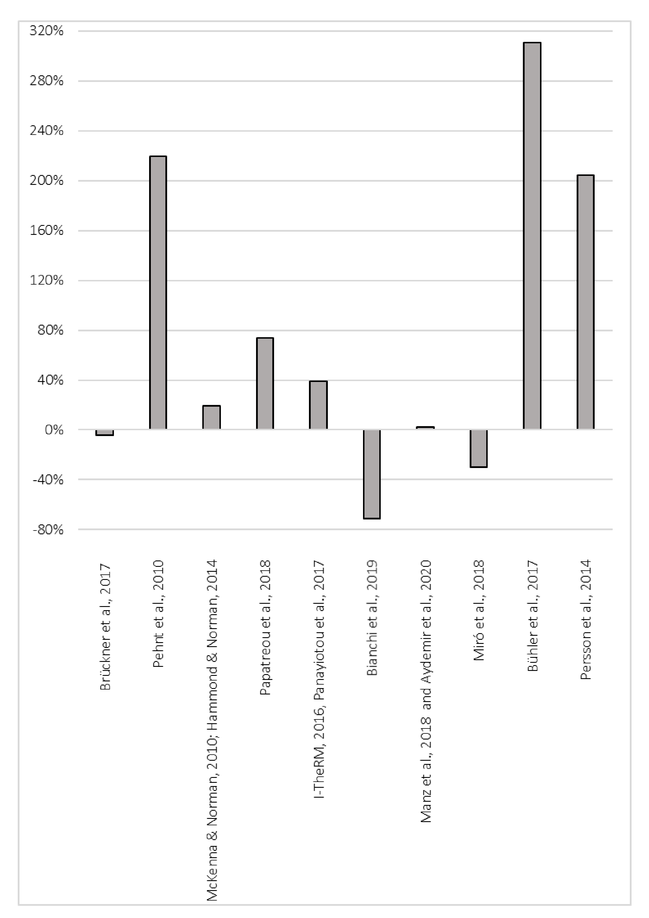
Figure 1. Schematic calculation steps in this analysis.
Sustainability 13 01439 g001
Figure 2. Establishing the Industrial Database for the member states of The European Union and the UK EU-28.
Sustainability 13 01439 g002
Figure 3. Principal overview of the three main steps used in the spatial mapping of industrial sites and district heating areas. Source for Urban Area Dataset: [63].
Sustainability 13 01439 g003
Figure 4. Heat demand density classification by hectare grid cells for residential and service sector building heat demands (a) and the spatial relationship between georeferenced industrial sites to possible district heating areas (DH-P) and actual district heating areas (DH-A) (b), exemplified for Düsseldorf and surroundings in Germany.
Sustainability 13 01439 g004
Figure 5. Total excess heat potential (25 °C, average internal heat recovery) of the 1608 georeferenced industrial sites by sectors in the EU-28.
Sustainability 13 01439 g005
Figure 6. Distribution of 1st rank spatial matches between industrial sites and district heating areas by distance for Current potential (relative DH-A, grey dots) and System Efficiency (55 °C) (relative DH-P, black dots), with annual excess heat volumes per site in TJ/a for all distances (a), within 100 km (b), within 25 km (c), and within the study default 10 km limit (d).
Sustainability 13 01439 g006
Figure 7. Deviations of excess heat potentials found in this study.
Sustainability 13 01439 g007
Figure 8. Production per process as stated in statistics of sectoral associations on national level (label: National) and included in industrial database (label: Process specific). Data source: [2].
Sustainability 13 01439 g008
Table 1. Comparison of excess heat estimations in literature.
StudyMethodCommentsTemperature Level ConsideredFuel/Heat
Demand by Considered Industry in PJ/a
Excess Heat Potential in PJ/a
Brückner et al., 2017 [34]Emission-based estimates, GermanyConservative estimates for 80% of companies in Germany35 °C as a lower boundary value977127
Pehnt et al., 2010 [35]Subsector-based excess heat fraction, GermanyLiterature values excess heat per final energy consumption based on [36,37]140 °C as lower boundary value2653316
McKenna & Norman, 2010 [23]; Hammond & Norman, 2014 [24]Emission based approach by process, UKProcess-specific heat recovery values per process5 temperature ranges50352
Papatreou et al., 2018 [38]Subsector based excess heat fractions, EU-28Literature values from [24]<200 °C–>1000 °C65561094
I-TheRM, 2016 [39], Panayiotou et al., 2017 [40]Process-based estimates per subsector, EU-28Fraction per subsector taken from [41] based on energy consumption statistics3 temperature ranges <100 °C–>300 °C10,8801334
Bianchi et al., 2019 [42]Theoretical potential by subsector, EU-28Based on energy consumption statisticsNot considered3196279
Manz et al., 2018 [26] and Aydemir et al., 2020 [27]Specific SECs by process, EU-28Conservative estimates for energy-intensive industries3 temperature ranges4241338
Miró et al., 2018 [43]Non-metallic mineral, based on emissions EU-28Literature values per subsector, based on [23]Not considered-134
Bühler et al., 2017 [29]Exergy analysis by process, Denmark22 industrial processes included40 °C as lower boundary value6412.3
Persson et al., 2014 [7]Emission-based estimates by subsectors, EU 28Application of estimated emission factors and recovery efficiency.No10,8802924
Table 2. Definition of excess heat potentials and labels used throughout the paper.
Name of Excess Heat PotentialLevel of Internal Heat RecoveryExhaust Gases Cooled Down toDH Diffusion
DistinctionAverageMaximum Diffusion95 °C55 °C25 °CActual Level (DH-A)Possible Level (DH-P)
Current potentialx x x
Industrial efficiency xx x
DH efficiency (55 °C)x x x
System efficiency (55 °C) x x x
DH efficiency (25 °C)x x x
System efficiency (25 °C) x x x
Table 3. Overview of used sectoral datasets and information included.
Name of Sectoral DatabaseProduction/CapacityLocationProcesses Included
VDEh Steel PlantfactsAnnual capacityCityType of process, age of installations
Global Cement DirectoryAnnual capacityCityClinker: wet/dry
Number of kilns
glassglobal PlantsAnnual and daily productionAddressFlat, container and tableware glass types together with the type of furnaces
RISI Pulp and Paper: Fastmarkets RISIAnnual productionCoordinatesDetailed list of paper grades and produced products
Eurochlor Chlorine Industry ReviewAnnual capacityCityChlorine production by membrane, diaphragm, mercury and other processes
Internet research for individual companies in the EU of the sectors ethylene, ammonia, aluminum and petrochemicalsDepending on source; annual capacity/annual productionDepending on source; mostly addressProduction processes and type of refinery
Table 4. Main assumptions made on temperature levels, fuel type, and fuel composition (for more details see [47]).
Temperature Range (°C)Fuel (Composition)
Coke ovens200–800COG (52% H2; 37% CH4; 5% C2H6; 4% CO; 2% CO2)
Blast furnaces130–250BFG (50% N2; 26% CO; 21% CO2; 3% H2) enriched with COG
Basic oxygen furnaces250–1700None (exothermic reaction)
Electric arc furnaces200–1200not applicable: furnaces are based on electricity
Cement clinker kilns250–338Coal (72% C; 8% H2O; 4% H2; 2% S; 12% rest)
Glass furnaces200–1400Natural gas (93% CH4; 4% C2H6; 1% C3H8; 1% N2; 1% CO2)
Pulping170–260Black liquor
Lime burning200–650Natural gas
Paper making170–260Black liquor
Primary aluminum700not applicable: furnaces are based on electricity
Chemicals (boilers)150–260Natural gas
Refineries (boilers)170–260Refinery fuel gas (44% CH4; 17% H2; 16% C4H10; 10% C3H8; 9% C2H6; 1% CO2; 2% rest)
Table 5. Estimated unrecovered excess heat in GJ/tonne of product from exhaust gases in the different industries depending on efficiency measures.
SubsectorProcessNumber of InstallationsCurrent
Potential
Industrial
Efficiency
DH Efficiency (55 °C)System
Efficiency (55 °C)
DH Efficiency (25 °C)System
Efficiency (25 °C)
Iron and SteelCoke ovens521.060.551.160.651.681.17
Blast furnaces560.340.300.460.410.560.51
Basic oxygen furnace320.170.010.180.020.180.02
Electric arc furnace1860.150.020.160.020.160.03
Non-ferrous metalsPrimary aluminum161.001.001.051.051.091.09
Container glassRecuperative1651.780.231.880.312.590.89
Regenerative0.570.190.660.261.250.74
Oxy-fuel90.940.080.980.111.220.30
Flat glassRecuperative614.180.384.350.535.521.52
Regenerative1.190.311.330.432.281.24
Oxy-fuel31.640.101.680.131.970.38
Cement ClinkerWet280.720.720.830.831.091.09
Dry1560.910.291.010.361.230.51
Dry+ph+pc 1 (4 stage PH)240.490.290.560.360.730.51
Dry+ph+pc (5–6 stage PH)0.290.290.360.360.510.51
Pulp makingChemical pulping1230.480.220.590.321.461.12
Mechanical pulping580.040.030.050.040.160.14
Recovered fibers4570.010.010.010.010.040.04
Paper makingBoard & packaging paper4950.090.070.130.100.410.37
Graphic paper1750.140.100.190.140.610.55
Tissue paper2520.130.090.180.140.590.52
ChemicalsEthylene311.110.881.771.546.326.02
Ammonia260.200.110.280.190.870.75
Chlorine, diaphragm40.140.080.200.130.610.53
Chlorine, membrane600.050.030.070.040.200.18
RefineriesRefinery basic240.090.060.120.090.370.34
Refinery gasoline focused130.110.070.140.110.460.41
Refinery diesel focused220.120.090.170.130.540.48
Refinery flexible390.110.080.150.120.480.43
1 Dry process with preheater and precalciner.
Table 6. Total excess heat potentials for temperatures of 95 °C, 55 °C, and 25 °C per industrial subsector, without and with internal heat recovery in PJ/a.
Industrial SubsectorNumber of SitesTotal
Current
Potential per Site, Average
Total
Current Potential
Total
Industrial Efficiency
Total DH
Efficiency at 55 °C
Total System Efficiency at 55 °CTotal DH Efficiency at 25 °CTotal System Efficiency at 25 °C
Iron and steel1950.561095412569157101
Non-ferrous metals160.14222222
Non-metallic minerals4320.441925120864262106
Pulp and paper7600.03261534229580
Chemicals1070.1920163227113106
Refineries980.77755310380331297
Total16080.26425191504264960692
Table 7. Spatial matching of industrial sites with 1st rank matches inside or within 10 km of DH areas in different configurations and resulting excess heat utilization potential per country in the EU-28.
Member StateNumber of Industrial SitesNumber of Industrial Sites—1st Rank Match to DH-ACurrent
Potential in PJ/a
Industrial Efficiency in PJ/aNumber of Industrial Sites—1st Rank Match to DH-PDH
Efficiency (55 °C) in PJ/a
System
Efficiency (55 °C) in PJ/a
DH
Efficiency (25 °C) in PJ/a
System
Efficiency (25 °C) in PJ/a
AT444010.75.14413.17.224.317.7
BE342614.47.73418.310.937.729.4
BG19101.90.7184.12.07.65.2
CY200000000
CZ393811.24.63913.16.120.512.8
DE31014252.826.231099.353.0184.1132.8
DK542.30.853.21.55.94.0
EE430.40.340.50.40.70.5
EL3610.00030.0002318.04.515.711.7
ES143213.90.913843.321.481.557.1
FI47388.84.54411.46.825.920.4
FR19710224.310.719353.427.9101.172.7
HR1262.11.0103.81.97.65.3
HU14124.12.0146.02.910.26.9
IE400031.50.61.80.9
IT275476.51.627454.225.0102.470.0
LT882.11.582.72.06.65.8
LU521.80.252.90.53.61.1
LV220.90.321.00.31.20.4
MT000000000
NL41108.15.34125.217.465.856.6
PL987627.612.59740.519.863.841.6
PT3830.30.043310.85.020.113.4
RO36186.52.43512.55.520.612.8
SE705412.66.56217.910.641.332.5
SI15141.00.4151.10.51.60.8
SK16167.23.5168.34.513.29.1
UK945917.99.39436.420.376.057.8
EU-2816087522301081569493258941679
Publisher’s Note: MDPI stays neutral with regard to jurisdictional claims in published maps and institutional affiliations.

