Impact of the COVID-19 Pandemic on Electricity Demand and Load Forecasting

Abstract

The current COVID-19 pandemic and the preventive measures taken to contain the spread of the disease have drastically changed the patterns of our behavior. The pandemic and movement restrictions have significant influences on the behavior of the environment and energy profiles. In 2020, the reliability of the power system became critical under lockdown conditions and the chaining in the electrical consumption behavior. The COVID-19 pandemic will have a long-term effect on the patterns of our behavior. Unlike previous studies that covered only the start of the pandemic period, this paper aimed to examine and analyze electrical demand data over a longer period of time with five years of collected data up until November 2020. In this paper, the demand analysis based on the time series decomposition process is developed through the elimination of the impact of times series correlation, trends, and seasonality on the analysis. This aims to present and only show the pandemic’s impacts on the grid demand. The long-term analysis indicates stress on the grid (half-hourly and daily peaks, baseline demand and demand forecast error) and the effect of the COVID-19 pandemic on the power grid is not a simple reduction in electricity demand. In order to minimize the impact of the pandemic on the performance of the forecasting model, a rolling stochastic Auto Regressive Integrated Moving Average with Exogenous (ARIMAX) model is developed in this paper. The proposed forecast model aims to improve the forecast performance by capturing the non-smooth demand nature through creating a number of future demand scenarios based on a probabilistic model. The proposed forecast model outperformed the benchmark forecast model ARIMAX and Artificial Neural Network (ANN) and reduced the forecast error by up to 23.7%.

1. Introduction

The current COVID-19 pandemic has affected every aspect of life and dramatically changed the patterns of our behavior. The economic, social, and health-related impact of the COVID-19 pandemic on households and businesses has been significant. Many countries around the world issued multiple levels of restrictions to contain the spread of COVID-19. Initial measures included schools and universities closing, a nationwide curfew, and working from home for office employees, while factories could work with a limited number of staff, or they stopped their production. The pandemic and government restrictions have a significant influence on the behavior of the environment and energy profile behavior [1,2,3]. The reduction in the households’, businesses’, and factories’ activity globally has significantly decreased the greenhouse gas emissions and the energy demand [4,5]. For example, New York and California independent system operators reported 10% and 12% reduction in electricity demand, respectively, after the curfew order [1,2]. Similarly, a 10% electricity demand reduction in Europe was introduced in [5]. As economies try to recover from the COVID-19 pandemic and the initial measures, many companies and factories struggled to pay salaries or retain employees. Furthermore, the unemployment level has increased due to the COVID-19 pandemic, particularly in the informal business sector. Therefore, the impact of COVID-19 will continue and will have a long-term effect on various aspects of our lives. Thus, it is important to study and analyze the impact of the COVID-19 pandemic on electricity demand patterns and load forecasts [1,2,3,5]. In this article, we investigate the new electricity demand and forecast error pattern in Jordan caused by the COVID-19 pandemic.

Understanding electricity demand changes and their impacts on load forecasting is important to maintain reliable operation of the electrical grid. The reliability of the power grid system depends less on the total energy consumption than on variability and nature of the electricity demand and generation [6,7]. Highly stochastic behavior and large changes in electricity demand create more challenges for the power grid operators to maintain demand supply balance, especially with high forecast error levels [8,9]. Recently, a number of studies were published after the curfew orders were issued [1,2,3,4,5] that generally described the demand behavior without examining the seasonal and weather trends’ impact on the demand, and ignoring these factors would bias the analysis. In contrast to electricity demand, there is a lack of studies investigating the impact of the COVID-19 pandemic on the power network reliability and load forecasting.

In general, electrical demand has significant signs of seasonal and daily peak patterns. For example, peak demand in the residential sector has been discussed by [10,11] and researchers have shown that the peak demand usually occurs on hot summer and cold winter days when air conditioning and electrical heaters start to be used, respectively. However, there are many terms that may affect the level of peak demand and peak periods, such as increasing population, economic situations, and any special events [12,13]. The strong explanatory relationships between electricity demand and variables, such as weather conditions and seasonality patterns, can help to generate accurate forecasts [13,14]. Therefore, it is significant to find any specific trends or seasonality in the time series, which can improve the performance of the forecast model [15,16]. For example, the previous hour and day demand were used as an external variable in the Adaptive Neuro-Fuzzy Inference System (ANFIS) model [15], and in another paper [16], the type of day (weekday, weekend, holiday), the average daily temperatures, and the previous half-hourly demand were selected to be the input variables for Bayesian deep learning and gradient boosting model. The electricity demand in Jordan usually follows a seasonal trend with two-peak patterns. However, the seasonal peak demand (winter and summer) alternates from year to year based on the electricity prices and weather conditions [17,18]. Therefore, most studies were published to present the future demand and peaks in Jordan which only considered the long-term forecast (yearly forecast) [17,18,19], and there are a limited number of studies that discussed and presented the short-term forecast [20,21]. For example, Arfoa [18] used a least squares method and Abu Al-Foul [19] used Artificial Neural Network(ANN) to forecast the average yearly demand over nine years in [18] and fifteen years in [19]. The forecast profile in [18] shows an increasing trend over 2020 and the subsequent years. However, this is was not the case due to the COVID-19 pandemic. Momani et al. [21] used ANN and the Auto Regressive with Exogenous (ARX) model to forecast the hourly demand over three days. The research in [21] used the temperature, humidity, and pervious load as exogenous variables to develop ANN and ARX models. However, these studies did not investigate the relationships between the demand and the different exogenous variables and calendar terms.

In this article, we analyze data from the National Electric Power Grid Co (NEPCO) over a five-year period until the end of November 2020 to investigate the electricity demand trends. The data were collected from three main areas in Jordan: The city center, Ashrafiah, and Rashadieh. The main reason for this shortlist is to cover all types of electricity consumption: commercial, household demand, and factories. Furthermore, this shortlist covers three large regions to avoid uncertainty in the data. The uncertainty of the electrical demand is discussed by analyzing the data and determining the outliers in the box plot, as the most common visual representation to show the demand data in statistics. In addition, the uncertainty in the proposed forecast model is presented by analyzing the distribution of the forecast error.

In order to investigate the impact of the COVID-19 pandemic on electricity demand consumption, the increasing annual population, weather, and seasonal factors need to be extracted and eliminated. This is mainly to isolate the impact of the COVID-19 pandemic on Jordan’s electricity power demand. Therefore, we forecast the electricity demand consumption (half-hourly, daily, and monthly) over 2020 without considering the COVID-19 pandemic (counterfactual scenario) by using different forecasting models and then compare the forecast results with the actual electricity consumption. In addition, we develop a probabilistic forecast model, the stochastic Auto Regressive Integrated Moving Average with Exogenous (ARIMAX) model, to consider and handle the impact of the COVID-19 pandemic by using reliable counterfactual demand scenarios. This work aims to analyze the impact of the COVID-19 pandemic on the electrical power grid, using three areas in Jordan as a case study. The added value and the key novelty of this paper revolve around the interconnectedness of the demand analysis and probabilistic load forecasting during the COVID-19 pandemic, considering the new demand and behavioral and cultural changes. The main objectives and contribution of this article are:

• To predict the electrical demand of three different areas by using a novel probabilistic prediction model, which aims to minimize the impact of the demand uncertainty and variability due to the COVID-19 pandemic.
• Examine the impact of the COVID-19 pandemic as an exogenous variable on the forecast model’s performance.
• To analyze the yearly and daily electricity demand before and after the COVID-19 pandemic and thoroughly isolate the impact of the COVID-19 on Jordan’s electricity power demand.
• To analyze the electricity demand and peak variations due to the COVID-19 pandemic.

The remaining sections of this paper are organized as follows: the electricity demand trends and the analysis of the collected data are presented in Section 2. In Section 3, the methodologies of the proposed forecast models are described and then the forecasts results are discussed in Section 4. Finally, a summary of this paper and potential future work is introduced in Section 5

2. Electricity Demand Trends

Generally, the electrical demands at high and medium voltage levels have a smooth load demand profile and strong explanatory relationships with exogenous variables, such as weather conditions and time-series trends. The current COVID-19 pandemic has affected the load demand profile, which became more volatile and less predictable compared to the load profiles over previous years. The non-smooth and stochastic nature of the load demand during and after the initial measures to contain the spread of COVID-19 increases the difficulties of generating accurate demand prediction profiles compared to previous years. In Jordan, 14 defense orders have been issued between 15 March and 30 April 2020 to contain the spread of the COVID-19 pandemic [22,23,24]. These orders included a nationwide curfew and movement restrictions. The commercial, industrial, and education sectors suspended operations during the curfew and demand for services and goods significantly decreased [22,23,24]. From 1 May 2020, the government in Jordan began to ease lockdown measures by allowing movement under specific restrictions and gradual reopening of the economy. However, the private business sector (companies, factories, and commercial sectors) struggled to pay salaries or retain employees, which increased the unemployment level [22,23,24,25]. As previously discussed in Section 1, the impact of this pandemic will continue and will have a long-term effect on the load demand profile and various aspects of our lives. Motivated by the non-smooth and stochastic behavior of the load demand and the lack of analyzing and understanding of the load demand behavior under the effect of the COVID-19 pandemic, this section aims to explore and understand the characteristics of the load demand. This understanding is important for generating an accurate forecast profile and increasing the reliability of the power grid. In this paper, the smart meter data for three main areas in Jordan (city center, Ashrafiah, and Rashadieh) were collected over five years from January 2016 to October 2020. The collected load demand data represent the demand behavior based on a half-hourly time resolution over 24 h. The collected data for the load demand are used to generate the results presented in this article. In order to investigate the seasonality trends and the COVID-19 pandemic’s influence on the load demand profile, time series analysis of the load demand profile is used in this section. The time-series analysis aims to find patterns or cycles in the load demand profiles considering the COVID-19 pandemic, based on the following:

• Seasonal analysis: to present and investigate the demand behavior based on the monthly, weekly, and daily demand cycles over a five-year period.
• Autocorrelation analysis: to investigate the demand behavior patterns which are not under the influence of seasonal cycles.

2.1. Seasonal Analysis

In this section, the load demand profiles are presented to explore monthly, weekly, and daily demand cycles over a five-year period. The monthly load demand trends over five years in the city center, Ashrafiah, and Rashadieh are shown in Figure 1. In general, the load profiles in Figure 1 show a high correlation and monthly trend over the five-year period. The monthly load demand has an overall decreasing trend during and after the nationwide curfew and movement restrictions period in March–May 2020. This is mainly related to the fact that the current COVID-19 pandemic has affected every aspect of life and dramatically changed the patterns of our behavior. In Jordan, multiple levels of restrictions were issued during the period between March and May 2020 to contain the spread of COVID-19. Initial measures included schools and universities closing, a nationwide curfew, and working from home for office employees, while factories could work with the limited number of staff, or they stopped their production. The pandemic and government restrictions have significantly influenced [22,23,24] the behavior of the environment and energy profiles behavior. The economic and social impact of the COVID-19 pandemic on households and businesses in Jordan during this period was significant, which led to reducing the demand consumptions. The load profile for Rashadieh, an indusial factory, showed that the demand dramatically decreased to 0 KWh during the lockdown period and continued to decrease compared to previous years. The reduction in factories’ activity in Jordan due to the nationwide curfew significantly decreased the greenhouse gas emissions and the energy demand. However, the demand profile for Rashadieh increased in July 2020 compared to previous years after the movement restriction began to be eased and the economy tried to recover from the COVID-19 pandemic and the initial measures [22,23,24]. In addition, the monthly trend does not seem to be correlated for other areas (city center and Ashrafiah) to that of the same period in 2016 to 2019. Figure 2 and Figure 3 compare the weekly and daily electricity demand in the city center, Ashrafiah, and Rashadieh for March to May over five years (2016–2020). The load profiles show that electricity demand appeared to decrease after Jordan issued the nationwide curfew and movement restrictions orders [22,23,24]. However, the weekly and daily demand trend for the city center and Ashrafiah, as commercial and household sectors, is not consistent with a reduction during the last three weeks of May due to easing of lockdown measures. Overall, the seasonal load profiles indicated that there is a seasonal trend in the data, and it would not be accurate to only attribute the demand reduction to the pandemic. The new demand behavior due to the pandemic and the demand analysis will only become clear after removing the seasonal and weather effects.

Figure 1. The monthly electricity demand (KWh) in Jordan over five years and during the ongoing pandemic: (a) city center; (b) Ashrafiah; (c) Rashadieh.

Figure 2. The weekly electricity demand (KWh) in Jordan during the movement restriction orders during the ongoing pandemic period over five years: (a) city center; (b) Ashrafiah; (c) Rashadieh.

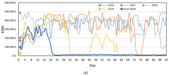
Figure 3. The daily electricity demand (KWh) in Jordan during the movement restriction orders during the ongoing pandemic period over five years: (a) city center; (b) Ashrafiah; (c) Rashadieh.

The half-hourly electrical demand during the ongoing pandemic period (March, April, and May) over five years is shown in Figure 4. Each box plot in Figure 4 shows the distribution of half-hourly electrical demand. In 2020, the median half-hourly electrical demand for the city center was around 180 MWh, and it was the lowest compared to previous years. This is mainly related to the fact that the current COVID-19 pandemic has changed the patterns of our demand behavior. In addition, the movement restrictions which were issued in Jordan during the period between March and May 2020 to contain the spread of COVID-19 [22,23,24] lea to reducing the demand consumption. However, the box plot of 2020 overlaps with other years when the government in Jordan began to ease lockdown measures during May 2020 [22,23,24], as seen in Figure 4. Furthermore, the maximum half-hourly electrical demand in 2020 was around 320 MWh, and it was the lost maximum compared to previous years. The reduction in the maximum half-hourly demand in 2020 was 39%, 37%, 34%, and 33% compared to 2016 to 2019, respectively. The half-hourly electrical demand values, as shown in Figure 4, are distributed between 5 and 55 MWh, which gives a wide range of possible electrical demand scenarios and illustrates the uncertainty in the demand. In Figure 4, the outlier points are increased during 2020, which presents a larger uncertainty level associated with the changing demand consumption behavior due to the current COVID-19 pandemic.

Figure 4. An example, box plot of the half-hourly electricity demand (KWh) in Jordan (city center) during the movement restriction orders during the ongoing pandemic period over five years.

2.2. Autocorrelation Analysis

The previous analysis shows a sign of daily, weekly, monthly, and yearly seasonality over the electrical demand time series. Therefore, this section aims to find the time correlation in the electrical demand time series and then remove it, to show only the demand reduction related to the pandemic. In order to select any correlation between the electrical demand points in the time series, the partial autocorrelation function (PACF) was calculated, as shown in Figure 5. The PACF shows the correlation, corr, between the electrical demand time series at $L_t$ for up to a specific number of lags. The PACF can be mathematically described as in Equation (1) [25,26]. The PACF analysis aims to find the relationship between the two time series points without considering the effect of all time points (lags) in between. In contrast, the autocorrelation function (ACF) is used to find the correlation between the demand time series for different lags (seasonal or calendar patterns). However, the previous demand analysis shows a lack of seasonality in 2020 during the COVID-19 pandemic compared to previous years. Therefore, PACF is used in this section to find any special demand trends, which are not seasonal. To find any correlation or patterns between the time-series points, the partial autocorrelation function (PACF) was calculated over 500 time lags, this is shown in Figures 3–10. The PACF can help to find intra-day and longer correlations that repeatedly occur. The PACF, as shown in Figure 5, presents the correlation between the electrical demand time series and the lagged points, at, say, lag k, after removing all time series points (1, 2, ..., k − 1) between them [27,28].

$${\mathrm{PACF}}_k=\mathrm{corr} \left(L_t, L_{t-k}|L_{t-1},....,L_{t-k-1} \right).$$

(1)

Figure 5. An example partial autocorrelation function (PACF) plot for the electrical demand time series for (a) monthly, (b) weekly, (c) daily, and (d) half-hourly demand in Jordan (city center) during the movement restrictions orders during the ongoing pandemic period over five years.

The significant values of the PACF occurred and repeated at lags 4, 12, and 24 for monthly demand. This shows clear signs of seasonality every 4 months (season) and every year (12 and 24 months). In Figure 5b, the PACF plot for weekly profiles for the March, April and May period over five years shows that significant values occurred and repeated at a number of lags—1, 8, 12, 26, 30 and 40—which showed a clear sign of patterns from week to week, the same week in the previous month and the same week from the previous year. In Figure 5c,d, the PACF plot for daily and half-hourly profiles shows significant values repeated for a number of lags, showing signs of daily pattern and seasonality. Furthermore, the distribution of PACF lags showed a large spike (main lag) that was followed by a damped wave which presented a moving average term. In general, the PACF plot in Figure 5 shows a cut off after lags 5, 1, 40 and 50 for monthly, weekly, daily, and half-hourly demand, respectively. It also shows other significant PACF lags on longer lags, for example between lag 200 and lag 300 for daily demand. However, the distribution of the significant lags does not present a clear seasonality. The significant longer lags between lag 200 and lag 300, as shown in Figure 5c, were randomly distributed with no sign of a large main spike followed by a damped wave, which can present a moving average trend. These randomly distributed lags are likely random salience due to the new events and the impact of the COVID-19 pandemic on the demand profile. Furthermore, the early correlation lags could be due to the demand behavior with tasks that take more than a single time step to complete. Hence, the collected dataset during the COVID-19 pandemic period and PACF plot depicts random behavior and indicates a lack of clear seasonality.

The electrical demand time series with trends or seasonality will affect the analysis of the time series at different time points. In order to eliminate the trends or seasonality impact on the electrical demand time series and to perform accurate analysis of the COVID-19 pandemic’s effects, a stationary electrical demand time-series needs to be generated. The stationary time series will have no trends or seasonality in the demand series. In this section, to generate a stationary electrical demand time series, a seasonal differencing technique will be used. Seasonal difference aims to find the difference between a demand value and the previous demand value from the same season or previous period, as described in Equation (2) [29]. The seasonal differencing process helps to stabilize the mean of the electrical demand time series by eliminating the seasonal and trend effects on the time series.

$${\widehat{L}}_t= L_t-L_{t-s}.$$

(2)

where ${\widehat{L}}_t$ is the differenced series and s is the number of lag seasons or trends. The seasonally differenced profile for the city center electrical demand time series is presented in Figure 6. The differenced series in Figure 6 for monthly, weekly, daily, and half-hourly profiles showed a pattern of demand reduction during 2020 compared to previous years. This is mainly related to that the multiple levels of restrictions, which were issued in Jordan during March and April 2020 [22,23,24]. The initial measures included schools and universities closing, a nationwide curfew, working from home for office employees, and factories working with the limited number of staff or stopping their production, which affected and dramatically changed the patterns of our demand behavior. The economic and social impact of the COVID-19 pandemic on households and businesses in Jordan during this period was significant, which led to reducing the demand consumption. Generally, the impact of the COVID-19 pandemic on electricity demand consumption is presented in this section after removing the seasonality terms, and it showed a strong decline in electricity consumption.

Figure 6. An example for differenced demand series plot for (a) monthly, (b) weekly, (c) daily, and (d) half-hourly demand in Jordan (city center) during the movement restrictions orders period over five years.

2.3. Peak Demand Analysis

Analysis of the daily electrical demand data for the city center, as an example, is presented in Table 1 to present various statistics of the demand data including the maximum, minimum and average values at daily resolutions. A comparison of the daily electrical demand over five years during the movement restrictions orders period (March, April, and May) shows that the maximum, minimum, and average demand in 2020 significantly decreased compared to previous years. For illustration, the peak demand decreased to 1293 MWh in 2020 compared to 2098 MWh in 2016 and 1768 MWh in 2019. The peak demand in 2020 was reduced by 30% and 25% compared to 2017 and 2018, respectively. Furthermore, the minimum and average demand in 2020 was also decreased compared to previous years. For example, the minimum demand in 2020 was 765 MWh compared to 1219 and 1029 MWh for 2018 and 2019, respectively. The average demand in 2020 was reduced by 40% and 37% compared to 2019 and 2017, respectively. In Jordan, the peak demand and demand behavior were directly affected during the initial measures period (March to May 2020), which led to a reduction in the electricity consumption. In addition, as economies tried to recover from the COVID-19 pandemic and the initial measures, many companies and factories in Jordan struggled to pay salaries or retain employees. Furthermore, the unemployment level has increased due to the COVID-19 pandemic, particularly in the informal business sector [22,23,24]. Therefore, the impact of the COVID-19 pandemic continues and will have a long-term effect on the electricity demand pattern for all regions.

Table 1. Summary of the electrical demand between 2016 and 2020 during the movement restrictions orders period (March, April, and May).

	Electrical Demand (MWh)					The Percentage Reduction in Demand in 2020 Compared to Previous Years
	2016	2017	2018	2019	2020	2016	2017	2018	2019
Maximum demand	2098	1839	1735	1768	1293	38%	30%	25%	37%
Minimum demand	1128	1189	1219	1029	765	32%	36%	37%	35%
Average demand	1443	1492	1444	1319	941	35%	37%	35%	40%

3. Load Forecasting Models

In general, the forecasting models are developed to predict the demand profiles and follow the fluctuating in the demand [10,11,12,13,14,15,16]. As illustrated in Section 2, the stochastic and non-smooth behavior of the electrical demand during and after the COVID-19 pandemic increases the challenges of accurately predicting the demand compared to previous years. Normally, point forecasts are used to generate electrical demand with a single estimate value for each time step [11,12]. However, this is mainly limited to the time-series data, the description of the model and the degree of uncertainty in the data. In cases of highly stochastic and unpredicted conditions, a forecast model with the ability to handle new and unpredicted conditions (such as the COVID-19 pandemic) and work under different degrees of uncertainty is required. Therefore, rolling and fixed probabilistic forecast models are developed in this section to predict the electrical demand (half-hourly, daily, weekly, and monthly), $\stackrel{\cdots }{\mathrm{L}}$. The fixed forecast model generates a future demand profile over a specific period, without updating the observation during this period. The rolling forecast model works to generate a future demand profile, and then the model will be updated with new observations after each time step [6,14]. This rolling procedure aims to minimize the forecast error over the prediction horizon period by recalculating and updating the forecast profile using the new real-time measurements and forecast error after each time step.

3.1. Probabilistic Forecast Model

Probabilistic forecasts are estimation models that aim to generate future demand scenarios based on the distribution of the data model [14,16]. In this section, an ensemble forecast model is developed to generate future scenarios of the electricity demand in 2020 as follows:

• The half-hourly demand over the coming day.
• Daily demand over the coming week.
• Monthly demand over the coming year.

The ensemble forecast model aims to handle the inter-dependencies and uncertainty in the data and generate a wider range of forecast model scenarios. To present the volatile and uncertain electrical demand, the hybrid-forecasting model is developed in this section, including Auto Regressive Integrated Moving Average with Exogenous (AIRMX) method and Monte Carlo sampling method (stochastic ARIMAX forecast model). The ARIMAX is described by Equation (3) as a common model for forecasting electrical demand time series [6,15,16,17,18].

$${\stackrel{\cdots }{{\mathrm{L}}_{ }}}_t = {\displaystyle \sum }_{\mathrm{j}=0}^{\mathrm{h}}{\mathrm{A}}_{\mathrm{j}}{\mathrm{X}}_{\mathrm{j}}\left(\mathrm{t}\right)+{\displaystyle \sum }_{\mathrm{i}=1}^{\mathrm{p}}{\mathrm{B}}_{\mathrm{i}}\hat{\mathrm{L}}\left(\mathrm{t}-\mathrm{i}\right)+{\displaystyle \sum }_{\mathrm{i}=1}^{\mathrm{q}}\mathrm{C} \mathrm{Z}\left(\mathrm{t}-\mathrm{i}\right) + \mathrm{E},$$

(3)

where ${\stackrel{\cdots }{{\mathrm{L}}_{ }}}_t$ is the estimation of differenced demand at time t;${\displaystyle \sum }_{\mathrm{i}}^{\mathrm{p}}{\mathrm{B}}_{\mathrm{i}}\hat{\mathrm{L}}\left(\mathrm{t}-\mathrm{i}\right)$ is the autoregressive term with ${\mathrm{p}}^{\mathrm{th}}$ order lag ($\mathrm{AR}\left(\mathrm{p}\right)$ model); ${\displaystyle \sum }_{\mathrm{i}}^{\mathrm{q}}{\mathrm{C}}_{\mathrm{i}}\mathrm{Z} \left(\mathrm{t}-\mathrm{i}\right)$ moving average term with ${\mathrm{q}}^{\mathrm{th}}$ order lag ($\mathrm{MA} \left(\mathrm{q}\right))$; ${\displaystyle \sum }_{\mathrm{j}=0}^{\mathrm{h}}{\mathrm{A}}_{\mathrm{j}}{\mathrm{X}}_{\mathrm{j}}\left(\mathrm{t}\right)$ is the ${\mathrm{A}}^{\mathrm{th}}$ exogenous variables term, and E is a constant value. The p, d, and q order for the ARIMAX model is selected by using the Bayesian information criterion (BIC) matrix computation. The BIC matrix has been computed for the following values—p between 1 and 48, q between 0 and 48, and d between 0 and 5—which can assist in parameter selection in the ARIMAX model for all cases. The BIC matrix results show that the most preferable parameters through lowest BIC are (p, d, q) = (1,1,2), (1,1,2) and (2,1,2). The following exogenous variables, in Table 2, were chosen and used for the suggested ARIMAX model after testing a wide range of possible variables.

Table 2. The exogenous variables for Auto Regressive Integrated Moving Average with Exogenous (ARIMAX) model for half-hourly, daily, and monthly periods.

Testing Period	${\mathbf{X}}_1$	${\mathbf{X}}_2$	${\mathbf{X}}_3$	${\mathbf{X}}_4$	${\mathbf{X}}_5$
Months	The monthly average temperature.	Average of the previous two months demand	Former month demand.	Former year demand in same month.	Stochastic samples of from the monthly demand dataset.
Daily	The daily average temperature.	Average of the previous two days demand	Former day demand.	Former week demand in same day.	Stochastic samples of from the daily demand dataset
Half-hourly	The half-hourly average temperature.	Average of the previous two half hours demand	Former half hour demand.	Former day demand in same half hour.	Stochastic samples of from the half-hourly demand dataset

The stochastic samples of demand data for half-hourly/daily/monthly demand using the Monte Carlo sampling method aim to present the uncertainty in the demand profile and create a number of possible scenarios. Monte Carlo simulation uses a random sampling process to cover the uncertainty of data by providing a range of possible demand scenarios that may capture a range of possible events through the simulation iterations. As previously discussed, the electrical demand analysis shows a weak relation to the historical demand during the pandemic period due to the movement restriction. However, to evaluate the effect of the calendar variables as input variables on the proposed forecast model, the holiday and weekend indicators are tested in addition to other variables (${\mathrm{X}}_1$ to ${\mathrm{X}}_5$), and then the most effective input variables that improve the forecast model performance are chosen. The exogenous variables ${\mathrm{X}}_1$ to ${\mathrm{X}}_5$ are selected based on the trial-and-error tests as input variables for the proposed forecast model, due to the strong relationship between them and current time demand. However, the exogenous variables ${\mathrm{X}}_3$ and ${\mathrm{X}}_4$ can be linked to other time series forecast models such as ARIMA, AR, and seasonal AR, but this will not be the case for ANN. In this paper, different exogenous variables are tested with ANN and ARIMAX and then the most effective input variables that improve the forecast models performance are chosen. Furthermore, adding other exogenous variables such as the size of traffic and factories production (monthly, daily, and half-hourly) can help to improve the forecast error. However, this level of data was not available for the current and previous years, so the stochastic sampling using Monte Carlo sampling aims to cover the uncertainty of data by providing a range of possible demand scenarios. The ARIMA forecast model has been modified to create a number of potential future scenarios using the Monte Carlo sampling method. Firstly, we generate stochastic samples of the electrical demand from a joint probability distribution for the electrical demand with average temperature and time of the half-hour, day and month. Then, the ARIMAX model is used to obtain the forecast scenarios based on the number of demand samples. For sampling the stochastic electrical demand from the probability empirical distribution, a 2D histogram of the demand and the external variables with 48 bins is used.

The stochastic ARIMAX forecast model in this paper uses the real time measurements (actual demand) and the forecast error for each time step to regenerate the future demand profile by recalculating and updating the forecast demand based on these values for the prediction horizon period, the rolling stochastic ARIMAX forecast model is designed to:

• Firstly, predict the electrical demand over the proposed prediction horizon period and generate a future electrical demand profile (let say from t to t + 12).
• Secondly, collect the real-time measurements (actual demand) and calculate the forecast error at time t.
• Thirdly, update the stochastic ARIMAX forecast model using the new observations and real measurements at time t, and then regenerate the future electrical demand profile at each time step t + 1 to t + 12 + 1. Here, the stochastic ARIMAX forecast model is rerun to generate the future demand profile with the new observation.

3.2. ANN Forecast Model

The ANN feedforward model, with two hidden layers and ten neurons in each hidden layer, is developed in this paper to forecast the electrical demand. The main parameters of the ANN model such as the number of layers and input variables are chosen after testing a wide range of possible variables using the trial-and-error approach and then the most effective input variables or parameters that improve the forecast model performance are chosen. In the proposed ANN model, the input variables were similar to ARIMAX and the remaining model parameters can be summarized as follows:

• Training function: Levenberg–Marquardt backpropagation.
• Transfer function: sigmoid function.
• Evaluation criteria: the full squared errors.
• The stopping criteria: once there is no additional development in the error function.

4. Forecast Results

The stochastic ARIMAX forecast model, as described in the previous section, aims to minimize the impact of the stochastic nature of the electrical demand on the forecast performance. The stochastic ARIMAX forecast model was developed as fixed and rolling forecast models to investigate the impact of updating the observation in the forecast model on the forecast performance for electrical demand.

In this section, the stochastic ARIMAX forecast model (fixed and rolling) will be presented and compared to common forecast models ANN [8,13] and ARIMAX [6,27] for electrical demand. However, to evaluate the selected benchmark forecast models, the ARIMAX and ANN are tested and compared to a simple naïve model. The proposed naïve model developed to create the future demand based on the previous year’s demand in the same month, the previous week demand in the same month, and the previous day demand in the same half-hour for monthly, daily, and half-hourly profiles, respectively. The simple naïve model showed a higher forecast error compared to ANN and ARIMAX during the pandemic period with 14%, 11%, and 10% mean absolute percentage error (MAPE) for monthly, daily, and half-hourly profiles, respectively. Therefore, the most effective forecast models (ANN and ARIMAX) were chosen to be the benchmark models. In general, the common forecast models ANN and ARIMAX for electrical demand achieved the best results compared to other benchmark models such as naïve forecast models, especially with the stochastic demand behavior during the pandemic. The stochastic ARIMAX forecast model results in this section are for the average demand scenario. Firstly, the collected data and forecasting model evaluation are presented, then the proposed forecast models are compared. In Section 4.3, the performance of the stochastic ARIMAX forecast model during the COVID-19 pandemic is presented and discussed.

4.1. Data Collection and Forecasting Model Evaluation

As discussed previously, we collected data from the National Electric Power Grid Co (NEPCO) over a five-year period from January 2016 until the end of November 2020. The half-hourly electrical demand data werecollected from three main areas in Jordan: city center, Ashrafiah, and Rashadieh. The collected data were divided into a training dataset (2016 and 2017) and a testing dataset (2018 to 2020). In order to assess and evaluate the performance of the proposed forecast models, it is significant to define and determine the evaluation techniques. In this section, the mean absolute percentage error (MAPE) measures were used, as the most common forecasting evaluation methods. The MAPE is a scale-independency elevation model, which make its ease of interpretation [9,10,11,30]. However, the MAPE is calculated only for the cases when the actual demand is greater than zero, otherwise it will produce undefined values. Therefore, the forecast error is used to avoid this problem and help evaluate the stochastic ARIMAX forecast model performance. The forecast error and MAPE techniques are described in Equations (4) and (5), respectively [31,32].

$$\mathrm{Err} ={\mathrm{L}}_t-{\stackrel{\cdots }{{\mathrm{L}}_{ }}}_t,$$

(4)

$$\mathrm{MAPE} =\frac{100}{\mathrm{T}}{\displaystyle \sum }_{\mathrm{t}=1}^{\mathrm{T}}\left|\frac{{\mathrm{L}}_t-{\stackrel{\cdots }{{\mathrm{L}}_{ }}}_t}{{\mathrm{L}}_t}\right|,$$

(5)

where ${\mathrm{L}}_t$ is the actual electrical demand at time step t; ${\stackrel{\cdots }{{\mathrm{L}}_{ }}}_t$ is the forecasted demand at time step t; t is the current time step, and T is the total steps of the prediction horizon period (total number of observations).

4.2. Overall Comparisons

In this section, the overall MAPE was calculated for each proposed period and presented in Table 3. In general, the stochastic ARIMAX (rolling) outperformed other proposed models and achieved the best forecast model accuracy (MAPE%) overall testing periods. The stochastic ARIMAX (rolling and fixed) outperformed the other two benchmarks, ARIMAX and ANN. From Table 3, it is seen that by involving a stochastic term in the forecast model, the performance is improved compared to the ANN and ARIMAX models, which only use the historical demand data. For example, the overall monthly MAPE during 2019 for the fixed stochastic ARIMAX was 4.6%, compared to 4.9% and 5.9% for ARIMAX and ANN models, respectively. The rolling stochastic ARIMAX helped to decrease the daily MAPE in 2018 by 22.4% and 23.7% for ARIMAX and ANN models, respectively. Furthermore, the high MAPE% occurred during 2020, and this corresponds to the stochastic and non-smooth demand nature due to the COVID-19 pandemic. This is can be explained by the demand analysis introduced in Section 2. However, the stochastic ARIMAX (rolling and fixed) provided the most accurate forecast models compared to ANN and ARIMAX during 2020 and the stochastic term in the proposed forecast model minimizes the impact of the COVID-19 pandemic on forecasts performance. In addition, by updating the forecast model every in rolling stochastic ARIMAX, the forecast performance improved the overall half-hourly, daily, and monthly MAPE during 2020 by 23.3%, 22.5%, and 18.4% compared to the fixed stochastic ARIMAX model, respectively. In general, the forecast error (MAPE) for aggregate demand is normally around 3–4% [10,11,12,33]; however, recently, with the increasing number of renewable energy resources for small and large scales and to use of more electrical vehicles, the forecast error increased up to 6% during normal conditions based on the nature of the power networks [16,31]. In addition, the MAPE for demand with stochastic behavior similar to our case in this paper is achieved at around 10% [9,16].

Table 3. The overall mean absolute percentage error (MAPE) over each of the testing periods.

Testing Period		Stochastic ARIMAX (Fixed)	Stochastic ARIMAX (Rolling)	ARIMAX	ANN
Months	2018	5.1%	4.3%	5.2%	5.7%
	2019	4.6%	4.1%	4.9%	5.9%
	2020	6.5%	5.3%	8.9%	8.1%
Daily (March–May)	2018	5.9%	4.5%	5.8%	5.9%
	2019	5.2%	4.1%	5.5%	5.8%
	2020	7.1%	5.5%	8.2%	9.0%
Half-hourly (March–May)	2018	5.8%	4.6%	6.0%	5.9%
	2019	5.1%	4.3%	5.7%	5.6%
	2020	7.3%	5.6%	9.3%	9.8%

4.3. Stochastic ARIMAX (Rolling Model): Forecast Error Analysis

The main aim of developing a rolling stochastic ARIMAX forecast model is to improve the forecast performance by capturing the non-smooth electrical demand nature and creating a number of future electrical demand scenarios to feed the forecast model. Table 2 shows that the proposed rolling stochastic ARIMAX forecast model presented a significant improvement compared to all other forecast models. Therefore, this section presents the rolling stochastic ARIMAX forecast model results. Firstly, the rolling stochastic ARIMAX forecast model profiles are generated for each testing period and then the average demand scenario is plotted, as illustrated in Figure 7. From Figure 7, the rolling stochastic ARIMAX forecast model captures all main peaks and the prediction demands were around the actual demand value. The averaged demand scenarios from the rolling stochastic ARIMAX forecast showed small deviations around the actual demand at each time step. During the COVID-19 pandemic period (March to May 2020), the stochastic and rolling process helped to minimize the forecast error and capture the actual demand, as shown in Figure 8. The results in Figure 8 presents the calculated forecast error at each time step. The variation in the forecast error results in Figure 8 is mainly related to the high non-smooth nature of the demand. Furthermore, Figure 9 presents the histogram of the forecast error for the rolling stochastic ARIMAX forecast model for all testing periods. The rolling stochastic ARIMAX forecast model takes into account the uncertainty in demand data by updating the model variables after every time step to improve the forecast performance. The result shows the forecast error values for all testing periods were normally distributed around the zero value, as presented in Figure 9. The histogram plots for the forecast errors showed that the high number of instances are clustered around zero error, which means that the forecast model achieved the highest performance and no bias in the forecast error results, which also means the minimum uncertainty (error) in the forecast profile. In order to evaluate the forecast error and investigate the availability of any seasonality and trend in the forecast error, the ACF of the forecast error series is plotted in Figure 10. The ACF aims to measure the relationship between the historical errors and how the errors in the time series are correlated. The ACF aims here to check if there are any seasonal patterns in the error profiles. The forecast error series shows highly volatile behavior without any repetition in the significant lags of ACF. This shows that there are no signs of trend or seasonality, which makes it difficult to improve the forecast accuracy further.

Figure 7. Results of rolling stochastic ARIMAX forecast model with the average demand scenario for a (a) monthly, (b) daily, and (c) half-hourly testing period in Jordan (city center).

Figure 8. Forecast error results of rolling stochastic ARIMAX forecast model with the average demand scenario for a (a) monthly, (b) daily, and (c) half-hourly testing period in Jordan (city center).

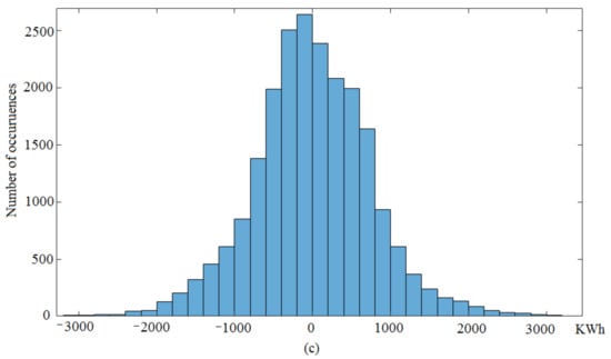
Figure 9. Histogram for the forecast error results of rolling stochastic ARIMAX forecast model with the average demand scenario for (a) monthly, (b) daily, and (c) half-hourly testing period in Jordan (city center).

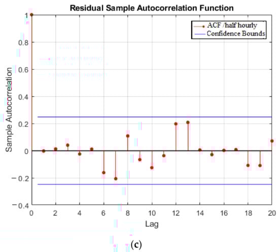
Figure 10. Autocorrelation function (ACF) plots for the forecast error results of rolling stochastic ARIMAX forecast model with the average demand scenario for a (a) monthly, (b) daily, and (c) half-hourly testing period in Jordan (city center).

5. Conclusions

The multiple levels of movement restrictions to contain the spread of COVID-19 have significantly affected the electricity demand consumption’s and the demand profile’s nature and pattern. As economies try to recover from the COVID-19 pandemic, the electricity demand starts to slowly return to the pre-pandemic values. However, the impact of the COVID-19 pandemic continues, and will have a long-term effect on our lives. Thus, understanding electricity demand changes and their impacts on load forecasting is important to maintain a reliable operation of the electrical grid. Unlike previous studies that covered only the start of the pandemic period, this paper aimed to examine and analyze electrical demand data over a longer period of time. The electrical demand analysis for three regions showed a clear sign of peak and demand reduction due to the pandemic. Unlike previous studies, the demand analysis process in this paper is developed based on eliminating the times series correlation, trends, and seasonality impact on the demand analysis to cover only the pandemic’s impacts. Finally, a rolling stochastic ARIMAX forecast model has been developed to improve the forecast performance by capturing the non-smooth electrical demand nature and creating a number of future electrical demand scenarios to feed the forecast model. The proposed forecast model outperformed the benchmark forecast model ARIMAX and ANN.

References

- Agdas, D.; Barooah, P. Impact of the COVID-19 pandemic on the U.S. electricity demand and supply: An early view from data. IEEE Access 2020, 8, 151523–151534. [Google Scholar] [CrossRef]
- Baker, S.; Bloom, N.; Davis, S.; Terry, S. COVID-induced economic uncertainty. Natl. Bur. Econ. Res. Pap. 2020. [Google Scholar] [CrossRef]
- Bui, Q.; Wolfers, J. Another way to see the recession: Power usage is way Down. New York Times. 8 April 2020. Available online: https://www.nytimes.com/interactive/2020/04/08/upshot/electricity-usage-predictcoronavirusrecession.html (accessed on 28 January 2021).
- Abu-Rayash, A.; Dincer, I. Analysis of the electricity demand trends amidst the COVID-19 coronavirus pandemic. Energy Res. Soc. Sci. 2020, 68, 101682. [Google Scholar] [CrossRef] [PubMed]
- Narajewski, M.; Ziel, F. Changes in Electricity Demand Pattern in Europe Due to COVID-19 Shutdowns. IAEE Energy Forum/Covid-19 Issue. arXiv 2020, arXiv:200414864N. [Google Scholar]
- Alasali, F.; Haben, S.; Becerra, V.; Holderbaum, W. Day-ahead industrial load forecasting for electric RTG cranes. J. Mod. Power Syst. Clean Energy 2018, 6, 223–234. [Google Scholar]
- Aneiros, G.; Vilar, J.; Raña, P. Short-term forecast of daily curves of electricity demand and price. Int. J. Electr. Power Energy Syst. 2016, 80, 96–108. [Google Scholar] [CrossRef]
- Alasali, F.; Haben, S.; Becerra, V.; Holderbaum, W. Optimal Energy Management and MPC Strategies for Electrified RTG Cranes with Energy Storage System. Energies 2017, 10, 1598. [Google Scholar] [CrossRef]
- Alasali, F.; Haben, S.; Holderbaum, W. Energy management systems for a network of electrified cranes with energy storage. Int. J. Electr. Power Energy Syst. 2019, 106, 210–222. [Google Scholar] [CrossRef]
- Santra, A.S.; Lin, J.-L. Integrating Long Short-Term Memory and Genetic Algorithm for Short-Term Load Forecasting. Energies 2019, 12, 2040. [Google Scholar] [CrossRef]
- Park, R.-J.; Song, K.-B.; Kwon, B.-S. Short-Term Load Forecasting Algorithm Using a Similar Day Selection Method Based on Reinforcement Learning. Energies 2020, 13, 2640. [Google Scholar] [CrossRef]
- Acakpovi, A.; Ternor, A.T.; Asabere, N.Y.; Adjei, P.; Iddrisu, A.-S. Time series prediction of electricity demand using Adaptive Neuro-Fuzzy Inference Systems. Math. Probl. Eng. 2020, 2020, 4181045. [Google Scholar] [CrossRef]
- Wei, D.; Wang, J.; Ni, K.; Tang, G. Research and Application of a Novel Hybrid Model Based on a Deep Neural Network Combined with Fuzzy Time Series for Energy Forecasting. Energies 2019, 12, 3588. [Google Scholar] [CrossRef]
- Prado, F.; Minutolo, M.C.; Kristjanpoller, W. Forecasting based on an ensemble Autoregressive Moving Average—Adaptive neuro—Fuzzy inference system—Neural network—Genetic Algorithm Framework. Energy 2020, 197. [Google Scholar] [CrossRef]
- Sowinski, J. The Impact of the Selection of Exogenous Variables in the ANFIS Model on the Results of the Daily Load Forecast in the Power Company. Energies 2021, 14, 345. [Google Scholar] [CrossRef]
- Selim, M.; Zhou, R.; Feng, W.; Quinsey, P. Estimating Energy Forecasting Uncertainty for Reliable AI Autonomous Smart Grid Design. Energies 2021, 14, 247. [Google Scholar] [CrossRef]
- Abu Dyak, A.; Abu-Lehyeh, E.; Kiwan, S. Assessment of Implementing Jordan’s Renewable Energy Plan on the Electricity Grid. Jordan J. Mech. Ind. Eng. 2017, 11, 113–119. [Google Scholar]
- Arfoa, A. Long-Term Load Forecasting of Southern Governorates of Jordan Distribution Electric System. Energy Power Eng. 2015, 7, 242–253. [Google Scholar] [CrossRef]
- AbuAl-Foul, B. Forecasting Energy Demand in Jordan Using Artificial Neural Networks. Top. Middle East. Afr. Econ. 2012, 14, 473–478. [Google Scholar]
- Badran, I.; El-Zayyat, H.; Halasa, G. Short-Term and Medium-Term Load Forecasting for Jordan’s Power System. Am. J. Appl. Sci. 2008, 5, 763–768. [Google Scholar] [CrossRef]
- Momani, M.; Alrousan, W.; Alqudah, A. Short-term load forecasting based on NARX and radial basis neural networks approaches for the Jordanian power grid. Jordan J. Electr. Eng. 2016, 2, 81–93. [Google Scholar]
- Pedersen, A. Socio-Economic Framework for COVID-19 Response in Jordan; United Nations in Jordan: Amman, Jordan, 2020. [Google Scholar]
- UNDP. COVID-19 Impact on Households in Jordan; UNDP: Amman, Jordan, 2020. [Google Scholar]
- Kebede, T.; Stave, S.; Kattaa, M.; Prokop, M. Impact of the COVID-19 pandemic on enterprises in Jordan. Int. Labour Organ. 2020, in press. [Google Scholar]
- Deb, C.; Zhang, F.; Yang, J.; Lee, S.; Shah, K. A review on time series forecasting techniques for building energy consumption. Renew. Sustain. Energy Rev. 2017, 74, 902–924. [Google Scholar] [CrossRef]
- Chadsuthi, S.; Modchang, M.; Lenbury, Y.; Iamsirithaworn, S.; Triampo, W. Modeli-ng seasonal leptospirosis transmission and its association with rainfall and temperature in Thailand using time-series and ARIMAX analyses. Asian Pac. J. Trop. Med. 2012, 5, 539–546. [Google Scholar] [CrossRef]
- Amini, M.; Kargarian, A.; Karabasoglu, O. ARIMA-based decoupled time series forecasting of electric vehicle charging demand for stochastic power system operation. Electr. Power Syst. Res. 2016, 140, 378–390. [Google Scholar] [CrossRef]
- Cui, H.; Peng, X. Short-term city electrical load forecasting with considering tempe-rature effects: An improved ARIMAX model. Math. Probl. Eng. 2015. [Google Scholar] [CrossRef]
- Munkhammara, J.; Widna, J.; Rydnb, J. On a probability distribution model comb-ining household power consumption, electric vehicle home-charging and photovoltaic power production. Appl. Energy 2015, 142, 135–143. [Google Scholar]
- Nusair, K.; Alasali, F. Optimal Power Flow Management System for a Power Network with Stochastic Renewable Energy Resources Using Golden Ratio Optimization Method. Energies 2020, 13, 3671. [Google Scholar] [CrossRef]
- Klingler, A.; Teichtmann, L. Impacts of a forecast-based operation strategy for grid-connected PV storage systems on profitability and the energy system. Solar Energy 2017, 158, 861–868. [Google Scholar]
- Hernandez, L.; Baladrón, C.; Aguiar, J.; Carro, B.; Sanchez-Esguevillas, A.; Lloret, J. Short-Term Load Forecasting for Microgrids Based on Artificial Neural Networks. Energies 2013, 1385–1408. [Google Scholar] [CrossRef]
- Jalalkamali, A.; Moradi, M.; Moradi, N. Application of several artificial intelligence models and ARIMAX model for forecasting drought using the Standardized Precipitation Index. Int. J. Environ. Sci. Technol. 2015, 12, 1201–1210. [Google Scholar] [CrossRef]
Publisher’s Note: MDPI stays neutral with regard to jurisdictional claims in published maps and institutional affiliations. |
© 2021 by the authors. Licensee MDPI, Basel, Switzerland. This article is an open access article distributed under the terms and conditions of the Creative Commons Attribution (CC BY) license (http://creativecommons.org/licenses/by/4.0/).