Cooling Effect of Different Land Cover Types: A Case Study in Xi’an and Xianyang, China

Abstract

One of the climate problems caused by rapid urbanization is the urban heat island effect, which directly threatens the human survival environment. In general, some land cover types, such as vegetation and water, are generally considered to alleviate the urban heat island effect, because these landscapes can significantly reduce the temperature of the surrounding environment, known as the cold island effect. However, this phenomenon varies over different geographical locations, climates, and other environmental factors. Therefore, how to reasonably configure these land cover types with the cooling effect from the perspective of urban planning is a great challenge, and it is necessary to find the regularity of this effect by designing experiments in more cities. In this study, land cover (LC) classification and land surface temperature (LST) of Xi’an, Xianyang and its surrounding areas were obtained by Landsat-8 images. The land types with cooling effect were identified and their ideal configuration was discussed through grid analysis, distance analysis, landscape index analysis and correlation analysis. The results showed that an obvious cooling effect occurred in both woodland and water at different spatial scales. The cooling distance of woodland is 330 m, much more than that of water (180 m), but the land surface temperature around water decreased more than that around the woodland within the cooling distance. In the specific urban planning cases, woodland can be designed with a complex shape, high tree planting density and large planting areas while water bodies with large patch areas to cool the densely built-up areas. The results of this study have utility for researchers, urban planners and urban designers seeking how to efficiently and reasonably rearrange landscapes with cooling effect and in urban land design, which is of great significance to improve urban heat island problem.

1. Introduction

The urban heat island effect refers to a phenomenon where urban temperature is higher than in the surrounding suburbs and villages [1], which has a strong negative impact on the climate and environment [2,3,4,5]. Natural surfaces are being replaced by cement, asphalt and other artificial impervious surfaces as a result of the rapid expansion of urban space with the urbanization of the world in the 21st century. Thus, the thermal environment of urban space is changed due to the different underlying surface properties. Meanwhile, the more rural population usually migrates to the city, which further causes an increase in heat emissions, indirectly promotes the process of infrastructure construction and industrialization, and aggravates the urban heat island effect [6]. Facing the threat of the heat island effect, researchers have been looking for solutions for many years. Some urban buildings used reflective materials to alleviate the high temperature [7,8], while some used the covering green plants on the roof (also called “green roof”) [9,10,11]. Some studies combined with natural conditions to identify ventilation corridors within the city to alleviate the heat island effect [12,13,14,15], or use seawater [16]. However, these methods have certain limitations. For example, the cooling effect of reflective materials is susceptible to climate, location and other conditions, and may even lead to the reduction in rainfall, surface runoff and soil moisture in arid areas [17,18], while urban ventilation corridors may require an appropriate wind environment.

Existing studies have shown that some land cover types, such as vegetation and water are cold sources in sunny summer compared with other urban construction land cover, which can significantly regulate the urban microclimate to achieve a cooling effect. This phenomenon is called the cold island effect [19,20,21]. Thus, using vegetation and water to alleviate the heat island effect is thought to be simpler and more efficient compared with other cooling methods. At present, related research mainly includes the field measurement method [22,23,24], numerical simulation method [25,26] and remote sensing monitoring method [27,28]. The field measurement method collects meteorological data through weather stations or observation points, and analyzes the cooling effect of vegetation and water with measured data such as temperature, humidity and wind speed. This method has a good time continuity, but the number of samples is limited, and the results are relatively rough [29]. The numerical simulation method simulates the thermal environment by establishing a mathematical model. Though this method can be more accurate for quantitative analysis, it has uncertainty in parameter settings and is easily affected by subjective factors of researchers. Remote sensing data have the characteristics of large coverage, strong continuity, short update cycle and abundant information. Land surface temperature (LST) and land cover (LC) information can easily be obtained from this data [30,31,32,33], which have been widely used in thermal environment research [34,35,36,37,38]. The research on cooling effect based on remote sensing data mostly focuses on the spatial structure or surrounding environment of land cover types with cooling effect, and discusses their influence on cooling effect, which provides a theoretical basis for the research on cooling effect [27,39,40,41,42,43]. However, with the change in spatial structure and distribution, these land cover types would have different effects on LST change. In addition, the cooling effect varies with the change in geographical location and climatic conditions, and the research results may not be suitable for application in other regions [44,45,46]. Therefore, it is still hard to determine the ideal configuration to achieve the cooling effect, and it is still of great importance to conduct relevant researches in more typical areas.

In fact, most of the existing research focused on large cities in developed regions, while other developing cities with similar problems have received little attention, especially the relatively backward western China. In this study, Xi’an, Xianyang and Xi Xian New Area were selected as typical study areas, and the following issues were studied: (1) influence of different land cover types on land surface temperature change; (2) analysis of the cooling effect of land cover; (3) the influence of spatial structure and distribution of land cover on land surface temperature. To identify the LC types that affect the change in LST, we used the grid-based method to test the correlation between the proportion of different LC types and the LST. The cooling effect of LC was discussed by calculating the cooling distance and intensity, and the influence of landscape configuration on LST was analyzed from the perspective of area, shape and spatial distribution by using a landscape index. Based on these discussions, the optimal landscape configuration needed to achieve the ideal cooling effect in the region was explored, which is helpful for future regional planning.

2. Materials and Methods

2.1. Study Area

Xi’an (107.40°–109.49° E, 33.42°–34.45° N) is the capital city of Shaanxi Province. Its urban areas include Beilin, Lianhu, Xincheng, Yanta, Weiyang, Baqiao districts, and some towns in Chang’an district. Xianyang (107.63°–109.17° E, 34.15°–35.57° N) is close to the northwest of Xi’an, and the main urban areas are Qindu and Weicheng districts. The Xi Xian New Area is located between the main urban areas of Xi’an and Xianyang, with a north–south distribution. Apart from the overlapping parts with Xi’an and Xianyang, Xi Xian New Area also involves some towns of Huyi district, Jingyang district and Xingping City. Xi’an is the economic center of western China. In 2018, the National Development and Reform Commission of China and the Ministry of Housing and Urban-Rural Development issued Guanzhong Plain Urban Agglomeration Development Planning to promote the construction of Xi’an as a national central city. Xianyang is the birthplace of Chinese culture adjacent to Xi’an. In 2014, the State Council approved the establishment of the Xi Xian New Area, which promoted the deep integration of Xi’an and Xianyang, accelerating the process of urbanization in the region. By the end of 2018, the total number of permanent residents in Xi’an and Xianyang reached 14,369,800. Rapid urbanization has led to climate change. In July 2017, Xi’an was ranked the seventh hottest city in China during summer in the official list released by the China Meteorological Administration for the first time. Therefore, it is necessary to find a reasonable urban planning scheme to alleviate the urban heat island effect in the region. The study area covers 1980.08 km², belonging to a warm temperate semi-humid monsoon climate, with hot summers (Figure 1). The study area is the economic center of Shaanxi Province and Guanzhong urban agglomeration, which has important strategic significance for the future development of northwest China.

2.2. Data Source

The remote sensing images used in this study were downloaded from USGS. The imaging time is summer, because the urban heat island effect is the most significant in this season. The Landsat-8 (OLI/TIRS) data were acquired on 29 August 2019, and the Landsat-5 TM data were acquired on 4 June 2011. The path/row number of the two images is 127/36. The downloaded images were Landsat Collection 1 Level-1 data, and radiometric calibration and atmospheric correction were performed in ENVI 5.3. Vector map data used in the study came from China National Geographic Information Public Service Platform.

2.3. LST Retrieval

Using remote sensing data to obtain land surface temperature is a very mature technology, especially for Landsat images. Deriving from the heat radiation transfer equation, the single-window algorithm was used to retrieve the LST in the study area [47]. The thermal infrared band of images (band 10 in Landsat-8 OLI/TIRS, and band 6 in Landsat-5 TM) was used for calculation, and the main methods are as follows

$$T_S=\frac{\left(a\left(1-C-D\right)+\left(b\left(1-C-D\right)+C+D\right)T_a-D{T}_b\right)}{C}$$

$$C=\epsilon \tau$$

$$D=\left(1-\tau \right)\left(1+\left(1-\epsilon \right)\tau \right)$$

where $T_S$ is the real land surface temperature (K), and a and b are constants, which are −67.355351 and 0.458606, respectively. The $\epsilon$ is the surface emissivity, $\tau$ is the atmospheric transmittance of $T_a$, $T_a$ is the pixel brightness temperature detected by the sensor, and $T_b$ is the mean atmosphere applied temperature.

2.4. LC Classification

In this study, the visual interpretation method was used to select classification samples, and the support vector machine supervised classification method was used to classify the LC types through the bands near-infrared, red and green of Landsat-8 data in 2019. In the classification process, Google earth images were compared with the image to improve the accuracy of sample selection, because it has a higher resolution. The study area was divided into five categories, namely construction land, water, green space 1, green space 2 and “other” (

Table 1. Land cover types and detailed description.

Type	Description
Construction land	Artificial impervious surfaces such as buildings, roads, parking lots, squares and so on
Water	All water bodies such as rivers, lakes, ponds, wetlands
Green space 1	Grassland, farmland and other areas covered by vegetation without canopy
Green space 2	Areas covered by canopy vegetation such as forests and shrubs
Other	Bare land and cultivated land with sparse vegetation

), and the LC classification result from the summer of 2019 was obtained. This study evaluates the accuracy of the classification results by comparing the consistency of LC classification and reference data in the same position. In ArcGIS 10.2, 500 random points were created in the study area and converted to kml files that can be opened in Google Earth. By comparing the classification results at sample points with the Google earth image that is closest to the date of remote sensing data acquisition, the overall accuracy of LC classification is 84% (

Table A1. Contingency table.

	Google Earth Image	Construction Land	Water	Green Space 1	Green Space 2	Other
LC Classification Result
Construction land		212	1	15	18	3
Water		1	8
Green space 1		13		78	3	1
Green space 2		14		7	107	1
Other		3				15
OA (%)		84

).

2.5. Spatial Analysis

2.5.1. Spatial Pattern of LST

Based on the image data of 2019, the results of LC classification and LST were obtained. Shaanxi Province officially approved the construction of the Xi Xian New Area in 2011, which promoted the urbanization process. Therefore, the image data of 2011 were used to obtain the results of LST and construction land distribution, then the spatial changes in LST and urban expansion from 2011 to 2019 were discussed. Due to the different acquisition times of the two images, the result of LST cannot be compared immediately. Therefore, it is necessary to standardize this result and classify the standardized result (

Table 2. Classification of land surface temperature (LST).

Level Code	LST Level	Description
1	Extremely low-temperature zone	$T$$<T_{mean}$$-2.5T_{Std}$
2	Low-temperature zone	$T_{mean}$$-2.5T_{Std}$$<T$$<T_{mean}$$-1.5T_{Std}$
3	Sub-middle temperature zone	$T_{mean}$$-1.5T_{Std}$$<T$$<T_{mean}$$-0.5T_{Std}$
4	Middle-temperature zone	$T_{mean}$$-0.5T_{Std}$$<T$$<T_{mean}$$+0.5T_{Std}$
5	Sub-high-temperature Zone	$T_{mean}$$+0.5T_{Std}$$<T$$<T_{mean}$$+1.5T_{Std}$
6	High-temperature zone	$T_{mean}$$+1.5T_{Std}$$<T$$<T_{mean}$$+2.5T_{Std}$
7	Extremely high-temperature zone	$T$$>T_{mean}$$+2.5T_{Std}$

). In the table, $T_{mean}$ is the average value of standardized LST, and $T_{Std}$ is the standard deviation of standardized LST. The change in different LST levels was described by the LST level transfer matrix. The specific method is as follows

$$L_{ij}=\left[\begin{array}{cccc}{L}_{11}& L_{12}& \dots & L_{1n}\\ L_{21}& L_{22}& \cdots & L_{2n}\\ ⋮& ⋮& \ddots & ⋮\\ L_{n1}& L_{n2}& \cdots & L_{nn}\end{array}\right]$$

where L is the area of each LST level, i and j are the LST levels for 2011 and 2019, respectively, and n is the total number of LST levels.

2.5.2. The Relationship between LC and LST

The influence of LC on LST change was explored from different spatial scales by setting grids of different sizes. The specific method is to calculate the proportion of each LC type and mean LST in each grid, and then the correlation between the five kinds of LC density and the average LST is analyzed. At present, there is still controversy regarding the setting of grid size. Song et al. [48] found that 660 × 660 m and 720 × 720 m grids were suitable, Myint et al. [49] suggested 210 × 210 m and 270 × 270 m grids, and Estoque et al. [50] suggested 210 × 210 m and 240 × 240 m grids. Based on these results, Hou et al. [51] chose 210 × 210 m, 450 × 450 m and 690 × 690 m, and achieved ideal results. Combined with previous research experience and the field situation of the study area, the grid sizes of 210 × 210 m, 450 × 450 m and 660 × 660 m were selected, and then the influence of different LC types on LST was identified by using the grids of different sizes as the research units.

2.5.3. Detection of Cooling Distance

After the correlation analysis between LC density and LST, LC types with cooling effect can be identified. Distance analysis was carried out for these LC types, and pixels within a certain range around them were extracted as the results of distance analysis. These pixels stored the information of the distance between themselves and these LC types. The distance results were overlapped with the LST and LC classification results, and each pixel contains three pieces of information: LST, LC types and the distance to each LC type with cooling effect. According to the information of these pixels, the mean LST of each LC type without cooling effect at different distances was counted. It can be determined that the farther away from the LC types with cooling effect within a certain distance, the higher corresponding LST in the surrounding environment. Taking the position of the first inflection point where the rising trend of LST disappears as the cooling distance, and the correlation analysis of LST and distance within the cooling distance was carried out. Based on the above method, the influence range of LC types with cooling effect on LST can be determined. At the same time, the difference between the average LST of the LC with cooling effect and the average LST at the maximum cooling distance was defined as the cooling intensity, and then the influence degree of these LC types on the LST was determined.

2.5.4. Landscape Analysis

Landscape index is a commonly used analysis method in thermal environment research [20,21,27,41], and the influence of area, shape and spatial distribution of LC on LST change has been found. Since the LC types that have a significant impact on LST have been identified, their relationship with LST can be immediately analyzed from the perspective of the landscape index. For the study of landscape-scale, more consideration is given to the combination and configuration of different types of LC. The previous grid-based analysis scale is not applicable because it is too small. At the same time, it should also be considered that the strong heat emission in urban areas with large building density and a dense population may affect the cooling effect [52,53]. Therefore, the study area was divided into 1 × 1 km grids, and the largest patch index (LPI), aggregation index (AI), mean patch shape index (Shape_MN) and mean patch area index (Area_MN) were selected from the perspective of patch types to discuss landscape configuration, because these indices can describe the overall spatial characteristics of each land cover type in a specific area. Area_MN and Shape_MN, respectively, describe the average level of size and shape complexity of the same type of patch. The LPI represents the proportion of the largest patch area in the sum of all patch areas in the same type of patch, while AI represents the aggregation degree. By calculating these indices in each grid, the area, shape and spatial relationship of patches of each LC type can be clearly described. Then, the average LST of each grid was calculated, and the correlation between each landscape index of different LC types and the mean LST was analyzed to explore the influence of landscape configuration on LST.

3. Results

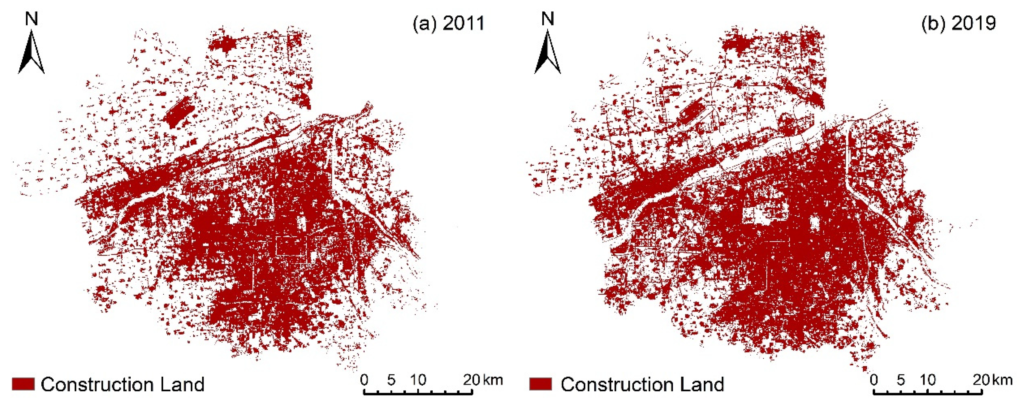
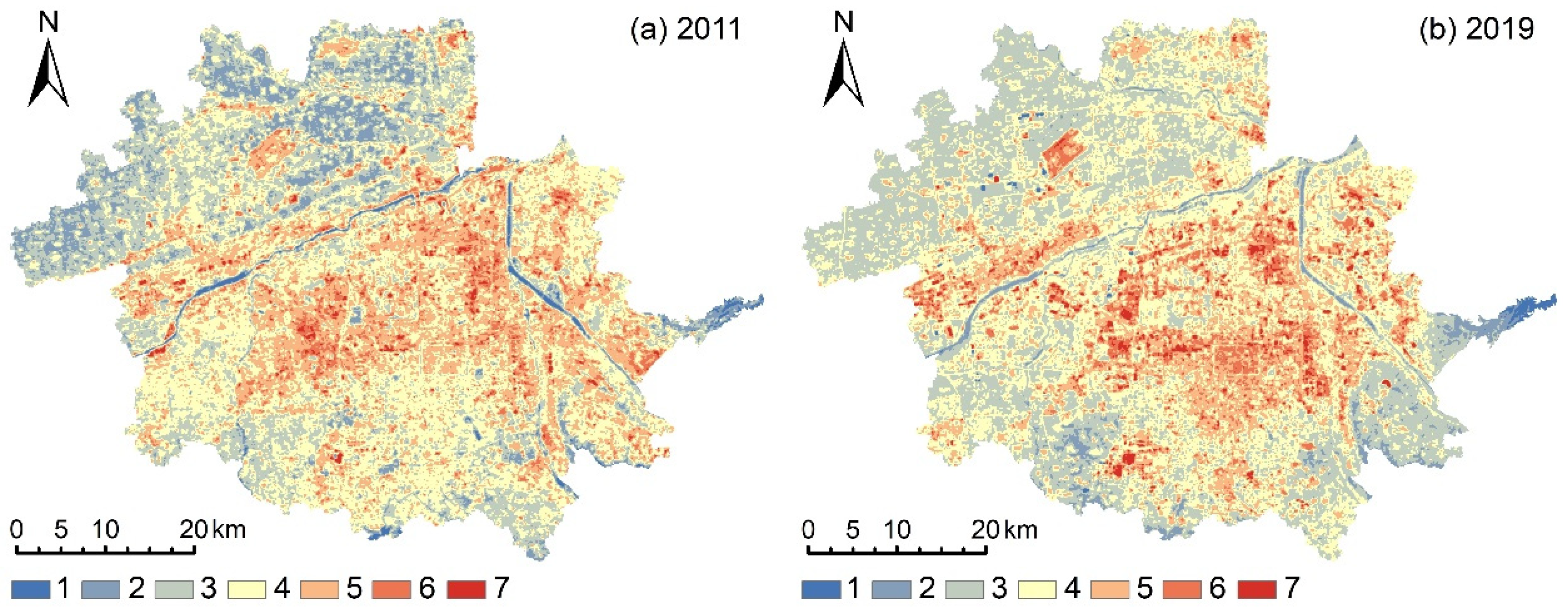
3.1. Land Cover and LST Distribution

The LST and LC types of the study area were obtained from the image of 2019, and the LST and the distribution of construction land were gained through the image data in 2011, so as to analyze the urban expansion and LST rise from 2011 to 2019. The results of LST and LC classification in 2019 were shown in Figure 2. In 2019, the proportion of construction land, “other”, green space 1, green space 2 and water in the total area of the study area was 49.97%, 3.32%, 19.17%, 25.94% and 1.59%, respectively, and the average LST was 33.62, 31.87, 31.20, 30.11 and 28.65 °C, respectively. The area of construction land is the largest, accounting for half of the study area. Green space 2 has the second largest area, mainly including urban greening and fruit trees planted in farmland. Comparisons of construction land distribution and LST between 2011 and 2019 were shown in Figure 3 and Figure 4. The results show that the area of construction land in the study area was 803.32 km² in 2011, and rose to 988.70 km² in 2019, with a growth rate of 23%. The average LST in the study area was 28.35 °C in 2011 and 32.10 °C in 2019. Statistics on changes in LST levels from 2011 to 2019 (

Table 3. LST levels transfer matrix.

	Area in 2019 (km2)	1	2	3	4	5	6	7	Sum
Area in 2011 (km2)
1		2.23	7.63	2.30	0.50	0.13	0.02	0.05	12.86
2		2.71	14.38	88.34	31.70	4.02	0.33	0.42	141.89
3		1.44	17.02	255.95	178.15	22.67	2.41	1.37	479.01
4		0.54	8.73	190.38	359.10	180.82	21.21	2.98	763.76
5		0.12	2.25	67.27	162.35	158.35	73.78	7.28	471.39
6		0.06	0.68	12.96	26.21	21.79	23.47	11.80	96.97
7		0.00	0.09	1.46	2.58	2.27	1.97	5.82	14.20
sum		7.10	50.78	618.65	760.58	390.04	123.20	29.72

), the area below the low-temperature zone decreased from 154.75 to 57.88 km², most of which moved to higher temperature levels. The most significant change was the low-temperature zone, with an area reduction of 64.21% compared with that in 2011. Among the reduced areas, 88.34 and 31.70 km² were transformed into sub-middle and middle-temperature zones, respectively. The area of the extremely low-temperature zone and the extremely high-temperature zone decreased by 44.77% and increased by 109.36%, respectively, compared with 2011, but only formed a small portion of the study area. Overall, the Xi’an, Xianyang urban built-up area significantly expanded, and the LST also significantly increased. Thus, it is urgent to study the cooling effect in this area to improve the thermal environment.

3.2. Relationships between Land Cover Density and LST

Based on the results of LC classification and LST in 2019, LC types that significantly affect LST changes at different scales were identified. In three different sizes of grid, the correlation analysis of the proportion of each LC type and the mean LST was carried out (Figure 5). Since the construction land is mainly artificial impervious surfaces such as buildings and roads, and has strong heat absorption capacity, the proportion of construction land is positively correlated with LST. Additionally, with the increase in grid size, the correlation is gradually enhanced. In contrast, the proportion of green space 2 was negatively correlated with mean LST, and this correlation also increased with the increase in grid size. The area proportion of water is also negatively correlated with LST, especially in the size of 210 × 210 m grid, where the correlation is even higher than in green space 2. However, unlike construction land and green space 2, their correlation gradually decreases with the increase in grid size, and the R² at 660 m grid size dropped to 0.2979. In addition, green space 1 and “other” have no effect on the change in LST.

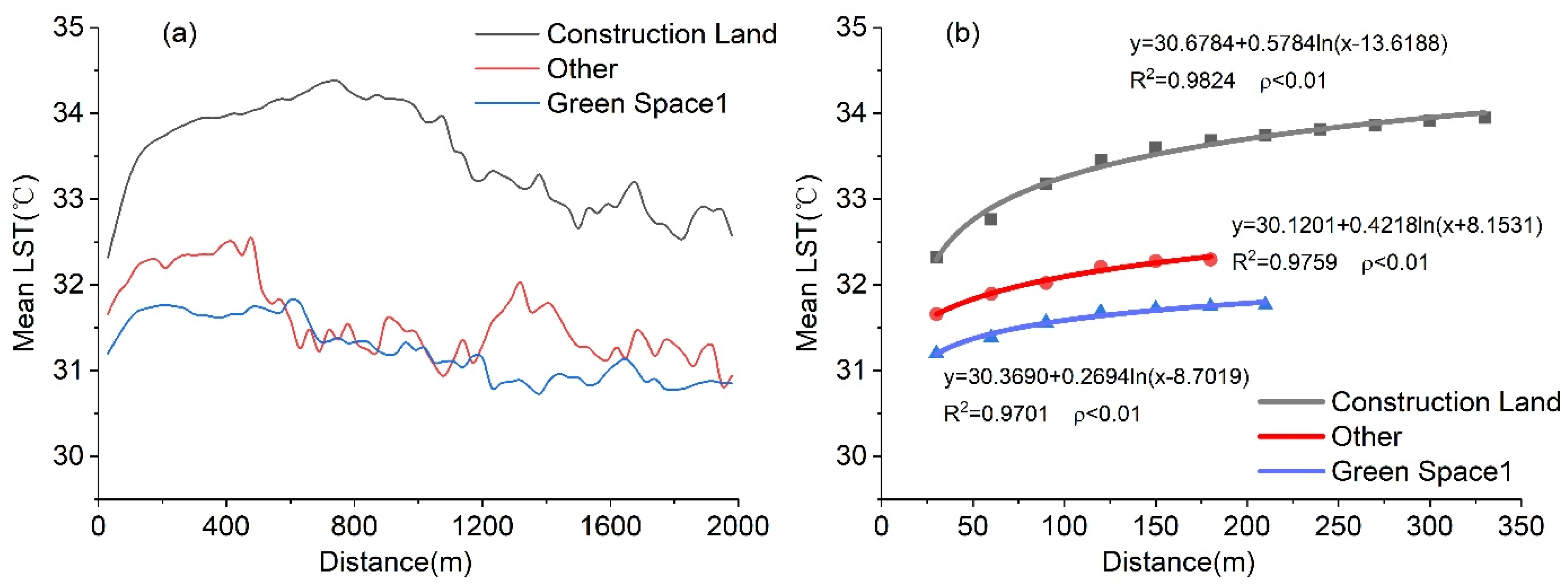
3.3. Cooling Distance Analysis

Previous results showed that green space 2 and water have an obvious cooling effect, but their specific cooling capacity is not clear. Therefore, the results of LC and LST in 2019 were used to explore the cooling distance and intensity of these LC types. The results of the cooling distance analysis showed that, within the cooling distance, with the increasing distance from green space 2 and water, the mean LST of construction land, “other” and green space 1 has a raised trend (Figure 6 and Figure 7). The fitting results of average LST and distance within the cooling range were very ideal (R² > 0.97). The LST of construction land rises to the inflection point when the distance from the green space 2330 m, and the inflection points of “other” and green space 1 appear at 180 and 210 m, respectively. The LST of construction land rises to the inflection point when the distance from the water bodies 180 m, and the inflection points of “other” and green space 1 appear at 150 and 210 m, respectively. Green space 2 has a larger cooling distance than water, especially when the construction land is cooled, which is 150 m longer than that of water. However, the mean LST of construction land, “other” and green space 1 increased by 3.84, 2.19 and 1.66 °C, respectively, in the cooling range of green space 2, and these values were 4.32, 3.94 and 2.93 °C, respectively, in the cooling range of water. Thus, the water has a stronger cooling intensity.

3.4. Relationship between Landscape and LST

From the above results, it can be concluded that construction land, green space 2 and water can affect the change in LST. The LPI, AI, Shape_MN and Area_MN of these LC types in 2019 were calculated based on a 1 km grid, and the influence of different landscape configurations on the thermal environment was analyzed (Figure 8). The results showed that the LPI of construction land had a strong positive correlation with LST with R² equals 0.7095. The Area_MN and AI of construction land are also positively correlated with LST, while the Shape_MN was independent of LST. The four landscape indices of green space 2 were negatively correlated with LST, and the LPI has the strongest correlation, with R² reaching 0.5193. AI, Area_MN and Shape_MN of green space 2 had a relatively low correlation with LST: R² was 0.2572, 0.2405 and 0.2286, respectively. The LPI of the water body was negatively correlated with LST (R² = 0.2767), and other indexes had no significant correlation with LST.

4. Discussion

4.1. The Effect of Land Cover Composition on LST

Construction land, plants with tree canopy and water can significantly affect the LST, while plants without tree canopy, bare land and natural surface that vegetation is sparse cannot. Green space 2 is composed of plants with a tree canopy, which has a significant cooling effect, such as trees and shrubs. Since examples of green space 1, such as grassland and farmland, cannot block solar radiation to reduce temperature like plants with canopy, it has no cooling effect [19,28]. Therefore, it may not be rigorous enough to regard them as vegetation in the study analyzing the cooling effect without considering their composition [40,54]. The mean LST of the water body is the lowest in all kinds of land cover and also has a cooling effect. With the increase in grid size, the correlation between the density of water and LST gradually decreases, indicating that its cooling effect may not be as good as that of green space 2. This may also be related to the fact that most of the water bodies in the study area are surrounded by high-density built-up areas because urban morphology has been found to have a potential relationship with the cooling effect of water bodies [55]. The artificial impervious surface has been proved to be one of the main causes of the urban heat island effect [56,57], which confirms the analysis results of the strong positive correlation between construction land distribution and LST. In general, trees and shrubs in arid areas may be the first choice to provide the cooling effect. Reducing grassland and increasing forest coverage can effectively alleviate the urban heat island effect. Besides, some farmland in the study area has changed from planting corn and wheat to planting fruit trees, which may help to alleviate the heat by reconfiguring the agricultural land around the city in the future. Water has the potential to provide a cooling effect, but the number of water bodies in arid areas is very small and, coupled with the limitation of cooling distance, it may not achieve the ideal cooling effect.

4.2. Land Cover Configuration of the Ideal Cooling Effect

After identifying the land cover types with cooling effects, it is necessary to explore the specific cooling capacity of these LCs and analyze how to configure them to achieve efficient cooling effects. The analysis of the cooling distance showed that the cooling distance of green space 2 to construction land can reach 330 m, 150 m more than water, indicating that improving the planting area of woodland is the first choice to alleviate the heat island effect. “Other” include bare land with the same physical properties as construction land. Green space 2 also has a larger cooling distance than water for this kind of land cover, but still less than the influence range on construction land. This could be because some crops in the region mature in the summer and some agricultural lands have just been replanted after harvest. These agricultural lands are sparsely vegetated and their surfaces are similar to bare soil. Thus, this kind of potential vegetation coverage area is also incorporated into “other” during classification. Regular irrigation will reduce the LST of agricultural land, which may affect the analysis of cooling distance [58]. However, “other” occupy a small area in the study area, especially in urban areas with severe heat island effects, and do not correlate with LST changes, which is not the focus of this study. The heat island effect mainly occurs in the urban areas with a high building density, and how to cool the construction land should be considered first. Therefore, from the perspective of planning, increasing the coverage area of woodland within 330 m around the build-up can effectively alleviate the heat. Setting artificial lakes and other water landscapes within 180 m around the build-up can also improve the thermal environment. According to the previous results, water will bring more temperature reduction than green space 2 within the cooling distance, but the water coverage in arid areas is small, especially in western cities of China such as Xi’an and Xianyang. This cooling method may increase costs and cannot guarantee the effectiveness of its practical application.

From the results of the landscape index, the size and spatial distribution of construction land are significantly correlated with the increase in LST. Sometimes limited by actual construction demand, it may be impossible to simply change the area. Therefore, it is necessary to pay attention to the positive correlation between the aggregation of construction land and LST. Combined with the research of cooling distance, woodland or water can be dispersedly arranged in the area of dense buildings. Some studies have shown that the area and shape of green space will affect its cooling effect [39,59,60], and similar conclusions have been reached in this study. The cooling effect of green space 2 was related to the shape and area of patches, the area of the largest patches and the aggregation degree between patches. Therefore, the high aggregation and complex shape should be considered in the design of woodland, and the planting area should be increased. It has been found that the shape and size of water affect the cooling effect, but the specific situation is different in different regions [61,62,63]. In this study, only the LPI of water is negatively correlated with LST, indicating that the size of a complete water body is still the primary factor affecting the cooling effect. In general, the configuration of aggregated woodland with a large area and complex shape and water with large patch areas can alleviate the high temperature to a greater extent. Referring to the results of cooling distance, they can be dispersed in the urban area to improve efficiency.

4.3. Limitations and Prospect

This research can provide effective help for improving the urban thermal environment, but there are still some limitations to be solved. First, this study mainly applies Landsat-8 data for analysis, which have limitations in resolution. At present, remote sensing technology may be the best method in large-scale thermal environment research, and improving data accuracy is the key to research. In the future, higher resolution satellite images could be applied, such as sentinel-2 and GF-1 data. At the same time, the analysis results of field measurement and numerical simulation can also be used for auxiliary analysis. Although there are technical differences between different methods, the integration of different disciplines may effectively promote the further development of cooling effect research. Moreover, the analysis of the patch scale has not been applied to this study because of the diversity of environmental factors in reality. For instance, considering the waste of resources, existing buildings, artificial lakes and green spaces may be hard to rebuild, and the ideal shape and size may not be achieved due to users’ demand. An adjustment from the perspective of overall configuration has better feasibility. Meanwhile, the accuracy of the data also limits the accuracy of patch-scale research. However, it is undeniable that patch-scale research can present more details, and how to balance the design of landscape and the spatial configuration of different landscapes to achieve the ideal cooling effect would also be the key to future research. In the 21st century, the world has entered a stage of rapid urbanization. Future urban planners should realize that those cities that have just begun to develop or are developing should be given more attention in terms of the change in thermal environment, rather than seeking for solutions after the environment has been damaged.

5. Conclusions

In this study, the land cover types affecting LST were identified, and their specific impacts were discussed from the perspective of their structure and spatial distribution based on remote sensing technology through grid analysis, distance analysis, landscape index and correlation analysis methods. The results showed that, firstly, woodland and water have a significant cooling effect, while construction land leads to an increase in LST. Secondly, the cooling distance of woodland is 330 m, much more than that of water (180 m), but the water body has more temperature reduction than the woodland within the cooling distance. Thirdly, in specific planning, woodlands with a large area, complex shape and high degree of aggregation should be configured as much as possible, and the water body needs to increase its area while maintaining the integrity of a single patch. Besides, the woodland and water should be distributed among construction land according to different cooling distances. This paper gives proposals to alleviate the urban heat island effect from the perspective of urban planning, but it should be noted that the results could be influenced by different climates, geographical locations, seasonal and diurnal differences. In general, there are still many unknown factors about the formation of the cold island effect, which need to be studied in more cities to find the regularity.

References

1. Santamouris, M. Recent progress on urban overheating and heat island research. Integrated assessment of the energy, environmental, vulnerability and health impact. Synergies with the global climate change. Energy Build. 2020, 207, 109482. [Google Scholar] [CrossRef]
2. Crutzen, P. New Directions: The growing urban heat and pollution? island? effect? impact on chemistry and climate*1. Atmos. Environ. 2004, 38, 3539–3540. [Google Scholar] [CrossRef]
3. Ulpiani, G. On the linkage between urban heat island and urban pollution island: Three-decade literature review towards a conceptual framework. Sci. Total Environ. 2021, 751, 141727. [Google Scholar] [CrossRef]
4. Heidari, H.; Mohammadbeigi, A.; Khazaei, S.; Soltanzadeh, A.; Asgarian, A.; Saghafipour, A. The effects of climatic and environmental factors on heat-related illnesses: A systematic review from 2000 to 2020. Urban Clim. 2020, 34, 100720. [Google Scholar] [CrossRef]
5. Wong, L.P.; Alias, H.; Aghamohammadi, N.; Aghazadeh, S.; Nik Sulaiman, N.M. Urban heat island experience, control measures and health impact: A survey among working community in the city of Kuala Lumpur. Sustain. Cities Soc. 2017, 35, 660–668. [Google Scholar] [CrossRef]
6. Bherwani, H.; Singh, A.; Kumar, R. Assessment methods of urban microclimate and its parameters: A critical review to take the research from lab to land. Urban Clim. 2020, 34, 100690. [Google Scholar] [CrossRef]
7. Synnefa, A.; Santamouris, M.; Livada, I. A study of the thermal performance of reflective coatings for the urban environment. Sol. Energy 2006, 80, 968–981. [Google Scholar] [CrossRef]
8. Akbari, H.; Matthews, H.D. Global cooling updates: Reflective roofs and pavements. Energy Build. 2012, 55, 2–6. [Google Scholar] [CrossRef]
9. Sanchez, L.; Reames, T.G. Cooling Detroit: A socio-spatial analysis of equity in green roofs as an urban heat island mitigation strategy. Urban For. Urban Green. 2019, 44, 126331. [Google Scholar] [CrossRef]
10. Chung, M.H.; Park, J.C. Development of PCM cool roof system to control urban heat island considering temperate climatic conditions. Energy Build. 2016, 116, 341–348. [Google Scholar] [CrossRef]
11. Roman, K.K.; O’Brien, T.; Alvey, J.B.; Woo, O. Simulating the effects of cool roof and PCM (phase change materials) based roof to mitigate UHI (urban heat island) in prominent US cities. Energy 2016, 96, 103–117. [Google Scholar] [CrossRef]
12. Wong, M.S.; Nichol, J.E.; To, P.H.; Wang, J. A simple method for designation of urban ventilation corridors and its application to urban heat island analysis. Build. Environ. 2010, 45, 1880–1889. [Google Scholar] [CrossRef]
13. Hsieh, C.; Huang, H. Mitigating urban heat islands: A method to identify potential wind corridor for cooling and ventilation. Comput. Environ. Urban Syst. 2016, 57, 130–143. [Google Scholar] [CrossRef]
14. Duan, S.; Luo, Z.; Yang, X.; Li, Y. The impact of building operations on urban heat/cool islands under urban densification: A comparison between naturally-ventilated and air-conditioned buildings. Appl. Energy 2019, 235, 129–138. [Google Scholar] [CrossRef]
15. Yang, J.; Jin, S.; Xiao, X.; Jin, C.; Xia, J.C.; Li, X.; Wang, S. Local climate zone ventilation and urban land surface temperatures: Towards a performance-based and wind-sensitive planning proposal in megacities. Sustain. Cities Soc. 2019, 47, 101487. [Google Scholar] [CrossRef]
16. Schibuola, L.; Tambani, C. Performance assessment of seawater cooled chillers to mitigate urban heat island. Appl. Therm. Eng. 2020, 175, 115390. [Google Scholar] [CrossRef]
17. Millstein, D.; Menon, S. Regional climate consequences of large-scale cool roof and photovoltaic array deployment. Environ. Res. Lett. 2011, 6, 34001. [Google Scholar] [CrossRef]
18. Georgescu, M.; Mahalov, A.; Moustaoui, M. Seasonal hydroclimatic impacts of Sun Corridor expansion. Environ. Res. Lett. 2012, 7, 34026. [Google Scholar] [CrossRef]
19. Rahman, M.A.; Moser, A.; Rötzer, T.; Pauleit, S. Within canopy temperature differences and cooling ability of Tilia cordata trees grown in urban conditions. Build. Environ. 2017, 114, 118–128. [Google Scholar] [CrossRef]
20. Du, H.; Song, X.; Jiang, H.; Kan, Z.; Wang, Z.; Cai, Y. Research on the cooling island effects of water body: A case study of Shanghai, China. Ecol. Indic. 2016, 67, 31–38. [Google Scholar] [CrossRef]
21. Yang, J.; Sun, J.; Ge, Q.; Li, X. Assessing the impacts of urbanization-associated green space on urban land surface temperature: A case study of Dalian, China. Urban For. Urban Green. 2017, 22, 1–10. [Google Scholar] [CrossRef]
22. Steeneveld, G.J.; Koopmans, S.; Heusinkveld, B.G.; Theeuwes, N.E. Refreshing the role of open water surfaces on mitigating the maximum urban heat island effect. Landsc. Urban Plan. 2014, 121, 92–96. [Google Scholar] [CrossRef]
23. Hathway, E.A.; Sharples, S. The interaction of rivers and urban form in mitigating the Urban Heat Island effect: A UK case study. Build. Environ. 2012, 58, 14–22. [Google Scholar] [CrossRef] [Green Version]
24. Yan, C.; Guo, Q.; Li, H.; Li, L.; Qiu, G.Y. Quantifying the cooling effect of urban vegetation by mobile traverse method: A local-scale urban heat island study in a subtropical megacity. Build. Environ. 2020, 169, 106541. [Google Scholar] [CrossRef]
25. Grilo, F.; Pinho, P.; Aleixo, C.; Catita, C.; Silva, P.; Lopes, N.; Freitas, C.; Santos-Reis, M.; McPhearson, T.; Branquinho, C. Using green to cool the grey: Modelling the cooling effect of green spaces with a high spatial resolution. Sci. Total Environ. 2020, 724, 138182. [Google Scholar] [CrossRef]
26. Žuvela-Aloise, M.; Koch, R.; Buchholz, S.; Früh, B. Modelling the potential of green and blue infrastructure to reduce urban heat load in the city of Vienna. Clim. Chang. 2016, 135, 425–438. [Google Scholar] [CrossRef] [Green Version]
27. Du, H.; Cai, W.; Xu, Y.; Wang, Z.; Wang, Y.; Cai, Y. Quantifying the cool island effects of urban green spaces using remote sensing Data. Urban For. Urban Green. 2017, 27, 24–31. [Google Scholar] [CrossRef]
28. Yu, Q.; Ji, W.; Pu, R.; Landry, S.; Acheampong, M.; O’Neil-Dunne, J.; Ren, Z.; Tanim, S.H. A preliminary exploration of the cooling effect of tree shade in urban landscapes. Int. J. Appl. Earth Obs. Geoinf. 2020, 92, 102161. [Google Scholar] [CrossRef]
29. Kuang, W.; Liu, Y.; Dou, Y.; Chi, W.; Chen, G.; Gao, C.; Yang, T.; Liu, J.; Zhang, R. What are hot and what are not in an urban landscape: Quantifying and explaining the land surface temperature pattern in Beijing, China. Landscape Ecol. 2015, 30, 357–373. [Google Scholar] [CrossRef]
30. Copertino, V.A.; Di Pierro, M.; Scavone, G.; Telesca, V. Comparison of algorithms to retrieve Land Surface Temperature from LANDSAT-7 ETM+ IR data in the Basilicata Ionian band. Tethys 2012, 9, 25–34. [Google Scholar] [CrossRef]
31. Diaz-Pacheco, J.; Gutiérrez, J. Exploring the limitations of CORINE Land Cover for monitoring urban land-use dynamics in metropolitan areas. J. Land Use Sci. 2014, 9, 243–259. [Google Scholar] [CrossRef]
32. Spera, S.A.; Galford, G.L.; Coe, M.T.; Macedo, M.N.; Mustard, J.F. Land-use change affects water recycling in Brazil’s last agricultural frontier. Glob. Chang. Biol. 2016, 22, 3405–3413. [Google Scholar] [CrossRef]
33. Scavone, G.; Sánchez, J.M.; Telesca, V.; Caselles, V.; Copertino, V.A.; Pastore, V.; Valor, E. Pixel—Oriented land use classification in energy balance modelling. Hydrol. Process. 2014, 28, 25–36. [Google Scholar] [CrossRef]
34. Muster, S.; Langer, M.; Abnizova, A.; Young, K.L.; Boike, J. Spatio-temporal sensitivity of MODIS land surface temperature anomalies indicates high potential for large-scale land cover change detection in Arctic permafrost landscapes. Remote Sens. Environ. 2015, 168, 1–12. [Google Scholar] [CrossRef] [Green Version]
35. Estoque, R.C.; Murayama, Y. Monitoring surface urban heat island formation in a tropical mountain city using Landsat data (1987–2015). ISPRS J. Photogramm. 2017, 133, 18–29. [Google Scholar] [CrossRef]
36. Li, X.; Kamarianakis, Y.; Ouyang, Y.; Turner, B.L., II; Brazel, A. On the association between land system architecture and land surface temperatures: Evidence from a Desert Metropolis—Phoenix, Arizona, U.S.A. Landscape Urban Plan. 2017, 163, 107–120. [Google Scholar] [CrossRef] [Green Version]
37. Govind, N.R.; Ramesh, H. Exploring the relationship between LST and land cover of Bengaluru by concentric ring approach. Environ. Monit. Assess. 2020, 192, 650. [Google Scholar] [CrossRef]
38. Rousta, I.; Sarif, M.; Gupta, R.; Olafsson, H.; Ranagalage, M.; Murayama, Y.; Zhang, H.; Mushore, T. Spatiotemporal Analysis of Land Use/Land Cover and Its Effects on Surface Urban Heat Island Using Landsat Data: A Case Study of Metropolitan City Tehran (1988–2018). Sustainability 2018, 10, 4433. [Google Scholar] [CrossRef] [Green Version]
39. Chen, A.; Yao, X.A.; Sun, R.; Chen, L. Effect of urban green patterns on surface urban cool islands and its seasonal variations. Urban For. Urban Green. 2014, 13, 646–654. [Google Scholar] [CrossRef]
40. Sun, X.; Tan, X.; Chen, K.; Song, S.; Zhu, X.; Hou, D. Quantifying landscape-metrics impacts on urban green-spaces and water-bodies cooling effect: The study of Nanjing, China. Urban For. Urban Green. 2020, 55, 126838. [Google Scholar] [CrossRef]
41. Cheng, L.; Guan, D.; Zhou, L.; Zhao, Z.; Zhou, J. Urban cooling island effect of main river on a landscape scale in Chongqing, China. Sustain. Cities Soc. 2019, 47, 101501. [Google Scholar] [CrossRef]
42. Peng, J.; Liu, Q.; Xu, Z.; Lyu, D.; Du, Y.; Qiao, R.; Wu, J. How to effectively mitigate urban heat island effect? A perspective of waterbody patch size threshold. Landscape Urban Plan. 2020, 202, 103873. [Google Scholar] [CrossRef]
43. Alexander, C. Normalised difference spectral indices and urban land cover as indicators of land surface temperature (LST). Int. J. Appl. Earth Obs. Geoinf. 2020, 86, 102013. [Google Scholar] [CrossRef]
44. Gaur, A.; Eichenbaum, M.K.; Simonovic, S.P. Analysis and modelling of surface Urban Heat Island in 20 Canadian cities under climate and land-cover change. J. Environ. Manag. 2018, 206, 145–157. [Google Scholar] [CrossRef]
45. Zhou, W.; Wang, J.; Cadenasso, M.L. Effects of the spatial configuration of trees on urban heat mitigation: A comparative study. Remote Sens. Environ. 2017, 195, 1–12. [Google Scholar] [CrossRef]
46. Yu, Z.; Xu, S.; Zhang, Y.; Jørgensen, G.; Vejre, H. Strong contributions of local background climate to the cooling effect of urban green vegetation. Sci. Rep. UK 2018, 8, 6798. [Google Scholar] [CrossRef]
47. Qin, Z.; Zhang, M.; Arnon, K.; Pedro, B. Mono-window algorithm for retrieving land surface temperature from Landsat TM6 data. Acta Geogr. Sin. 2001, 4, 456–466. [Google Scholar]
48. Song, J.; Du, S.; Feng, X.; Guo, L. The relationships between landscape compositions and land surface temperature: Quantifying their resolution sensitivity with spatial regression models. Landscape Urban Plan. 2014, 123, 145–157. [Google Scholar] [CrossRef]
49. Myint, S.W.; Brazel, A.; Okin, G.; Buyantuyev, A. Combined Effects of Impervious Surface and Vegetation Cover on Air Temperature Variations in a Rapidly Expanding Desert City. GIScience Remote Sens. 2010, 47, 301–320. [Google Scholar] [CrossRef]
50. Estoque, R.C.; Murayama, Y.; Myint, S.W. Effects of landscape composition and pattern on land surface temperature: An urban heat island study in the megacities of Southeast Asia. Sci. Total Environ. 2017, 577, 349–359. [Google Scholar] [CrossRef]
51. Hou, H.; Estoque, R.C. Detecting Cooling Effect of Landscape from Composition and Configuration: An Urban Heat Island Study on Hangzhou. Urban For. Urban Green. 2020, 53, 126719. [Google Scholar] [CrossRef]
52. Sun, R.; Chen, L. How can urban water bodies be designed for climate adaptation? Landscape Urban Plan. 2012, 105, 27–33. [Google Scholar] [CrossRef]
53. Zoulia, I.; Santamouris, M.; Dimoudi, A. Monitoring the effect of urban green areas on the heat island in Athens. Environ. Monit. Assess. 2009, 156, 275–292. [Google Scholar] [CrossRef] [PubMed]
54. Liu, S.; Zang, Z.; Wang, W.; Wu, Y. Spatial-temporal evolution of urban heat Island in Xi’an from 2006 to 2016. Phys. Chem. Earth Parts A/B/C 2019, 110, 185–194. [Google Scholar] [CrossRef]
55. Park, C.Y.; Lee, D.K.; Asawa, T.; Murakami, A.; Kim, H.G.; Lee, M.K.; Lee, H.S. Influence of urban form on the cooling effect of a small urban river. Landscape Urban Plan. 2019, 183, 26–35. [Google Scholar] [CrossRef]
56. Yuan, F.; Bauer, M.E. Comparison of impervious surface area and normalized difference vegetation index as indicators of surface urban heat island effects in Landsat imagery. Remote Sens. Environ. 2007, 106, 375–386. [Google Scholar] [CrossRef]
57. Wang, R.; Cai, M.; Ren, C.; Bechtel, B.; Xu, Y.; Ng, E. Detecting multi-temporal land cover change and land surface temperature in Pearl River Delta by adopting local climate zone. Urban Clim. 2019, 28, 100455. [Google Scholar] [CrossRef]
58. Gao, K.; Santamouris, M.; Feng, J. On the cooling potential of irrigation to mitigate urban heat island. Sci. Total Environ. 2020, 740, 139754. [Google Scholar] [CrossRef]
59. Yu, Z.; Guo, X.; Jørgensen, G.; Vejre, H. How can urban green spaces be planned for climate adaptation in subtropical cities? Ecol. Indic. 2017, 82, 152–162. [Google Scholar] [CrossRef]
60. Vaz Monteiro, M.; Doick, K.J.; Handley, P.; Peace, A. The impact of greenspace size on the extent of local nocturnal air temperature cooling in London. Urban For. Urban Green. 2016, 16, 160–169. [Google Scholar] [CrossRef]
61. Yang, G.; Yu, Z.; Jørgensen, G.; Vejre, H. How can urban blue-green space be planned for climate adaption in high-latitude cities? A seasonal perspective. Sustain. Cities Soc. 2020, 53, 101932. [Google Scholar] [CrossRef]
62. Theeuwes, N.E.; Solcerová, A.; Steeneveld, G.J. Modeling the influence of open water surfaces on the summertime temperature and thermal comfort in the city. J. Geophys. Res. Atmos. 2013, 118, 8881–8896. [Google Scholar] [CrossRef] [Green Version]
63. Xue, Z.; Hou, G.; Zhang, Z.; Lyu, X.; Jiang, M.; Zou, Y.; Shen, X.; Wang, J.; Liu, X. Quantifying the cooling-effects of urban and peri-urban wetlands using remote sensing data: Case study of cities of Northeast China. Landscape Urban Plan. 2019, 182, 92–100. [Google Scholar] [CrossRef]
Figure 1. Location of the study area. (a) Map of the study area; (b) map of Shaanxi Province; (c) map of China.
Sustainability 13 01099 g001
Figure 2. Land cover classification and LST in 2019. (a) LC classification; (b) LST.
Sustainability 13 01099 g002
Figure 3. Construction land distribution in 2011 and 2019. (a) The distribution in 2011; (b)The distribution in 2019.
Sustainability 13 01099 g003
Figure 4. LST levels in 2011 and 2019. (a) LST levels in 2011; (b)LST levels in 2019.
Sustainability 13 01099 g004
Figure 5. Fitting the relationship between land cover density and mean LST in 210, 450 and 660 m grids.
Sustainability 13 01099 g005aSustainability 13 01099 g005b
Figure 6. Cooling distance analysis of green space 2. (a) The distance to green space 2 and its corresponding mean LST; (b) The relationship between distance and corresponding mean LST.
Sustainability 13 01099 g006
Figure 7. Cooling distance analysis of water. (a) The distance to water and its corresponding mean LST; (b) the relationship between distance and corresponding mean LST.
Sustainability 13 01099 g007
Figure 8. Fitting the relationship between mean LST and landscape indices of construction land, green space 2 and water.
Sustainability 13 01099 g008