Abstract
Due to insufficient funds to implement all candidate road infrastructure projects, there is a need to efficiently utilize available funds and select candidate projects that maximize performance criteria decision-makers. This paper proposes an incremental benefit–cost analysis (IBCA) framework to prioritize low-volume road (LVR) projects that maximize road network accessibility considering project cost and network accessibility requirements. The study results show that the accessibility benefits of road projects depend not only on their cost requirements but also on their spatial locations in the network that affect their network-level accessibility benefits per unit cost of investment. Additionally, the number of disrupted LVR links cannot fully determine the degree of change in network accessibility. The framework enables decision-makers to consider project cost requirements and the accessibility-related impacts of LVR projects, maximize economic benefits, and ensure the sustainability of the LVR network performance.
1. Introduction
In addition to other benefits, transportation infrastructure projects should be able to maximize the accessibility of the infrastructure network so that the mobility of system users is optimized [1]. One of the effects of road infrastructure investment is to increase network accessibility [2]. Network accessibility consideration in infrastructure project selection is useful for evaluating the overall transportation system’s effectiveness and addressing spatial inequality issues [3,4]. However, infrastructure investment decisions rarely consider the impact of project selection and prioritization on transportation networks’ accessibility performance [1].
Investment decisions often look for optimal solutions for complex problems [5]. In the context of transportation investments, decisions are based on solving corridor-level transportation problems associated with traffic congestion, air pollution, or travel time reduction [6,7]. These corridor-level decisions may bring unwanted impacts on network accessibility. For example, those decisions may not consider the importance of individual road sections in maximizing network accessibility, which plays a significant role during network disruptions due to human-made or natural disasters. The significance of a given road section in terms of network accessibility especially becomes very significant in cases of sparse networks with a lower level of connectivity among road links.
Evaluation criteria used in the past for making investment decision on proposed projects or appraising past projects include travel time, vehicle operating cost, safety, and economic efficiency [8,9,10,11,12,13,14,15,16]. Other criteria have been used to assess the impacts of transportation projects on land use, the social and biological environments, economic development, asset resilience [10,17], aesthetics, air quality, water resources, and noise [18,19,20,21,22,23,24,25]. The literature also shows that a combination of these criteria has been used to prioritize various investment alternatives [26,27,28,29,30,31,32].
The investment decision criteria described in the previous paragraph do not directly consider infrastructure projects’ impacts on roadway sections’ network-level accessibility. Additionally, they do not assess the cost-effectiveness of the investment in maximizing accessibility at the network level. The network-level accessibility benefits and project costs, mainly the incremental accessibility benefits of higher-cost projects, were not considered using suitable methodologies such as the incremental benefit–cost analysis technique proposed in this study.
Various performance measures were used in the literature to characterize road infrastructure performance and prioritize transportation projects. Chandran et al. [33] prioritized transportation projects using the pavement condition index (PCI) and the pavement condition rating technique. While these techniques are beneficial, they do not consider the relative importance of higher cost projects to the network accessibility. Gokey et al. [34] used various factors such as bridge performance influencing factors such as traffic volume, detour length, etc., to prioritize bridge projects but did not assess the projects’ contribution to network accessibility per unit cost of investment. Sinha and Labi [31] recommended using mobility performance measures in prioritizing infrastructure projects to accommodate system users’ preferences but did not propose a relevant framework. Straehl and Schintler [35] provided general project selection criteria to prioritize rural road projects. However, their approaches did not include the impact of each project on the network accessibility performance.
The World Bank’s rural accessibility index (RAI) measures the proportion of rural communities that live within 2 km (i.e., approximately within 20 to 25 min of walking) from an all-season road and aids in prioritizing road projects in developing countries [36]. The RAI could be even more beneficial if it incorporated each road project’s impact on the entire rural road network’s accessibility level. The Southeast Michigan Council of Governments prioritizes road infrastructure projects using various performance measures (PMs) that consider congestion duration, pavement condition, bridge condition, fatalities, etc. [37]. However, their PMs list does not incorporate each road or bridge’s contribution to the network accessibility. The Divisions of Transportation in Norfolk, Virginia, identified, evaluated, and prioritized projects on the city’s intersections and corridors considering PMs related to safety and congestion [38] but did not address how each road project could affect the accessibility performance of the city’s network.
In their case study, Galvan and Agarwal [39] demonstrated the importance of community-based centrality measures such as intra-community and inter-community centralities in identifying critical network elements. However, they identified the critical network elements based solely on their benefits to network efficiency without considering the criticality of network elements per unit cost of investment. Bell [40] considered the cost of traversing a link in the network as a performance measure. Forkenbrock and Weisbrod [10] developed a framework for a network-level and local-level accessibility measurement. They suggested the following accessibility measures: a change in travel time, change in travel costs, and change in the number of choices in terms of the number of reachable destinations with a given criterion such as travel time. Cambridge Systematics [26] and Sinha and Labi [31] suggested average origin–destination travel time and average trip length as accessibility performance measures for passenger and freight travel. Karlaftis and Kepaptsoglou [41] referred to travel time and hours of congestion delay as accessibility performance measures. Novak et al. [42] developed a network-level performance metric called the network trip robustness (NTR) that incorporates the network-level travel time and the number of origin–destination trips. Sullivan et al. [43] used network-level travel time as a performance measure in their metric called the network robustness index (NRI). The NRI was used by Scott et al. [44] to evaluate the impact of a roadway section on the network-level travel time. Ismaeel and Zayed [45] developed an integrated assessment model for the water networks’ performance, considering such factors as the importance of network components to the network performance to identify vulnerable network components and make informed network improvement decisions. Adarkwa et al. [46] used the structure conditions of bridges as a performance measure to predict the bridges’ network-level performance.
In general, the literature shows that various network performance measures were used to prioritize infrastructure investments by considering the investments’ corridor-level or network-level impacts. However, the network-level accessibility benefits and project costs, mainly the incremental accessibility benefits of higher-cost projects, were not considered using suitable methodologies such as an incremental benefit–cost analysis technique proposed in this study.
Benefit–cost analysis (BCA) is widely used to evaluate transportation projects [47,48]. It has been used to rank transportation projects using criteria such as statistical methods, either for an ex post facto or ex-ante evaluation [49] to identify the interdependence of infrastructure projects for their degree of benefits to the infrastructure network [50], to optimize weather stations’ locations for improving road weather information systems (RWIS) performance [51], to determine optimal road infrastructure construction and maintenance timing [52], and to analyze robotic systems’ productivity across multiple construction sites [53].
Li and Madanu [54] developed a method incorporating a project-level life-cycle BCA methodology under certainty, uncertainty, or risk scenarios. Labi and Sinha [55] evaluated the cost-effectiveness of various asphalt pavement treatment strategies considering agency and user costs associated with each treatment strategy. Odeck and Kjerkreit [56] conducted ex-post BCA of transportation projects to evaluate how the project objectives were met by comparing their ex-post and ex-ant BCA results. Manzo and Salling [57] incorporated a conventional life-cycle assessment technique into a BCA technique to consider infrastructure projects’ indirect impacts. Batarce et al. [58] investigated the effect of vehicle occupancy on BCA using the concept of utility to quantify user benefits and various travel-related costs. Ito and Managi [59] used the BCA procedure to justify the economic importance of using fuel cell vehicles (FCVs) and all-electric vehicles (EVs). Yen et al. [60] employed the BCA method to evaluate the benefit of utilizing the mobile terrestrial laser scanning (MTLS) technology in geospatial data collection.
Ikpe et al. [61] used the BCA technique to evaluate the benefit of proper management of health and safety in the construction industry. Myers and Najafi [62] used the BCA technique to assess the importance of having performance bonds. Berechman and Paaswell [63] conducted a BCA to evaluate transportation investment in New York City, considering the number of riders and travel time savings such as benefits and capital, operating, and maintenance costs. Proost et al. [64] used the BCA procedure to evaluate the economic justification of selecting projects in the Trans-European transportation network. West and Borjesson [65] use a BCA methodology to assess the economic benefit of congestion charges considering its social benefits.
The paper’s main objective is to present an incremental benefit–cost analysis (IBCA) methodology considering network accessibility benefits and project cost. Investment decision-makers and transportation planners could apply the framework to appraise projects and policies and prioritize infrastructure investments considering network accessibility and project cost requirements. The paper uses a case study on low-volume roads (LVRs) to demonstrate how agencies can apply the framework to assess infrastructure projects’ contribution to maximizing network accessibility per unit cost of investment. The case study considers LVR networks that operate under normal conditions and various network disruption scenarios caused by natural or human-made events.
2. Framework
The study framework is given in Figure 1. The general steps of the framework include road network development, project identification, network performance measure development, and incremental benefit–cost analysis (IBCA). The first step is to delineate the study area to identify the LVR network and the locations of candidate low-volume road (LVR) projects. In general, the LVR network should be within the jurisdiction on which decision-makers can make infrastructure investment decisions. Next, the LVR network topology is developed and its nodes and links labeled for easy identification. The nodes may represent road intersections, rural cities, etc., in the LVR network. Appropriate parameters (such as link length or link travel time) could be used to take into account the cost of traversing each road link. The next step is to identify candidate LVR projects that will be considered in the prioritization process. Both single and bundle projects should be considered because the LVR network accessibility may depend both on the costs of the of LVR projects and their spatial locations in the LVR network. Then, the costs of single and bundle projects are determined as they are among the inputs in the incremental benefit–cost analysis. Next, the network accessibility performance measure is developed. Then, a suitable network accessibility performance is determined. Finally, the IBCA procedure is applied considering the various project alternatives to select the best LVR project.
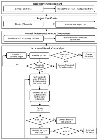
Figure 1.
Study framework.
Various definitions and applications of the term accessibility exist in the literature [66,67,68]. Therefore, the selection of accessibility measures depends on the accessibility-related problems that needs to be addressed [69,70]. Transportation-related accessibility measures are often developed using the distance traveled or the time it takes to reach destinations [71]. As the daily traffic volume in low-volume roads (LVRs) is very low (less than 400 vehicles) [72], it is not necessarily appropriate to prioritize and implement LVR projects based on such factors as traffic congestion as system performance measures because the LVR networks operate under capacity under normal conditions [1]. Therefore, this study uses the network-level travel time as the LVR network accessibility measure. Equation (1) shows the network accessibility metric used to determine the network accessibility performance of LVR networks due to the implementation of single or bundle LVR projects.
where NA = network accessibility; tij = travel time between nodes i and j in the network.
The benefit associated with a project or project bundle due to the change in network accessibility should be monetized to use the developed framework. However, it is very difficult to estimate the value of travel time. Hence, the unit travel time value is often established by transportation agencies [31]. These travel time values are updated using consumer price indices to take into account the time value of money. This study used the average values of travel time in the U.S. The average value of the unit travel time considering all vehicle classes (i.e., small automobiles, medium-sized automobiles, multiple classes of trucks) is used to demonstrate the developed framework. The unit travel time’s average value is calculated to be $18.9/h (in 2005 dollars). The unit travel time value is then converted into 2019 dollars using Equation (2).
where TTVx = travel time value in year x (in dollars); TTVy = travel time value in year y (in dollars); CPIx = consumer price index in year x; and CPIy = consumer price index in year y.
TTVx = TTVy ∗ (CPIx/CPIy)
The average consumer price indices for 2005 and 2019 were $195.30 and $254.95, respectively [73]. The value of the travel time calculated using Equation (2) is $24.67/h (in 2019 dollars).
Incremental benefit–cost analysis (IBCA) procedure can be used to compare various public projects [74], such as road infrastructure projects considered in this study. First, the total cost and the total benefit associated with each candidate project or project bundle is determined. Then, the benefit/cost ratio (BCR) of each candidate project or project bundle is calculated. If we suppose the BCR of a project or project bundle is less than 1.0, then the project or project bundle is eliminated from the analysis because the project is considered not worth implementing when compared to the do-nothing alternative. On the other hand, if the BCR ≥ 1.0, the candidate project or project bundle is considered in the further IBCA analysis.
Once all candidate projects and project bundles with BCR ≥ 1.0 are identified, the IBCA procedure requires ranking of candidate projects and project bundles based on their total project cost, beginning with the lowest cost. The ranking of projects based on their total cost is crucial in the IBCA procedure to conduct a pair-wise comparison between the lowest and the higher cost candidate projects. Additionally, it helps to check if the incremental cost due to the higher cost alternatives is justified based on the attained incremental benefit–cost value. The incremental costs and incremental benefits between the first and the second lower-cost candidate projects are calculated using Equations (3) and (4).
where ∆C = incremental cost (∆C) (in dollars); TC2 = the total cost of the second lower-cost candidate project (in dollars); TC1 = the total cost of the first lower-cost candidate project (in dollars); ∆B = incremental benefit (∆B) (in dollars); TB2 = the unit network-level benefit of the second lower-cost candidate project (in dollars); TB1 = the unit network-level benefit of the second lower-cost candidate project (in dollars). Then, the incremental benefit–cost ratio, , is determined. If , the first lower-cost candidate project is eliminated, and the second lower-cost project is considered for further pair-wise comparison. This procedure is repeated, for the remaining candidate projects. At the end of the IBCA procedure, only one candidate project (a single project or project bundle) comes out as a winner and is recommended for implementation. In general, the incremental benefit/cost analysis (IBCA) of mutually exclusive projects aims to select a project or a bundle of projects that maximize the IBCA value.
The network-level benefit due to a project or project bundle is computed using Equation (5).
where NLBX = the network-level benefit due to a project or project bundle x (in dollars); NABN = network accessibility of the base network (in hours); NAX = network accessibility due to implementation of a project or project bundle x (in hours); TTV = travel time value per hour ($/h). As explained above, the travel time value is calculated to be $24.67/h (in 2019 dollars).
NLBX = (NABN − NAX) ∗ TTV
After determning the the network accessibility values of the LVR networks using Equation (1), Equaton (6) is used to calculate the percent change in network accessibility (i.e., the benefits) due to each single or bundle LVR project.
where PNAx = percent change or the benefit in network accessibility due to an LVR project x; NABN = network accessibility of the base network; NAx = network accessibility of the network with LVR project x implemented.
3. Case Study
The developed framework was demonstrated using a low-volume road (LVR) network shown in Figure 2 [75]. The case study LVR network has 17 nodes and 24 links. The nodes may represent intersections, rural cities, distribution centers, etc., in the LVR network, depending on scope of the analysis. The numbers shown on each link represent the impedance of the link, measured by travel time in hours. The dotted lines in Figure 2 represent candidate LVR Projects A, B, C, and D with travel times (in hours) of 0.7, 1.4, 0.6, and 1.9, respectively.
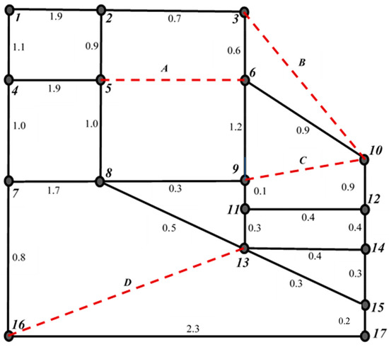
Figure 2.
Case study network [75].
The IBCA framework requires project costs as one of the inputs. The cost of constructing a new two-lane low-volume road (such as rural road) can vary between $2 million and $3 million per mile [76], representing cost variations that exist in real-world applications due to differences in highway classes that affect pavement design requirements, spatial locations, etc. [76]. Therefore, the IBCA framework is demonstrated, assuming that candidate projects will cost $2.5 million per mile. Table 1 shows the total project cost of the candidate LVR projects and project bundles. It is important to note that there exist other types of transportation costs associated with each project or project bundle that should be included in the IBCA procedure whenever data are available. These costs include agency costs, user costs, and community costs [31,77]. In this study, it is also assumed that the total cost of two or more projects is equal to the sum of the individual project costs due to lack of sufficient data. For example, as shown in Table 1, the cost of project bundle AB is equal to the sum of the costs of project A and B (i.e., $1.75 M + $2.5 M = $4.2 M). However, in real world situations, the cost of project bundles may be less than the sum of the individual projects forming the bundle due to existence of economies of scale [1]. Therefore, whenever data availability permits, it is useful to consider the impact of project bundling in the overall project cost in the IBCA framework.

Table 1.
Total project cost of LVR projects.
4. Results
4.1. Selection of the Best LVR Project
Table 2 shows the benefit–cost ratio (BCR) values of the single or bundle projects and the corresponding LVR network. These BCR values were used in the IBCA procedure shown in Table 3. Then, the best project or project bundle was selected among all individual LVR projects (i.e., projects A, B, C, or D) or their project bundles.
Table 2.
Benefit–cost ratio of LVR projects.
Table 3.
Pair-wise comparison of LVR networks.
Table 3 presents results of the pair-wise comparison of the LVR network developed considering the candidate LVR projects. The first row shows ranking of networks based on the total cost requirement of the candidate projects. For example, the total cost of Project C is the lowest among all single or bundle projects and hence was listed first. The first column lists pairs of networks to be compared and the second column shows the corresponding incremental benefit–cost ratio (BCR) ratio values. For example, the incremental BCR value when the network BN+C is compared with the do-nothing (DN) alternative is 746.9, which is greater than 1, implying that candidate Project C is preferred to the DN alternative. In Step 2, the next higher cost alternative, BN+A, is compared to BN+C, the winner of the pair-wise comparison in Step 1. In Step 2, the higher cost alternative, BN+A, is eliminated because the incremental BCR value is less than 1.0, implying that the additional investment cost due to candidate Project A cannot be justified. In all other steps, similar procedure of LVR network selection and elimination is followed. At the last step, Step 14, it is shown that the incremental BCR value is less than 1.0, indicating that the network BN+ACD is the best network among all networks in terms of maximizing network accessibility benefits. Therefore, the corresponding candidate Project Bundle ACD is selected for implementation.
The results shown in Table 3 generally show that it is not trivial to select the best candidate LVR project without applying the ICBA procedure. For example, one can expect that the simultaneous implementation of all the LVR projects (i.e., A, B, C, and D) could bring the highest network accessibility benefits. However, the results show that this is not necessarily the case because, as shown in Table 3, Project Bundle ACD is preferred to Project Bundle ABCD.
4.2. Disruption-Induced Change in Network Accessibility
In this study, the impact of network disruption events (such as flooding, earthquakes, traffic accidents, etc.) on the network accessibility of LVR networks was evaluated considering various network disruption scenarios. A Monte Carlo simulation program was written in Python [78] to simulate the network disruption events and identify network links or nodes likely to be affected by the network disruption event. Table 4 shows network disruption simulation results for BN+AC and BN+BCD networks considering two-link, four-link, and six-link disruption scenarios. For example, for Scenario 1 (i.e., the two-link disruption scenario), the disrupted links in the case of BN+AC network after 107 simulation cycles were links 13–16 and 8–13. The spatial locations the links is shown in Figure 2.
Table 4.
Network disruption simulation results.
Figure 3 shows the results of the percent change in network accessibility due to various link disruption scenarios. The results show that, as the number of disrupted links increases, there could be an increase in percent reduction in network accessibility. For example, in the case of the four-link disruption scenario, the percent reduction in network accessibility of the BN+AC network is 0.24%, whereas, in the case of a six-link disruption scenario, the network’s percent reduction in network accessibility is 0.30%. A similar observation can be made for the case of BN+BCD.
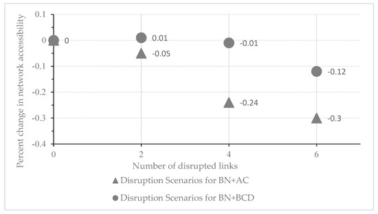
Figure 3.
Percent change in network accessibility considering link disruption scenarios.
The results also show that the implementation of more LVR projects could help minimize the percent reduction in network accessibility regardless of the number of link disruption. For example, considering a four-link disruption scenario, the BN+BCD’s percent reduction in network accessibility is only 0.01%, whereas that of BN+AC is 0.24%. A similar observation can be made for the cases of two-link and six-link disruption scenarios.
In some cases, the network accessibility could be improved after the occurrence of network disruption events. For example, the LVR network BN+BCD has shown a 0.01% increase in network accessibility after a two-link disruption event occurred, indicating that transportation decision-makers could consider LVR projects as one of the many options to mitigate the degradation in network accessibility due to network disruption events at planning stage.
4.3. Selection of LVR Projects Considering Network Disruption Scenarios
Table 5 shows selected LVR projects based on the IBCA procedure considering two-link, four-link, and six-link network disruption scenarios. As shown in the table, the best performing networks according to the IBCA procedure are BN+AD, BN+AC, and BN+ACD, respectively. Therefore, Project Bundles AD, AC, and ACD should be implemented in the case of two-link, four-link, and six-link disruption scenarios, respectively.
Table 5.
Results of prioritization of LVR projects based on the IBCA procedure and considering network disruption events.
These results indicate that the selection of LVR projects or project bundles may depend on the level of disruption events (i.e., how many links are expected to be disrupted based on the severity level of the disruption event). The results also show that project bundles containing LVR Project A are preferred for the three disruption scenarios considered in the study, implying that some LVR projects are very vital for maximizing LVR network resilience after the occurrence of network disruption events that degrade network accessibility performance regardless of the level of investment made in improving the network accessibility. The vitality of the LVR projects could be attributed to their spatial locations in the network that help improve accessibility by reducing the overall travel time required to travel among nodes (counties, cities, states, etc.) in the network.
It is interesting to see from results shown in Table 5 that the implementation of all the LVR projects (i.e., Project Bundle ABCD) may not be useful to maximize the LVR network performance based on the IBCA procedure. Therefore, transportation investment decision-makers should use the proposed IBCA procedure to identify those LVR projects that need not be implemented to maintain network accessibility after an expected network disruption scenario. That way, the decision-makers could reduce investment costs and ensure the availability of funds for future LVR network improvement to maximize network accessibility resilience in areas where disruption events often occur.
5. Discussion
The results of this study provide valuable information for transportation and infrastructure investment decision-makers that plan to maximize the LVR network accessibility by investing economically. By implementing the IBCA procedure, the decision-makers can identify which single or bundle projects should be implemented to improve the accessibility of the LVR network at network-level. Additionally, transportation investment decision-makers could avoid implementing a large number of projects (and hence saving investment costs) to achieve the same level of accessibility that could be attained by implementing a single or a small number of projects.
Network disruption scenarios could severely damage an LVR network, causing significant degradation in the accessibility of the LVR network. However, transportation investment decision-makers have options of developing mitigation strategies at planning stages by conducting network disruption scenarios and identifying a single or a bundle of LVR projects. That is, the decision-makers could ensure the LVR network’s resilience to degradation in accessibility level, and, in some cases, they could improve the accessibility level, depending on the contribution of the selected LVR project or project bundles to the network accessibility.
Previous studies did not develop a framework that incorporates the incremental accessibility benefits of higher-cost LVR projects in the project prioritization procedure. In addition, they did not extensively consider the impact of simultaneous implementation of multiple LVR projects on network accessibility benefits per unit cost of investment. This study could help researchers and decision-makers consider the IBCA procedure developed in this study and incorporate other parameters of interest when required.
The IBCA procedure developed in this study is especially beneficial currently because, as noted in [79], there are insufficient funds to implement infrastructure projects. This study’s findings generally indicate that extensive analysis of single and bundle LVR projects is essential to maximize network accessibility benefits and ensure sustainability of LVR network performance by effectively utilizing available infrastructure funds. A framework, such as the one developed in this study, is beneficial to serve this purpose.
Future research could expand the IBCA framework, considering other infrastructure-related costs such as user, community, and environmental costs (such as air pollution and noise pollution costs) to ensure the sustainability of infrastructure performance. Future research could also improve the IBCA framework by incorporating the concept of economies of scale related to candidate LVR projects to help realize the sustainability of infrastructure funding and maximize LVR network accessibility benefits. Future research could also utilize the IBCA procedure to evaluate LVR project selection outcomes with respect to network accessibility benefits per unit cost of investment at the post-implementation stage, the during-implementation stage (for example, when planning network-wide construction activities that force complete link closure), or the pre-implementation stage (i.e., at planning stage) of LVR projects.
6. Conclusions
The research results show that low-volume road (LVR) projects’ accessibility benefits depend on their relative spatial location in the network and their total project cost, suggesting the importance of the developed IBCA framework to capture such spatial effects and maximize the sustainability of LVR network performance. LVR projects are useful for ensuring the sustainability of network accessibility performance not only during normal operating conditions but also after the occurrence of network disruption events (such as flooding, earthquakes, etc.) that degrade the LVR network accessibility performance.
The IBCA framework is particularly useful for investment decision-makers to justify selecting a higher-cost project that may play a significant role in the degree of accessibility of an LVR network. The proposed framework helps to maximize the accessibility-related economic benefits of road infrastructure investments and ensure the sustainability of LVR network performance.
Funding
This research received no external funding.
Institutional Review Board Statement
This study did not involve humans or animals.
Informed Consent Statement
Not applicable.
Data Availability Statement
This study did not report any data.
Conflicts of Interest
The author declares no conflict of interest.
References
- Woldemariam, W. Goal Programming Framework for Prioritization of Low-Volume Road Projects Considering Network Accessibility and Stakeholders’ Preferences. Transp. Res. Rec. 2020. [Google Scholar] [CrossRef]
- Stępniak, M.; Rosik, P. The Role of Transport and Population Components in Change in Accessibility: The Influence of the Distance Decay Parameter. Netw. Spat. Econ. 2018, 18, 291–312. [Google Scholar] [CrossRef] [Green Version]
- Büttner, B.; Kinigadner, J.; Ji, C.; Wright, B.; Wulfhorst, G. The TUM Accessibility Atlas: Visualizing Spatial and Socioeconomic Disparities in Accessibility to Support Regional Land-Use and Transport Planning. Netw. Spat. Econ. 2018, 18, 385–414. [Google Scholar] [CrossRef] [Green Version]
- Garcia, C.S.H.F.; Macário, R.; de Araújo Girão Menezes, E.D.; Loureiro, C.F.G. Strategic Assessment of Lisbon’s Accessibility and Mobility Problems from an Equity Perspective. Netw. Spat. Econ. 2018, 18, 415–439. [Google Scholar] [CrossRef]
- Buchholz, S.; Gamst, M.; Pisinger, D. Finding a Portfolio of Near-Optimal Aggregated Solutions to Capacity Expansion Energy System Models. SN Oper. Res. Forum 2020, 1, 7. [Google Scholar] [CrossRef] [Green Version]
- An, M.; Casper, C. Integrating travel demand model and benefit-cost analysis for evaluation of new capacity highway projects. Transp. Res. Rec. 2011, 2244, 34–40. [Google Scholar] [CrossRef]
- Gurganus, C.F.; Gharaibeh, N.G. Project selection and prioritization of pavement preservation. Transp. Res. Rec. 2012, 2292, 36–44. [Google Scholar] [CrossRef]
- AASHTO. User Benefit Analysis for Highways; AASHTO: Washington, DC, USA, 2003. [Google Scholar]
- Christopher, R.B.; Ian, D.G. Modelling Road User and Environmental Effects in HDM-4, 7th ed.; HDM Global: Paris, France, 2001; Volume 7. [Google Scholar]
- Forkenbrock, J.; Weisbrod, E. Guidebook for Assessing the Social and Economic Effects of Transportation Projects; EBP: Washington, DC, USA, 2001. [Google Scholar]
- Gwilliam, K. The Value of Time in Economic Evaluation of Transport Projects–Lessons from Recent Research; TRB: Washington, DC, USA, 1997. [Google Scholar]
- Heggie, I. Transport. Engineering Economics; McGraw-Hill: New York, NY, USA, 1972. [Google Scholar]
- OPUS International Consultants. Review of VOC-Pavement Roughness Relationships Contained in Transfund’s Project Evaluation Manual; OPUS International Consultants: Lower Hutt, New Zealand, 1999. [Google Scholar]
- Stopher, P.; Meyburg, A. Transportation Systems Evaluation; Lexington Books, D.C. Health and Company: Lexington, TX, USA, 1976. [Google Scholar]
- Wardman, M. The value of travel time a review of british evidence. J. Transp. Econ. Policy 1998, 32, 285–316. [Google Scholar]
- Zaniewski, J. Vehicle Operating Costs, Fuel Consumption, and Pavement Type and Condition Factors; TRB: Washington, DC, USA, 1982. [Google Scholar]
- NYSDOT. Vulnerability Manuals for Bridge Safety Assurance Program; NYSDOT: New York, NY, USA, 2002.
- Canter, W. Environmental Impact Assessment; McGraw-Hill: New York, NY, USA, 1995. [Google Scholar]
- Cohn, F.; McVoy, R. Environmental Analysis of Transportation Systems; Wiley: New York, NY, USA, 1982. [Google Scholar]
- Faiz, A.; Weaver, C.S.; Walsh, M.P. Air pollution from motor vehicles (Standards and Technologies for Controlling Emissions); World Bank Publications: Washington, DC, USA, 1996. [Google Scholar] [CrossRef] [Green Version]
- FTA. Transit Noise and Vibration Impact Assessment; FTA: Washington, DC, USA, 1995.
- Ortolano, L. Environmental Regulation and Impact Assessment; Wiley: New York, NY, USA, 2001. [Google Scholar]
- Sinha, K.; Teleki, G.; Alleman, J.; Cohn, L.; Radwan, E.; Gupta, A. Environmental Assessment of Land Transport Construction and Maintenance; Prepared for the Infrastructure and Urban Development Department, World Bank: Washington, DC, USA, 1991. [Google Scholar]
- USDOT. FHWA Traffic Noise Model® User’s Guide; USDOT: Washington, DC, USA, 2004.
- USEPA. User’s Guide to MOBILE6.0 Mobile Source Emission Factor Model; USEPA: Washington, DC, USA, 2002.
- Cambridge Systematics. A Guidebook for Performance-Based Transportation Planning; Cambridge Systematics: Washington, DC, USA, 2000. [Google Scholar]
- NHI. Estimating the Impacts of Transportation Alternatives; NHI: Washington, DC, USA, 1995.
- OECD. Performance Indicators for the Road Sector, Organization for Economic Cooperation and Development; OECD: Paris, France, 2001. [Google Scholar]
- Pickrell, S.; Neumann, L. Linking performance masures with decision-making. In Proceedings of the National Academy of Sciences, 79th Annual Meeting of the Transportation Research Board, Washington, DC, USA, 9–13 January 2000. [Google Scholar]
- Poister, H. Strategic Planning and Decision Making in State Departments of Transportation; National Academies of Sciences, Engineering, and Medicine: Washington, DC, USA, 2004. [Google Scholar]
- Sinha, K.; Labi, S. Transportation Decision Making: Principles of Project Evaluation and Programming; John Wiley & Sons, Inc.: Hoboken, NJ, USA, 2007. [Google Scholar]
- Turner, S.; Best, M.; Shrank, D. Measures of Effectiveness for Major Investment Studies; TRB: College Station, TX, USA, 1996. [Google Scholar]
- Chandran, S.; Isaac, K.P.; Veeraragavan, A. Prioritization of Low-Volume Pavement Sections for Maintenance by Using Fuzzy Logic. Transp. Res. Rec. J. Transp. Res. Board 2007, 1989, 53–60. [Google Scholar] [CrossRef]
- Gokey, J.; Klein, N.; Mackey, C.; Santos, J.; Pillutla, A.; Tucker, S. Development of a prioritization methodology for maintaining Virginia’s bridge infrastructure systems. In Proceedings of the 2009 IEEE Systems and Information Engineering Design Symposium, SIEDS ’09, Charlottesville, VT, USA, 24 April 2009. [Google Scholar]
- Straehl, S.; Schintler, L. Montana Secondary Program Reform and Application of Goals Achievement Methodology to Project Prioritization. Transp. Res. Rec. 2004, 1895, 85–93. [Google Scholar] [CrossRef]
- Faiz, A. The promise of rural roads: Review of the role of low-volume roads in rural connectivity, poverty reduction, crisis management, and livability. Transp. Res. Rec. 2012. [Google Scholar] [CrossRef]
- Guerre, J.A.; Evans, J. Applying system-level performance measures and targets in the Detroit, Michigan, metropolitan planning process. Transp. Res. Rec. 2009, 2119, 27–35. [Google Scholar] [CrossRef]
- Akan, G.; Brich, S. Transportation project programming process for an urban area. Transp. Res. Rec. 1996, 1518, 42–47. [Google Scholar] [CrossRef]
- Galvan, G.; Agarwal, J. Community detection in action: Identification of critical elements in infrastructure networks. J. Infrastruct. Syst. 2018, 24, 04017046. [Google Scholar] [CrossRef] [Green Version]
- Bell, M.G.H. A game theory approach to measuring the performance reliability of transport networks. Transp. Res. Part B Methodol. 2000, 34, 533–545. [Google Scholar] [CrossRef]
- Karlaftis, M.; Kepaptsoglou, K. Performance Measurement in the Road Sector: A Cross-Country Review of Experience; International Transport Forum: Paris, France, 2012. [Google Scholar]
- Novak, D.C.; Sullivan, J.L.; Scott, D.M. A network-based approach for evaluating and ranking transportation roadway projects. Appl. Geogr. 2012, 34, 498–506. [Google Scholar] [CrossRef]
- Sullivan, J.L.; Novak, D.C.; Aultman-Hall, L.; Scott, D.M. Identifying critical road segments and measuring system-wide robustness in transportation networks with isolating links: A link-based capacity-reduction approach. Transp. Res. Part A Policy Pract. 2010, 44, 323–336. [Google Scholar] [CrossRef]
- Scott, D.M.; Novak, D.C.; Aultman-Hall, L.; Guo, F. Network robustness index: A new method for identifying critical links and evaluating the performance of transportation networks. J. Transp. Geogr. 2006, 14, 215–227. [Google Scholar] [CrossRef]
- Ismaeel, M.; Zayed, T. Integrated Performance Assessment Model for Water Networks. J. Infrastruct. Syst. 2018, 24, 04018005. [Google Scholar] [CrossRef]
- Adarkwa, O.; Attoh-Okine, N.; Schumacher, T. Using tensor factorization to predict network-level performance of bridges. J. Infrastruct. Syst. 2017, 23, 04016044. [Google Scholar] [CrossRef]
- Mouter, N. Dutch politicians’ use of cost–benefit analysis. Transportation 2017, 44, 1127–1145. [Google Scholar] [CrossRef] [Green Version]
- Roxas, N.R.; Fillone, A.M. Establishing value of time for the inter-island passenger transport of the Western Visayas region, Philippines. Transportation 2016, 43, 661–676. [Google Scholar] [CrossRef]
- Mizusawa, D.; McNeil, S. Generic methodology for evaluating net benefit of asset management system implementation. J. Infrastruct. Syst. 2009, 15, 232–240. [Google Scholar] [CrossRef]
- Szimba, E.; Rothengatter, W. Spending scarce funds more efficiently-including the pattern of interdependence in cost-benefit analysis. J. Infrastruct. Syst. 2012, 18, 242–251. [Google Scholar] [CrossRef]
- Zhao, L.; Chien, S.; Meegoda, J.; Luo, Z.; Liu, X. Cost-benefit analysis and microclimate-based optimization of a RWIS network. J. Infrastruct. Syst. 2016, 22, 04015021. [Google Scholar] [CrossRef]
- Godinho, P.; Dias, J. Cost-benefit analysis and the optimal timing of road infrastructures. J. Infrastruct. Syst. 2012, 18, 261–269. [Google Scholar] [CrossRef] [Green Version]
- Gregory, R.; Kangari, R. Cost/Benefits of Robotics in Infrastructure and Environmental Renewal. J. Infrastruct. Syst. 2000, 6, 33–40. [Google Scholar] [CrossRef]
- Li, Z.; Madanu, S. Highway Project Level Life-Cycle Benefit/Cost Analysis under Certainty, Risk, and Uncertainty: Methodology with Case Study. J. Transp. Eng. 2009, 135, 516–526. [Google Scholar] [CrossRef]
- Labi, S.; Sinha, K.C. Life-cycle evaluation of flexible pavement preventive maintenance. J. Transp. Eng. 2005, 131, 744–751. [Google Scholar] [CrossRef]
- Odeck, J.; Kjerkreit, A. The accuracy of benefit-cost analyses (BCAs) in transportation: An ex-post evaluation of road projects. Transp. Res. Part A Policy Pract. 2019, 120, 277–294. [Google Scholar] [CrossRef]
- Manzo, S.; Salling, K.B. Integrating Life-cycle Assessment into Transport Cost-benefit Analysis. In Proceedings of the Transportation Research Procedia, Amsterdam, The Netherlands, 27 June 2016. [Google Scholar]
- Batarce, M.; Muñoz, J.C.; Ortúzar, J.D.D. Valuing crowding in public transport: Implications for cost-benefit analysis. Transp. Res. Part A Policy Pract. 2016, 91, 358–378. [Google Scholar] [CrossRef]
- Ito, Y.; Managi, S. The potential of alternative fuel vehicles: A cost-benefit analysis. Res. Transp. Econ. 2015, 50, 39–50. [Google Scholar] [CrossRef] [Green Version]
- Yen, K.S.; Lasky, T.A.; Ravani, B. Cost-benefit analysis of mobile terrestrial laser scanning applications for highway infrastructure. J. Infrastruct. Syst. 2014, 20, 04014022. [Google Scholar] [CrossRef]
- Ikpe, E.; Hammon, F.; Oloke, D. Cost-benefit analysis for accident prevention in construction projects. J. Constr. Eng. Manag. 2012, 138, 991–998. [Google Scholar] [CrossRef]
- Myers, L.; Najafi, F. Performance bond benefit-cost analysis. Transp. Res. Rec. 2011, 2228, 3–10. [Google Scholar] [CrossRef]
- Berechman, J.; Paaswell, R.E. Evaluation, prioritization and selection of transportation investment projects in New York City. Transportation 2005, 32, 223–249. [Google Scholar] [CrossRef]
- Proost, S.; Dunkerley, F.; Van der Loo, S.; Adler, N.; Bröcker, J.; Korzhenevych, A. Do the selected Trans European transport investments pass the cost benefit test? Transportation 2014, 41, 107–132. [Google Scholar] [CrossRef] [Green Version]
- West, J.; Börjesson, M. The Gothenburg congestion charges: Cost–benefit analysis and distribution effects. Transportation 2018, 47, 145–174. [Google Scholar] [CrossRef] [Green Version]
- Geurs, K.T.; van Wee, B. Accessibility evaluation of land-use and transport strategies: Review and research directions. J. Transp. Geogr. 2004, 12, 127–140. [Google Scholar] [CrossRef]
- Beria, P.; Debernardi, A.; Ferrara, E. Measuring the long-distance accessibility of Italian cities. J. Transp. Geogr. 2017, 62, 66–69. [Google Scholar] [CrossRef]
- Morris, J.M.; Dumble, P.L.; Wigan, M.R. Accessibility indicators for transport planning. Transp. Res. Part A Gen. 1979, 13, 91–109. [Google Scholar] [CrossRef]
- Martín, J.C.; Reggiani, A. Recent methodological developments to measure spatial interaction: Synthetic accessibility indices applied to high-speed train investments. Transp. Rev. 2007, 27, 551–571. [Google Scholar] [CrossRef]
- Vandenbulcke, G.; Steenberghen, T.; Thomas, I. Mapping accessibility in Belgium: A tool for land-use and transport planning? J. Transp. Geogr. 2009, 17, 39–53. [Google Scholar] [CrossRef]
- Páez, A.; Scott, D.M.; Morency, C. Measuring accessibility: Positive and normative implementations of various accessibility indicators. J. Transp. Geogr. 2012, 25, 141–153. [Google Scholar] [CrossRef]
- FHWA. Manual on Uniform Traffic Control Devices for Streets and Highways. Available online: https://mutcd.fhwa.dot.gov/ (accessed on 28 August 2020).
- BLS. Consumer Price Index. Available online: https://www.bls.gov/regions/midwest/data/consumerpriceindexhistorical_us_table.pdf%0D (accessed on 2 January 2020).
- Blank, L.; Tarquin, A. Engineering Economy, 8th ed.; McGraw-Hill Education: New York, NY, USA, 2018. [Google Scholar]
- Woldemariam, W.; Labi, S.; Faiz, A. Topological Connectivity Criteria for Low-Volume Road Network Design and Improvement. In Proceedings of the 12th International Conference on Low-Volume Roads, Kalispell, MT, USA, 15–18 September 2019; Transportation Research Board: Kalispell, MT, USA, 2019; pp. 150–167. [Google Scholar]
- ARTBA. Frequently Asked Questions. Available online: https://www.artba.org/about/faq/ (accessed on 15 December 2019).
- Woldemariam, W.; Murillo-Hoyos, J.; Labi, S. Estimating annual maintenance expenditures for infrastructure: Artificial neural network approach. J. Infrastruct. Syst. 2016, 22, 04015025. [Google Scholar] [CrossRef]
- Van Rossum, G. The Python Language Reference; Network Theory Ltd.: Amsterdam, The Netherlands, 2012. [Google Scholar]
- Woldemariam, W. A framework for transportation infrastructure cost prediction: A support vector regression approach. Transp. Lett. 2021, 1–7. [Google Scholar] [CrossRef]
Publisher’s Note: MDPI stays neutral with regard to jurisdictional claims in published maps and institutional affiliations. |
© 2021 by the author. Licensee MDPI, Basel, Switzerland. This article is an open access article distributed under the terms and conditions of the Creative Commons Attribution (CC BY) license (https://creativecommons.org/licenses/by/4.0/).