Article

Innovativeness, Work Flexibility, and Place Characteristics: A Spatial Econometric and Machine Learning Approach

by
Mehmet Güney Celbiş
1,2,*,†,
Pui-Hang Wong
2,3,†,
Karima Kourtit
4,5,6,† and
Peter Nijkamp
4,5,6,†
1
Department of Economics, Yeditepe University, Istanbul 34755, Turkey
2
United Nations University-Maastricht Economic and Social Research Institute on Innovation and Technology (UNU-MERIT), 6211 Maastricht, The Netherlands
3
Maastricht Graduate School of Governance, School of Business and Economics, Maastricht University, 6211 Maastricht, The Netherlands
4
Faculty of Management, Open University, 6419 Heerlen, The Netherlands
5
Centre for European Studies, Alexandru Ioan Cuza University, 700506 Iași, Romania
6
School of Architecture, Planning and Design, Polytechnic University, Ben Guerir 43150, Morocco
*
Author to whom correspondence should be addressed.
These authors contributed equally to this work.
Sustainability 2021, 13(23), 13426; https://doi.org/10.3390/su132313426
Submission received: 31 October 2021 / Revised: 15 November 2021 / Accepted: 24 November 2021 / Published: 3 December 2021

Abstract

:
This paper seeks to study work-related and geographical conditions under which innovativeness is stimulated through the analysis of individual and regional data dating from just prior to the smartphone age. As a result, by using the ISSP 2005 Work Orientations Survey, we are able to examine the role of work flexibility, among other work-related conditions, in a relatively more traditional context that mostly excludes modern, smartphone-driven, remote-working practices. Our study confirms that individual freedom in the work place, flexible work hours, job security, living in suburban areas, low stress, private business activity, and the ability to take free time off work are important drivers of innovation. In particular, through a spatial econometric model, we identified an optimum level for weekly work time of about 36 h, which is supported by our findings from tree-based ensemble models. The originality of the present study is particularly due to its examination of innovative output rather than general productivity through the integration of person-level data on individual work conditions, in addition to its novel methodological approach which combines machine learning and spatial econometric findings.
JEL Classification:
J08; J22; O30; O31; C40

1. Introduction

There is a great amount of strong empirical evidence for the existence of a relationship between innovation and economic growth. However, this relationship seems to depend on complex socioeconomic attributes, particularly in the context of regional economies [1,2]. Innovation itself, for its part, is the result of sophisticated interactions of social, economic, historical, and, not least of all, individual factors. Unequivocally, innovation is triggered and inspired via ideas developed by individuals, and the development of such ideas is subject to individual creativity.
A significant amount of empirical evidence indicates that the systems approach successfully explains the variations in innovation performance across locations and time periods (e.g., [3,4]). However, the focus on multiple actors and purposeful interactions tends to downplay the role of individuals and the “randomness” of innovative activities. Several studies have observed that innovative behaviour is induced by individuals’ original ideas, and the road towards innovation performance and success is often shaped by individual creativity (e.g., [5,6,7]). Indeed, many patents are owned by individual inventors [8]. Furthermore, original ideas that result in innovative products or know-how are sometimes spontaneous and often originate from non-R&D-related activities outside firms [9,10,11,12].
In common, previous studies invariously adopt a human-resource approach and use firm-level data to investigate the work–innovation nexus. By contrast, this paper looks at work–innovation linkage from the perspective of individuals. On the basis of these observations, this study addresses the following questions: Which factors shape or determine creativeness? Is creativeness a product of the human mind determined by neural brain activity, or is the work and living environment of an individual a facilitating factor for creative ideas? In order to answer these questions, the present study will zoom in on the individual’s work environment, as well as on regional factors that are likely to influence a person’s creativity (see also [13]). In performing this study, we focus on the 2005–2006 period, which is just before the introduction of modern smartphones followed by tablets, which brought considerable remote and flexible working practices for many individuals [14,15]. While devices that can be defined as smartphones already existed by the period analyzed in this study, the arguably faster and efficient devices alongside with software such as the Apple iOS and the Google Android operating system had yet been introduced to global markets [14,16]. These technologies have enabled individuals to connect and engage in their work outside of the employer’s locations at any time of the day, resulting in increased flexibility and organization of work hours [17,18]. As a result, the importance of location and the spatial dimension of inequalities in the accessibility of communication infrastructures with regard to regional industries, including the education sector, has become even more pronounced [19,20]. This newly induced type of flexibility may be involuntary or voluntary, even resulting in behaviors such as compulsive and continuous monitoring of work-related emails and blurring the borders between work and leisure times [16,17]. On the other hand, through our focus on a modern but pre-widespread smartphone use period, we are able to study the roles of job flexibility in a relatively more traditional sense without being subject to confounding elements arising from the prevalent usage of smartphones and tablets. In other words, job flexibility as measured in this study mostly captures “true” flexibility, rather than a type of flexibility caused by the voluntary or involuntary out-of-work habits. Consequently, using survey data from 18 European countries, this study examines the role of both individual work conditions and other place-based factors that influence regional innovation activities. The results from our analysis show that work-leisure balance and geographical attributes pertaining to city life and industrial clusters can significantly predict the innovation performance of a region. This result also holds after controlling for spatial spillovers and applying machine learning algorithms as an alternative methodological approach. In short, we find that flexible work time, job security, and job autonomy are conducive to regional innovation performances. Given our focus on regional innovation, this study provides additional evidence on the work–innovation linkage which hitherto has been mostly restricted to the firm level. As the RIS approach and the recent open innovation literature suggest, innovation often occurs in non-firm settings and involves actors outside the industry [21,22,23]. Our study addresses this gap and generalizes these insights at a regional level.
This study contributes to the area of innovation studies and the related human resources management HRM literature in three ways. Firstly, we adopt a workers’ perspective in order to analyse the impact of work-related factors on innovation at the regional level. While there is a burgeoning literature on the impact of HRM practices on innovation performance (see Laursen et al. [24] for a survey of the literature), many studies adopt the firm’s perspective and use firm-level data to understand the mechanisms underlying individual creativity and innovation performance. However, the use of this type of data limits the scope to only innovative activities that take place at the firm level. For example, regarding flexible working time, Arvanitis [25] finds that a higher level of individual work-time flexibility has a positive and statistically significant impact on innovation propensity and innovation success. Similarly, a study by Burtch et al. [26] suggests that the positive effects on innovation can be explained by the fact that HRM practices allow workers to redeploy resources strategically, thus stimulating innovative activities. Nevertheless, Arvanitis et al. [27] found that the impact of flexible work time is usually very small.
Secondly, this study integrates management innovation into the regional innovation systems RIS framework. Birkinshaw et al. [28] defined management innovation as a new management practice that furthers organisational goals. While this paper posits and finds that flexible work hours and a relaxing work environment are conducive to innovation, we also maintain that place-based factors underlying the RIS approach are also necessary to activate the HRM–innovation linkage. While workers may generate original ideas, the intellectual capital and knowledge base of a region, its university–industry linkage, its culture of idea sharing and cooperation, the rules that govern knowledge flow, and other factors that underlie the RIS approach are crucial in the process of turning a new idea into a patent or a new product. For instance, Kianto et al. [29] show that intellectual capital mediates the effect of knowledge-based HRM policies (e.g., concerning recruitment, training, and appraisal system) on innovation performance. As such, this study places the emerging literature on work–innovation linkage back in the context of RIS and enriches the RIS approach by adding a new layer to the systems tradition.
Finally, this study employs both spatial econometrics and machine learning (ML) techniques in the analysis. Machine learning techniques have increasingly been used in innovation studies. For example, Suominen et al. [30] used Latent Dirichlet Allocation (LDA) to show the evolution of the knowledge profiles of firms in the telecommunication industry. Ballestar et al. [31] applied Automated Nested Longitudinal Clustering (ANLC) and neural networks to evaluate the effect of a new employment policy on the productivity of university researchers in Madrid. Recently, Kim and Sohn [32] used semantic analysis to identify convergence patterns of new technology from patent data. However, to the best of our knowledge, this is the first study to complement findings from spatial econometrics with various machine learning analyses in order to study RIS and management innovation.
The remainder of the article is organized as follows. Section 2 outlines the influential contributions to the literature. Section 3 outlines the theoretical framework and provides the foundation for our econometric model. Next, Section 4 describes the data and visualizes the statistical distributions of key variables. Section 5 summarizes the findings from econometric estimations that serve as a reference for our machine learning techniques. These techniques are outlined in Section 6, which also presents several findings that are not covered by the preceding econometric analyses. Section 7 makes concluding remarks.

2. Literature Review

Ever since the seminal writings of Schumpeter [33], the theme of innovation has been high on the agenda of both the research community and decision makers in the public and private sectors. Numerous empirical studies have shown that innovation results in economic progress, while innovation itself is influenced by an array of factors and relations (see for instance [34,35]). The National Innovation Systems (NIS) and the RIS approaches describe innovation as an activity undertaken by a network of actors subject to an institutional environment [36,37]. The systems approach highlights the importance of interactions (e.g., learning, knowledge flow, and policies) among a network of actors such as universities, industries, and national or regional governments [38]. The differences between these interactive activities and institutions, which include, but are not limited to, financial capacity, organisational structure, social capital, and culture, determine the differences in innovation performance and economic growth across regions [39].
Although the topic of work–innovation nexus is relatively new in innovation studies, the role of individual creativity on innovation in professional work environments has been studied in the field of HRM. In an early study, Amabile et al. [40] argued that the social environment is likely to affect individual creativity and, therefore, influences the innovative output of an organization and its members. This social environment is characterized by five conceptual categories of work-related factors: an organizational culture that encourages risk-taking and creative attitudes; job autonomy that cultivates a sense of ownership and responsibility; the availability of sufficient resources; and stress from workload pressures and organizational impediments such as conservatism that limits and discourages personal creativity. More recent studies, however, have found only mixed evidence about the importance of these factors (see below).
A concept that is closely related to job flexibility is job autonomy. In this regard, Laursen et al. [41] and, more recently, Krammer [42] showed that employees’ greater job autonomy contributes to the innovative performance of a firm (also see the literature review by Seeck and Diehl [43] on this relationship). Along similar lines, Arvanitis [25] found that greater decision-making power and span of control have positive impacts on both product and process innovation. Nevertheless, based on interviews with the executives of 49 technology small and medium-sized enterprises (SMEs) in Germany, Strobel et al. [44] reported that setting unclear tasks impedes innovative activity. As tasks related to innovation are not always well defined and require a high degree of cooperation, greater job autonomy could be harmful to innovation. In other words, the effects of task autonomy, flexible work hours, and job security on innovation remain unclear and more evidence is required. The present study contributes to the debate by providing additional confirmative evidence on the role of HRM practices.
Together with flexibility and autonomy, it has also been suggested that the level of security of an individual’s job is also related to innovative performance. Michie et al. [45] found that labour market deregulation (e.g., increasing use of short-term or temporary contracts) has been detrimental to innovation in the UK. A more detailed examination by Zhou et al. [46] suggests that firms with high shares of workers on fixed-term contracts usually perform well regarding imitative new products but poorly in relation to innovative new products. More recently, Hoxa and Kleinknecht [47,48] has shown that greater job insecurity is associated with poorer innovation performance in German firms. On the contrary, evidence observed by Arvanitis [25] indicates that firms that offer low job security are likely to have more product innovations. Drawing on these views and findings, we formulate (in Section 3) a theoretical framework that is both based on the synthesis of previous research on innovation, creativity, and personal autonomy.

3. Theoretical Background

As has been stipulated several times in the literature, “innovation is not manna from heaven” [49], but it is a product of knowledge-based human activity. In other words, we may hypothesize a relationship that explains how cognitive-oriented innovative performance is determined by various background factors (such as work stress, work effort, job cooperation, etc.). Celbis and Turkeli had shown that at the country level, innovation exhibits diminishing returns on work hours [50]. A similar relationship between leisure time and productivity in general is observed by Cui et al. [51]. We also assume that innovative performance does not increase linearly with respect to the number of work hours, but that there is some sort of inverted U-shape relationship. Consequently, we would have to look for the optimal work effort that maximizes innovativeness. We introduce this work-time related factor in the econometric specification of a knowledge production function, based on the seminal work by Jones [52]. We estimate the model in Section 5 alongside other variables that represent the degree of work-hours flexibility, freedom to organize one’s own work, ability to take time off, job security, and other personal and regional attributes that are explained later in this section.
We assume that all individuals, regardless of industry class and education level, can be creative idea-seekers if they are given the opportunity. Nevertheless, the generation of new knowledge by idea seekers in a region also depends on the existing stock of knowledge, which is not only specific to that region but exists in the country (or in the world) as a whole. We augment knowledge production function in two ways. Firstly, we introduce a set of individual level work-related factors and relevant regional characteristics. Secondly, as we assume that innovativeness may exhibit diminishing returns on work hours, we introduce a quadratic specification, followed by an alternative specification that considers a “deviation from the ideal work hours” effect. In other words, we assume that there exists an ideal length of work time that allows the idea seekers to work at their full potential, thus maximising regional innovativeness on average. When a region deviates from this optimum length of work time (either positively or negatively), its innovativeness will decay, and this decay increases exponentially.
Of course, the length of work time alone is not sufficient for understanding the conditions that shape a work-life balance that may be related to intellectual output. In order to account for time outside of work hours, apart from simply the length of work time, we also include, in our analysis, variables representing job flexibility (Flexible), freedom to organise daily work (Free), and ability to take time off (TimeOff).
The amount of stress to which individuals are subject may also have an impact on their creativity [53]. Furthermore, individuals may face stress resulting from low income, unemployment, and lack of job security. Therefore, it is plausible to include also additional explanatory variables (NeverStress, SomeStress, LowIncome, Unemployed, and NotSecure) that represent these attributes, as defined in Table 1.
In addition to factors related to work hours, some location-specific characteristics of the areas (regions and urban areas) where individuals reside may also be potential determinants of personal innovativeness. In a recent OECD report, it was shown that productivity is particularly driven by second-tier cities compared to core cities [54]. Furthermore, regional productivity in general is subject to local market access and agglomeration levels [55,56]. The International Social Survey Programme (ISSP) Work Orientations Survey (ISSP, 2005) provides classifications of the regions, i.e., areas, in which the respondents reside, and we accordingly distinguished the types of urban areas in our analysis, viz., large urban areas (BigUrb) and suburban areas (SubUrb) versus the reference category that consists of smaller settlements.
Past research has shown that entrepreneurship and human capital are key determinants of innovative activity and crucial factors of development in lagging areas [57,58,59,60]. Together with human capital, measured by the level of education (Degree), we include variables that measure the importance of entrepreneurs (Self) and of private industry (Private) within the model. In conjunction with industry characteristics, research and development (R&D) activities are proxied by the share of individuals in science-related professions (Science) and the health industry (Health).
We note here that the nexus of knowledge-based creativity and the determinants of individual and contextual factors may call for complementary model adjustments, depending on data availability. It may, therefore, be necessary to pursue further empirical alterations to the conceptual model sketched in this section before it can be used for estimation in our econometric models and for prediction in our machine learning models. Furthermore, innovative activities are not constrained by country or regional borders and usually involve international collaboration. In order to account for knowledge spillovers across borders, a consideration of spatial dependence will, thus, be pertinent. These issues are addressed in more detail in Section 5.
Table 1. Variable definitions.
NameDescriptionReference Category
P a t C a p Regional patent applications per million inhabitants in 2006. Source: Eurostat.
H o u r s Average hours worked per week by the respondents. Source: ISSP 2005-Work Orientations III.
F l e x i b l e Share of respondents who are either completely free to decide the start and end times of their work or who have some freedom to decide within certain limits.Share of respondents whose starting and finishing times are decided by the employer. Source: ISSP 2005-Work Orientations III.
F r e e Share of respondents who have complete or some freedom to organise their daily work.Share of respondents who have no freedom to organise their daily work. Source: ISSP 2005-Work Orientations III.
N o t S e c u r e Share of respondents who either disagree or strongly disagree that their job is secure.Share of respondents who either agree, strongly agree, or neither agree or disagree that their job is secure. Source: ISSP 2005-Work Orientations III.
N e v e r S t r e s s Share of respondents who state that their work is “never” or “hardly ever” stressful.Share of respondents who state that their work is “always” or “often” stressful (same reference dummy as the variable SomeStress). Source: ISSP 2005-Work Orientations III.
S o m e S t r e s s Share of respondents who state that their work is “sometimes” stressful.Share of respondents who state that their work is “always” or “often” stressful (same reference dummy as the variable NeverStress). Source: ISSP 2005-Work Orientations III.
S c i e n c e The share of respondents whose occupations belong to the category “physical, mathematical and engineering science professionals” listed under the International Standard Classification of Occupations 1988 (ISCO-88) as used in ISSP 2005.Share of respondents in all other occupations. Source: ISSP 2005-Work Orientations III.
P r i v a t e Share of respondents who work for private, non-public, or non-government firms.Share of respondents who work for the government or publicly owned firms (same reference dummy with the variable Self). Source: ISSP 2005-Work Orientations III.
S e l f Share of respondents who are self-employed.Share of respondents who work for the government or publicly owned firms (same reference dummy as the variable Private). Source: ISSP 2005-Work Orientations III.
D e g r e e Share of respondents who have completed at least a university degree.Share of respondents with education levels less than a university degree. Source: ISSP 2005-Work Orientations III.
U n e m p l o y e d Share of respondents who are unemployed.The share of respondents who have another employment status. Source: ISSP 2005-Work Orientations III.
L o w I n c o m e Share of respondents who either disagree or strongly disagree that their income is high.Share of respondents who either agree, strongly agree, or neither agree or disagree that their income is high. Source: ISSP 2005-Work Orientations III.
B i g U r b Share of respondents who live in an urbanised area/big city.Share of respondents who live in either a town or small city, country village, or farm or home in the country (same reference dummy as the variable SuBurb). Source: ISSP 2005-Work Orientations III.
S u b U r b Share of respondents who live in a suburban area or on the outskirts of a big city.Share of respondents who live in either a town or small city, country village, or farm or home in the country (same reference dummy as the variable BigUrb). Source: ISSP 2005-Work Orientations III.
T i m e O f f Share of respondents who state that taking time off during work hours is either “not too difficult” or “not difficult at all”.Share of respondents who state that taking time off during work hours is either “very difficult” or “somewhat difficult”. Source: ISSP 2005-Work Orientations III.
H e a l t h The share of respondents who belong to the occupations under the category “life science and health professionals” (excluding “nursing and midwifery professionals”) listed under the International Standard Classification of Occupations 1988 (ISCO-88) as used in ISSP 2005.Share of respondents in all other occupations. Source: ISSP 2005-Work Orientations III.
Note: Some variable definitions in this table may be partly or fully identical to those in ISSP 2005-Work Orientations III Codebook [61].

4. Data and Descriptive Statistics

Since, to the best of our knowledge, there are no studies that systematically investigate the relationship between individual work conditions and innovative activities at the regional level, there is no database that contains sufficient information on both variables. For our analysis, this limitation has necessitated the merging and aggregation of data from different sources. We obtained the data for the dependent variable from Eurostat, while all remaining data on the explanatory variables are taken from the International Social Survey Programme [61].
Challenges related to the compatibility of heterogeneous databases have influenced a number of our decisions regarding the design of research, as detailed later in this section, particularly those concerning the choice of the units of analysis and the measure of innovativeness.
The Work Orientations module III of the ISSP provides a number of interesting variables that allow us to test our hypotheses. The main advantage is that the survey asked about individuals’ attitudes towards work, work conditions, and employment arrangements. Table 1 presents the set of variables that we obtained from the ISSP survey and their descriptions, together with the reference categories that apply to certain variables. The descriptive statistics for each of these variables are displayed in Table 2.
The ISSP 2005 survey included 32 countries, 19 of them being in Europe. Unfortunately, as the regional classification in the ISSP is not always consistent with the Nomenclature of Territorial Units for Statistics (NUTS) classification of Eurostat, we have not been able to merge data for Norway. Therefore, the analysis comprises 18 European countries: Belgium, Bulgaria, Cyprus, Czechia, Denmark, Finland, France, Germany, Hungary, Ireland, Latvia, the Netherlands, Portugal, Slovenia, Spain, Sweden, Switzerland, and the United Kingdom. Due to similar compatibility issues, we had to regroup some of the regions based on the NUTS classification.
Measuring innovative activities is another major empirical challenge, and there is a lack of consensus in the literature on how this can be achieved. In our study, we have considered R&D expenditures, but the data points are missing for many of the regions. The Regional Innovation Scoreboard (RIS) provides an alternative. However, the data for the year 2006 are not available in the RIS. As a result, following Buesa et al. [62] and Bergamini et al. [63], we used patent applications as a proxy for regional innovativeness. The data for patent applications originate from Eurostat and are included in our analysis in per capita terms so as to adjust for scale effects. As a result, the dependent variable used in the present study (patents per capita) has 264 observations. When the 16 explanatory variables are included, the dataset attains 253 complete rows. The definition of all variables and their summary statistics are included, respectively, in Table 1 and Table 2.
In principle, one could use the number of patents that an individual applies for as a proxy of innovation, but owing to privacy issues, in general, it is not possible to obtain information related to the inventors’ time use and work flexibility. Therefore, prior to constructing econometric and machine learning models, we had to use regions instead of individuals as the units of analysis. This required us to aggregate (or average) our indicators for work conditions and other individual-level variables in order to match them with the patent’s variable. More specifically, as pointed out in Section 3, most individual responses from the ISSP are expressed as proportions, and this affects the interpretation of the effects of the explanatory variables.
A visual representation of the spatial structure of our data is presented in Figure 1 where the circles mark the regions in the sample, and larger circles indicate larger sample sizes. A country-level categorisation of regions is provided in Figure 2: Switzerland (CH) and Sweden (SE) had the highest level of per capita patents in 2005, greatly diverging from the rest of the countries in our sample. Values shown in light green indicate less than average work hours, and the numerical value is also reported on top of each bar. The values in red are higher than the optimum work hours that we estimate in Section 5 (about 36 h per week), while the values coloured in darker green are those that are below this level. For instance, the Netherlands (NL) has the lowest average length of work time, whereas Bulgaria (BG) and Czechia (CZ) have the highest volume of work hours but very low levels of innovativeness.
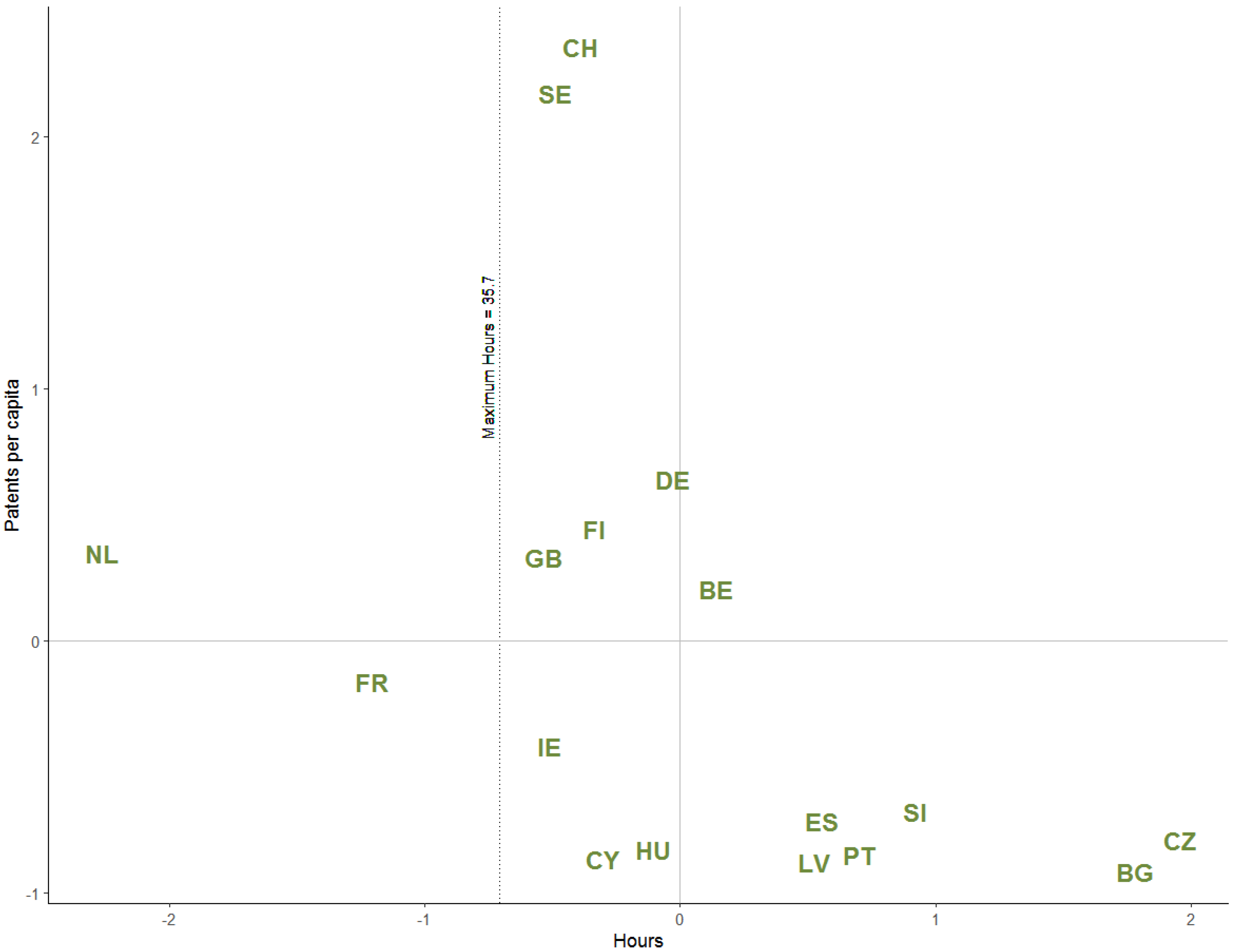
Figure 3 is a plot of country-level per capita patents and work hours (on a standardised scale). The figure shows that Switzerland and Sweden are relatively close to the optimum level of work hours. However, there are other countries, such as Cyprus (CY), with lower innovativeness that are also around the same level. This is not unexpected, as it is clear that work hours alone do not explain differences in innovativeness, an issue that we examine in further detail in Section 5 and Section 6. As shown earlier in Figure 2, Bulgaria and Czechia are countries with high working hours but low innovativeness. Figure 4 displays the same relationship at the regional level. For the sake of readability, we label only those regions that are more than 1.2 standard deviations away from the average hours and those that are more than three standard deviations higher than average per capita patents. The top part of the scatterplot is dotted with highly innovative Swiss regions that are mostly close either to the average hours or to the estimated ideal hours. The Dutch region of Noord-Brabant stands out as a highly innovative region with low working hours (the region of Noord-Brabant has been an important innovation hot spot in the Netherlands [35]). Figure 4 also shows that there is a considerable number of regions with either too long or too short working hours along with low innovativeness.
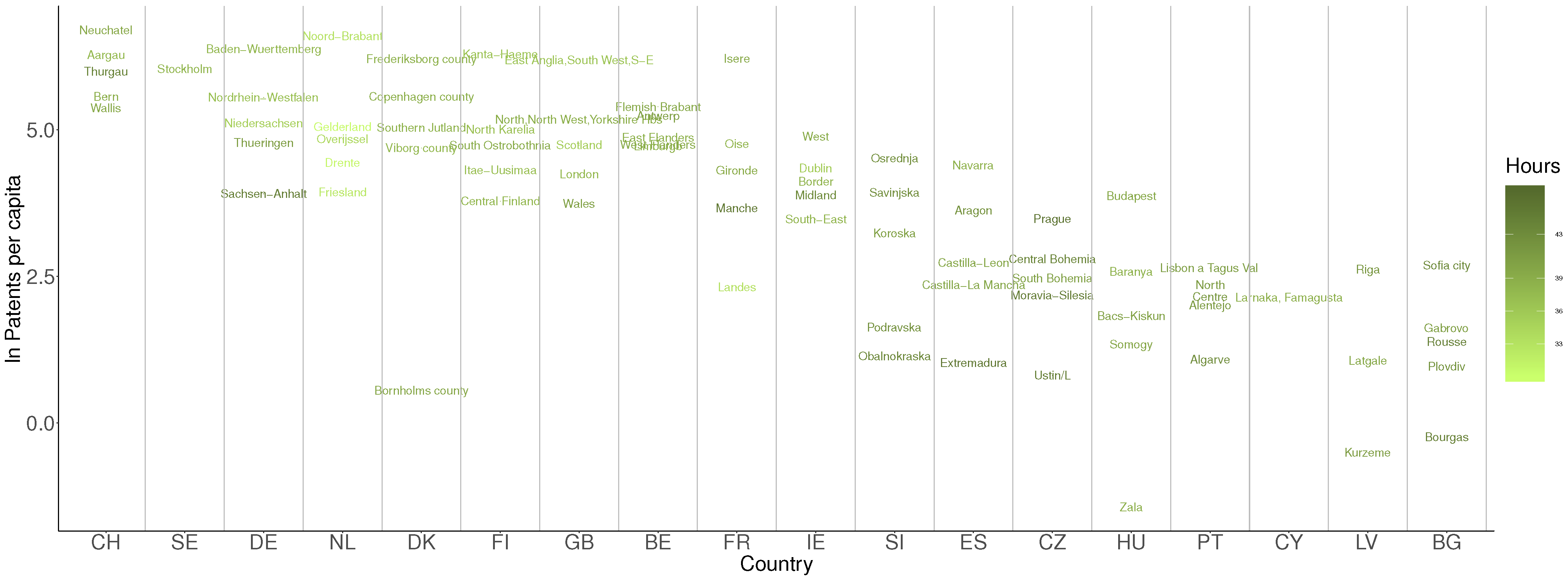
Finally, the levels of innovativeness of regions—ordered by country from high to low—is shown in Figure 5 where darker region labels indicate longer working hours. For each country, only the regions that are in the first, second, and third quartiles and those with the minimum and maximum per capita patent values are shown, provided that they exist in our dataset. As shown earlier in Figure 3, the Netherlands has regions where work hours are low but innovativeness is high. The darker region labels (those with a very high work time effort) are mainly positioned on the right side of the graph where per capita patent values are lower.
In general, the figures presented here hint at a non-linear relationship between work time and innovativeness. This being said, there are clearly other attributes related to the use of work time, in addition to simply the duration of work, e.g., flexibility, freedom to organise one’s workload, and ability to take time off among many other work and location-related factors. Consequently, it is likely that there is a wealth of moderator variables that may impact on creativeness. However, the number of these explanatory variables is simply too large to be meaningfully treated in a standard econometric model; therefore, we will use a simple econometric model as a stepping stone for a more advanced machine learning approach. We aim to revisit and examine the roles of such a larger set of variables through machine learning models in Section 6 by considering the econometric output from Section 5 as a reference point.

5. Spatial Econometric Estimation Results

In this section, we present the results of the econometric model that corresponds to the conceptual model discussed in Section 3. Given the complexity and multidimensionality of the underlying causality patterns, we apply this model later in a complementary machine learning approach, after the estimation of our first-stage regression procedure. As a meaningful point of reference for the statistical performance of the machine learning models, we first estimate a linear regression model augmented with a quadratic term and spatial effects. The quadratic term reflects the inverse U-shaped function discussed in Section 3. Furthermore, this first, non-spatial specification assumes that the observations in one region are independent of observations made in other regions such that if ϵ is the error term of the model, then the assumption is E ( ϵ i ϵ j ) = E ( ϵ i ) E ( ϵ j ) = 0 for two regions i and j [64]. On the other hand, when spatial interdependencies among i and j are considered, for instance, in the case of the outcomes y i and y j , the latter would enter as an explanatory variable for the equation that pertains to the former and vice versa [64]. Considering all locations in the data, the spatial dependencies across all regions can be represented in a spatial autoregressive process by using a spatial weight matrix, as will be detailed in Equation (1) [65]. A spatial model assumes that the inclusion of this spatial autoregressive term ensures that the E ( ε i ε j ) is equal to zero where ε is the error term of the spatial model and that ε N ( 0 , σ 2 ) [64,65].
We begin by implementing a spatial model that is naive in the sense that it ignores endogeneity concerns and accounts only for spatial effects in a simple—and probably misrepresented—form. The former of these shortcomings is basically caused by the fact that all work-related variables from the ISSP survey are already included, and the prospect of successfully finding suitable instrumental variables for them is uncertain, particularly in a cross-sectional setting. The latter drawback is due to the fact that there are some administrative areas among the regions in our sample that are not included in our data. These missing observations would then bias our estimates of indirect spatial effects, and estimating more sophisticated model specifications such as a Spatial Durbin Model in such a context would still be inadequate. Rather than working with econometric models that are semantically not well specified, we will address these concerns in the machine learning (ML) models where they are internalised with a black-box approach. As for simultaneity concerns—i.e., a causal effect of per capita patents on the explanatory variables—we highlight here the fact that there is no clear automatic mechanism that would pressure the managers in a region, on average and from all sectors, to reduce work hours or to increase job flexibility due to a higher number of patents per capita in that region. In essence, this study seeks to acquire new insight into two main elements of information from the econometric estimations for referencing and cross-checking in machine learning procedures: the signs of the coefficient estimates and the optimum number of work hours.
The aforementioned spatial effects are particularly relevant within the context of innovation, growth, and development [66,67,68]. This relevance was theoretically formalised by Ertur and Koch [69], who showed that spatial externalities resulting from the local accumulation of knowledge result in interdependencies among countries. Knowledge spillovers have been observed with greater precision when examined on a disaggregated spatial scale, particularly at the regional level (e.g., [70,71,72,73,74], among others.) Petruzzelli [75] has shown that knowledge spillovers depend on the relative locations of firms and universities in a region. In order to account for spatial dependence in innovativeness, we specify a Spatial Autoregressive Model (SAR):
y = μ ı n + ρ W y + X β + ϵ ϵ N ( 0 , σ 2 )
where y is an N × 1 vector of the natural logarithms of per capita patent applications, and N is the number of observations (N = 253 regions); it is an N × K matrix consisting of K explanatory variables, together with country dummies. The set of variables in X includes explanatory variables that may or may not have a linear effect. However, a “deviation from the optimum” type of specification for these variables (that is, assuming the existence of an optimum level) would not be as straightforward as it is for the case of working hours. The reason for this is that these variables are obtained from individual-level survey responses and subsequently aggregated—or averaged if necessary—to a regional level. Therefore, most of these variables are not individual-level continuous quantitative indicators. Instead, they measure the region-specific share of respondents who responded in a certain manner to a particular question. For instance, as shown in Table 1, the variable Flexible is defined as “the share of respondents who are either completely free to decide the start and end times of their work, or those who have some freedom to decide within certain limits”. The labels, definitions, and the reference categories (when applicable) of all variables are presented in Table 1. Finally, the country-level stock of knowledge, together with other country-level factors such as institutional quality and respect for the rule of law, is represented in the model by the inclusion of country dummies in all subsequent econometric estimations and data-analytical exercises. μ ı n is a constant term, and σ 2 is a constant variance parameter. The work hour variable is introduced in a quadratic form such that its effect is represented in two components: the coefficients of Hours and Hours 2 . In Equation (1), the degree of spatial spillovers of regional innovativeness is evaluated by the parameter estimate ρ . The spatial connectivity is modelled through W, which is an N × N spatial weight matrix. Each element w i j of W is the inverse of the Euclidean distance from the main urban centre of region i to that of region j, and  w i j = 0 if i = j where i = 1 , . . . , N and j = 1 , . . . , N . The aforementioned quadratic definition of the work hours variable aims to capture the potential non-linear effect of this variable and to estimate the ideal length of work time, as outlined in Section 3. The effect of deviating from this optimum length is estimated after replacing the quadratic term with the absolute value of the mean regional deviation from the optimum number of work hours denoted by | z | .
The estimation of a SAR model using ordinary least squares (OLS) would result in biased and inconsistent estimators [76]. To cope with this problem, a maximum likelihood estimation (MLE) that enables asymptotic efficiency is recommended for addressing the bias and inconsistency issues in spatial models [76,77]. That being said, reporting SAR results should be conducted with caution: the direct effect of an explanatory variable appertaining to a certain region on that region’s own innovativeness should be distinguished from the indirect effect of the same variable on the levels of innovativeness in other regions. To be more specific, we follow Elhorst [78] who shows how the direct effects for Equation (1) are calculated as the average of the diagonal elements of ( I ρ W ) 1 β k , which is the partial derivatives matrix with respect to the kth explanatory variable. The indirect effects of k, on the other hand, are given by the mean row (or column) sum of the off-diagonal elements of the same matrix [78]. The direct effects are the same as the SAR coefficients reported in Table 3 up to the second decimal digit, and since there are no significant indirect effects of the explanatory variables, we will simply report the SAR coefficients(the direct, indirect, and total effect breakdown can be provided upon requested). Finally, we also estimate a non-spatial version of Equation (1) (assuming ρ = 0 ) using OLS, and we report the results in the first two columns of Table 3.

Results of the Spatial and Non-Spatial Models

The third and fourth columns of Table 3 present the estimation results of the full model as shown in Equation (1). For both specifications, the results with the quadratic work hour variable are presented first, followed by the estimation results with the deviation from the optimum hours instead. For generating the | z | variable, we use the optimum work hours as estimated by the SAR specification, which is 35.7 h per week.
Firstly, the estimation results in Table 3 highlight a non-linear effect of average regional work hours on innovativeness; work hours affect regional innovativeness positively up to a certain level, but this effect is reversed if work time is too long. The SAR and the non-spatial results are very similar, with the estimate of the optimum work time length being 35.7 h according to the former. The non-linear impact can also be observed when the effect of work hours is expressed as a deviation from this optimum length: Regional innovativeness is reduced as average work hours exceed or fall behind the ideal level (the coefficients estimates on | z | ). The estimated coefficient suggests that a regional average deviation of one hour reduces the per capita patent applications by 5 % .
In contrast to what is found by Beugelsdijk [79], several other variables related to work time such as Flexible, Free, and TimeOff do not appear to yield significant coefficient estimates (however, see [27] for a different perspective). We note here, however, that the machine learning approaches in Section 6 may provide more information regarding the importance of these variables. Nevertheless, the estimation results provide clearer evidence regarding the following: the positive role of the prevalence of the private sector [80]; the share of highly educated individuals [29,81]; the level of urbanization [82,83]; and the weight of the scientific professions in the labor market [84] of a region. Spatial dependence in innovativeness—which should not be over-interpreted, as discussed earlier in this section—is significant and positive, suggesting that there are positive spillovers of knowledge across regions. The associated likelihood ratio and Wald test p-values highlight the significance of the spatial processes in innovativeness and indicate that the spatial specifications should not be reduced to a non-spatial model.
Considering the spatial econometric results presented in Table 3 as a frame of reference, in the next section we aim to provide a deeper understanding of the complex and multidimensional mechanisms that shape regional innovativeness through the application of a collection of machine learning techniques.

6. Machine Learning Applications

Moving from a conventional model-based econometric approach to an algorithmic modelling framework is a big step, as heuristics—rather than an explanatory conceptualisation—comes into play. In fact, the apparent disconnection between the two approaches in the literature was famously outlined by Breiman [85] as the “two cultures” of modeling as opposed to algorithmic learning. While the different cultures are still apparent in economics, over the years the disconnection has lessened, and machine learning has become more accepted in the analysis of economic data [86]. There is a wealth of machine learning (ML) techniques in the current AI literature. Here, we apply five tree-based supervised machine learning methods on our data. Unlike the econometric estimations presented above, ML models necessitate an initial partitioning of the data into two (further discussed below). In order to preserve comparability between the econometric and machine learning applications, we replicate the earlier econometric estimations using the same (partitioned) data as in the machine learning models and compare their root mean squared errors (RMSEs). To further ensure comparability, we run two versions of each machine learning procedure. Firstly, we omit country and spatial effects from the data sets in order to obtain a clearer understanding of strong predictors. Secondly, we rerun the machine learning models including the country dummies and the longitude and latitude values that were used earlier to create the spatial weight matrix W.

6.1. The Base Regression Tree Model

The model of a single regression tree, sketched and applied in this section, serves as the central component of the more powerful ensemble methods that we implement in Section 6.2, Section 6.3 and Section 6.4 (the following R packages were used for applying and visualizing the ML models: rpart by Atkinson and Therneau [87]; randomForest by Breiman and Cutler [88]; xgboost by Chen et al. [89]; rpart.plot by Milborrow [90]; and pdp by Greenwell [91]). A complex, non-linear relationship between the explanatory variables and the dependent variable can be explained better by a regression tree approach compared with a linear regression model, particularly if the causal relationship between these factors is not well approximated by the latter [92,93]. Classification and Regression Trees (CART) provide predictions by splitting the data into subsets [94]. Since the dependent variable is continuous, our models are based on regression trees instead of classification trees. At first, our data are randomly split into two parts: the training data and the test data with shares of 70% and 30%, respectively. Leaving out the test data, a single regression tree uses “recursive binary splitting” in dividing the training data successively in a top-down manner, beginning with an initial split of the data into two regions R 1 ( k , s ) = { X | X k < s } and R 2 ( k , s ) = { X | X k s } , where X k is a selected predictor (out of the earlier-defined K explanatory variables) from the feature space X = ( X 1 , . . . , X K ) , and s is its value used as the first split point [95]. The purpose is then to identify the predictor and splitting value that yields the minimum total of the sum of squared residuals of regions R 1 and R 2 [92,95]:
min k , s i : x i R 1 ( k , s ) ] ( y i y ¯ R 1 ) 2 + i : x i R 2 ( k , s ) ] ( y i y ¯ R 2 ) 2
where y i represents the patent applications per capita for region i; and y ¯ R 1 and y ¯ R 2 are, respectively, the mean values of the same variable for the two data regions (the index term R and the word “region” in this context refers to specific parts or portions of the data split by the ML algorithms and should not be confused with the actual units of observations which are European regions). As the minimisation of the sum of squared residuals (SSR) is performed with respect to the predicted value rather than a slope coefficient, in this framework, the SSR is simply the squared deviations from the mean (see Equation (9).11 in [95]). In other words, the split point decisions aim to minimise the total sum of squares (TSS) (in a tree-based machine learning context, the dependent variable is often called the “outcome”, while the set of explanatory variables, also referred as predictors, make up the “feature space”). Following the initial partitioning of the data, the next step of the recursive binary splitting process is the application of an iterated version of the minimisation in expression (2) to each of the newly identified regions R 1 and R 2 . As a result, the total number of terminal nodes (leaves) R j in this step becomes four. This recursive splitting process stops when a terminal node has too few observations but continues for those regions with a sufficient amount of data. This process yields a large tree that needs to be pruned in order to prevent the overfitting of the data [92,95]. A tree with the highest possible number of splits (i.e., with the highest degree of complexity) would be a full description of the data concerned, resulting in overfitting in a similar manner to a regression where the number of variables is equal to the number of observations, which yields poor out-of-sample predictions [93]. In any case, splitting the data in such a way—which is analogous to using all possible variable interactions in the context of a global parametric equation such as a traditional frequentist regression model—would clearly be a troublesome task to handle the assumption [96,97,98]. A regression tree model, on the other hand, searches automatically for the best interactions and can, therefore, be observed as a “highly interactive function class” due to its local and nonparametric structure [99,100]. The aforementioned pruning process necessary to prevent the overfitting of such a highly interactive specification involves the penalisation (also called “regularisation”) of the size of a tree, measured by its number of terminal nodes | M | . Upon incorporating the complexity parameter ( τ ) into the model, the fully grown tree is pruned by the minimisation of the following:
m = 1 | M | i : x i R m ( y i y ¯ R m ) 2 + τ | M |
where m is the index of the terminal nodes ( m = 1 , . . . , | M | ); and R m is the group of observations that fall into the m’th leaf [92,95]. Therefore, since the error of the tree—summarised by the first term in expression (3)—is inversely related to | M | , the purpose is to find a balance such that the error is as low as possible without fitting an excessively complex tree [92,95].
An optimal value for τ can now be selected following a “K-fold cross-validation” process—as outlined in [92,95]—which randomly splits the observations in the training data into l equal sections ( l = 1 , . . . , L ) (standard notation indexes the “K” folds conveniently by k. We use notation l in order to distinguish this index from the index for the explanatory variables (the K predictors)). Prior to this step, the corresponding unique subtrees that minimise expression (3) are identified for an array of possible values for τ . This step is also applied l times using all the training data except the lth section, and the mean squared prediction errors (MSEs) on the left-out observations are calculated for each level of τ . Due to the fact that in-sample assessment can overstate model accuracy, excluding portions of the data to evaluate model performance is particularly essential [99]. The L number of MSEs are averaged for each level of τ as C V τ = 1 L l = 1 L M S E ( l , τ ) , where C V τ is the cross-validation error function. Finally, the unique subtree of the initially generated unpruned large tree (which uses the full training data) corresponding to the complexity parameter τ that minimises the cross-validation error is used to predict test data [92,95].
The straightforward visual representation of a regression tree allows for a relatively effortless interpretation. However, this method typically has lower predictive accuracy than regression models and may not be robust to changes in the data (i.e., it has a high variance) [92]. Furthermore, in the case of high correlation between model covariates, explanatory variables with a strong relationship to the dependent variable may end up being omitted by the tree model because the splits can be made using other inputs that are highly correlated to those strong predictors [101].
For a preliminary look at the prominence of the variables and the structure of their relationship to per capita patents, we first produce a single regression tree. In addition to the complexity parameter, tuning is required for the minimum number of observations in a terminal node and the maximum depth of the tree (i.e., the maximum number of nodes between the leaves and the root). We conduct a grid search for jointly determining the optimal values for these parameters. The minimum 10-fold cross-validation error corresponds to τ = 0.034 , with a minimum number of five observations and a maximum depth of nine. All tree-based models that we apply use the deviation version of the work duration measure ( | z | ), exclude the quadratic expression for Hours , and include all categories for each predictor (i.e., the exclusion of reference categories is not required).

Regression Tree Results

The single regression tree is presented in Figure 6 where an initial split is made based on Flexible. The predicted level of innovativeness is the least in regions where less than 26 % of individuals do not have any work-hours flexibility. Two other work-time related predictors, Free and | z | , also appear as splitting features. In accordance with our econometric results, innovativeness is predicted to be lower in regions where average work time diverges by about 3 h or more from the optimum level. Additionally, the tree predicts higher innovativeness in regions with a higher share of individuals who have some freedom in their daily work organisation. The model results also reinforce the validity of the econometric findings regarding the positive role of private businesses in reinforcing innovativeness. Finally and not surprisingly, this basic single tree approach suggests that low income is associated with lower regional innovation levels. When the regression tree is constructed after adding country dummies and the longitude and latitude variables in order to increase comparability with the econometric results, it yields an RMSE value of 174.16 . When the econometric estimations are replicated using the same training data and when their prediction performances are tested on the test data, we observed RMSEs ranging from about 110 to 115.
In order to alleviate the above-mentioned drawbacks of using just one regression tree, we now proceed by applying certain appropriate ensemble and sequential techniques for the prediction of per capita patent applications, as outlined in Section 6.2, Section 6.3 and Section 6.4. Ensemble methods combine the predictions of many regression trees resulting in greatly improved predictions [92]. The ensemble methods that we apply on our data are bootstrap aggregation, random forest, and gradient boosting machine learning techniques.

6.2. Bootstrap Aggregation

If the regression tree method is applied on different data sets, such as a new training data set resulting from an alternative random partitioning of the same original data, trees with very different structures and predictions may be reached. This is referred to as “the model having high variance” [92]. The bootstrap aggregation method [102], also called “bagging”, averages over multiple versions of the predicted outcome, each based on a different bootstrap sample drawn with replacement. In our case, bootstrap aggregation is performed by drawing B samples ( b = 1 , , B ) of size N, which is the total number of European regions in the training data. Subsequently, the mean predicted per capita patent application value is calculated. By averaging the outcomes of many tree models—each corresponding to a separate sample b of size N—it is possible to construct a tree-based statistical learning model with a low variance [92]. The bagging estimate of patents per capita for region i is given by y ^ i b a g = 1 B b = 1 B y ^ i , b , where y ^ i , b is the predicted per capita patents for region i resulting from the unpruned unique tree produced by the bth bootstrap sample [92,95].
For each region i in our training data set, there are a number of bootstrap samples (around B 3 ) in which that region is not included [92,103]. In other words, every region is an out of bag (OOB) observation in about one-third of the bootstrap samples [92]. A single estimate of patents per capita for every region can be obtained by averaging their predictions resulting from the samples in which i is OOB (called OOB predictions). In line with this, Svetnik [104] used these OOB predictions to estimate the error rate of the full ensemble.
Ensemble tree methods combine the degree of prominence of each variable resulting from each unique tree by summarising their contribution to the accuracy of the prediction in the form that is called a “variable importance” measure. In a bootstrap aggregation model, the degree of importance of a feature X k is calculated as the mean of the tree-specific decreases in the total of the sum of squared residuals resulting from all binary splits over X k . This degree of importance is then scaled into a 1–100 interval where 100 corresponds to the variable with the highest importance [92]. The outcome of a search for the number of trees that yields the minimum estimated test error (OOB-MSE) suggests using 173 bagged regression trees for obtaining y b a g .

Bootstrap Aggregation Results

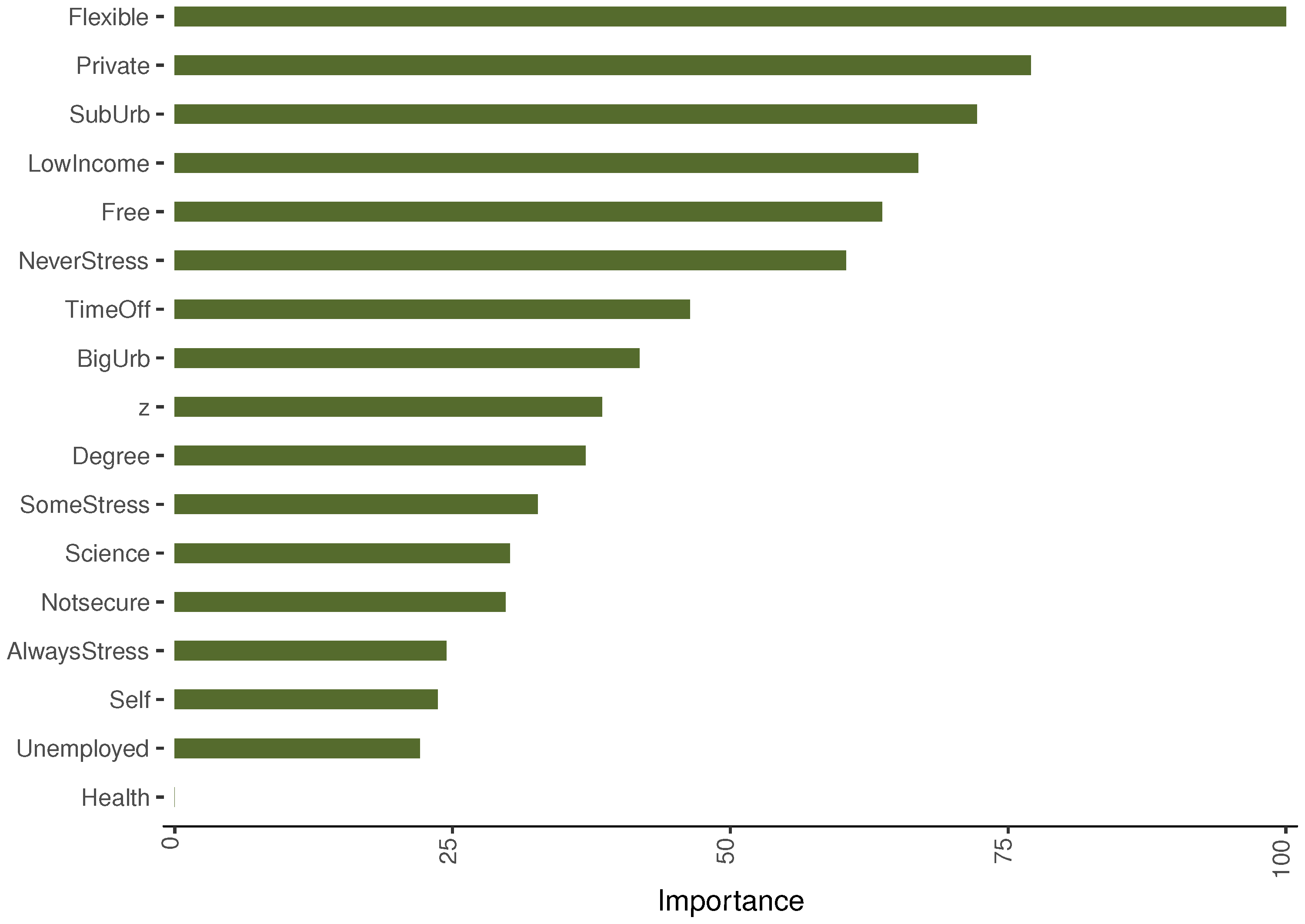
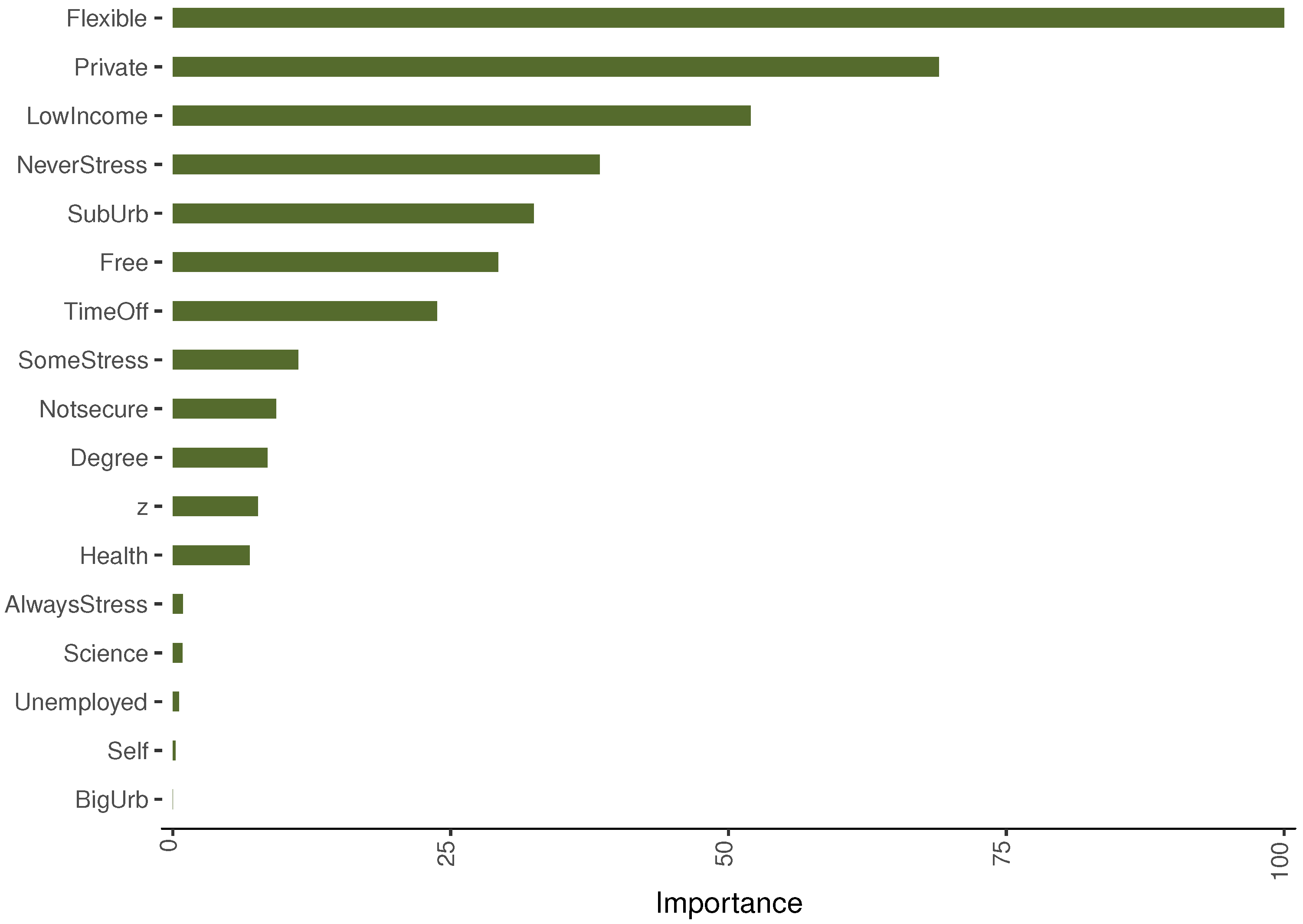
The resulting importance levels of the variables for the bootstrap aggregation model are presented in Figure 7. The flexibility of work hours and the prevalence of the private sector show up as the most important variables. Being in suburban areas and having a low income also appear to be influential in explaining innovativeness. In addition to Flexible, other variables related to work conditions such as Free, TimeOff, and NeverStress strongly contribute to the prediction of per capita patents, along with the other features with lower levels of importance.
When the country and spatial variables are reintroduced, the optimum number of trees becomes 10, and the model yields an RMSE of 137.2214, which is a clear improvement over the single tree model albeit with slightly worse predictions than the econometric results.

6.3. Random Forest

It is reasonable to expect a high degree of correlation among the trees built by the bootstrap aggregation technique, as variables with strong explanatory power will almost always appear as splitters in the top nodes of every tree [92,95]. If the trees are positively correlated, the variance of the average predicted per capita patent values will be ϱ ς 2 + 1 ϱ B ς 2 (instead of only ς 2 B , where ς 2 is the variance for an outcome estimate that is i.i.d.), which can be reduced either by increasing the number of bootstrap sample trees (a higher B) or by reducing correlation coefficient ϱ . The random forest approach, developed by Breiman [103], augments bootstrap aggregation by aiming for the latter before averaging the predictions from each tree for each observation [95,103].
As in the bootstrap aggregation approach, a random forest procedure makes use of a large ensemble of unpruned trees, each based on a bootstrap sample b drawn from the training set. On top of the randomisation introduced by bagging, a random forest procedure introduces further stochasticity by considering only a randomly chosen subset from the feature space at each node of the recursive binary splitting process. The rule of thumb is to calculate—in each binary split step—the best predictor-splitting value combination using only a random sample of q explanatory variables out of the full set of K features, where q = K 3 with a minimum node size of five [95,103].
As in bagging, a random forest procedure evaluates variable importance. Each observation not selected by sample b (i.e., each OOB observation of b) is fitted into the tree corresponding to this sample, and the accuracy of the prediction and the average decrease in MSE is noted. Subsequently, one at a time, the values of each predictor are randomised—keeping the values of the remaining features untouched—and then the decrease in precision as a result of this randomisation is calculated. The loss in accuracy corresponding to a predictor X k is averaged over all trees B, yielding the importance value of its random forest-based variable [103]. Our random forest model, composed of 500 trees with K = 18 and q = 6 and minimum node size of 5, provides further useful information.

Random Forest Results

As presented in the variable importance plot in Figure 8, the random forest results strongly highlight the necessity of flexible work hours. In conjunction with the econometric findings, which provide knowledge regarding whether the predictors are positively or negatively associated with per capita patents, we observe further evidence on the contribution of living in suburban areas, income, the private sector, and the ability to take time off. This random forest model, when augmented with the country and spatial variables, performs with an RMSE of 131.85.
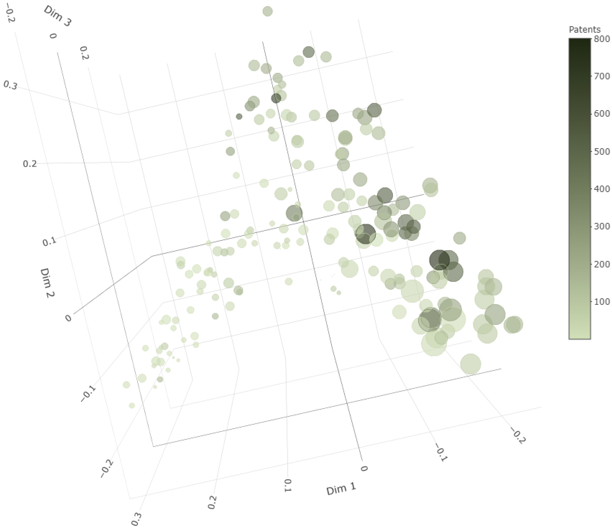
The random forest model can also be used to calculate an inter-observation proximity measure. Returning to the first step in which the OOB observations were run through the tree model from which they were excluded, the random forest model records the pairwise frequency for OOB observations that simultaneously end up in the same terminal node [88,95]. These pairwise frequencies are aggregated over all trees and represented within an N × N matrix after dividing by the total number of trees. The elements of this proximity matrix, when subtracted from one correspond to squared Euclidean distances [88]. Using metric multidimensional scaling, it is possible to express visually the feature-based proximity among the regions in our data set (as opposed to proximity across geographical space) in a lower dimensional space. These proximities are visualised in two-dimensional and three-dimensional plots in Figure 9 and Figure 10, respectively. Regions that are plotted closer to each other have a higher degree of similarity with respect to the predictors, and each arm roughly represents a separate class of regions. Darker coloured region names (and circles in the 3-D version) are those with higher per capita patent applications, and larger circle sizes in Figure 10 represent higher levels of work-time flexibility.

6.4. Stochastic Gradient Boosting Machine

Arguably, among the models that we apply, the “learning” aspect stands out most prominently in a Gradient Boosting Machine (GBM) developed by Friedman [105]. This is due to the GBM’s sequential manner of updating the information learned from each preceding tree. The procedure begins with an initial guess for per capita patents—its sample mean ( y ¯ )—which is the solution to the minimisation of a squared-error loss function. In the sequential framework, the prediction for the European region i made by the preceding tree is denoted as y ^ i , t 1 , where t is the index value for trees ( t = 1 , . . . , T ). The residual r i t which corresponds to observation i from the tree t can be expressed as the negative gradient of the loss function, with respect to the prediction evaluated at each y ^ i , t 1 [106]. Fitting a new regression tree to the residuals r i t yields terminal regions R m t , each generating an average value γ m t (again, a result obtained through the minimisation of a squared-error loss function [95,105]). Therefore, the tree aims to identify those parts of the data where its preceding counterpart made poor predictions [92]. Each preceding prediction is then shifted towards the true value by a step size. The step size for an observation i belonging to region R m t is equal to its predicted residual γ m t weighted by the shrinkage parameter, also called the learning rate, denoted by ν . The learning rate specifies how much each tree learns from previous errors and 0 < ν < 1 . Therefore, if, for instance, a model yields no residuals for a certain group of observations, then there is nothing left for the next model to improve upon the previous predictions. However, if such a claim is false, the subsequent trees can correct this error. Finally, for all i, the gradient boosting algorithm takes the following recursive form:
y ^ i t = y ^ i , t 1 + ν γ m t 1 ( i R m t )
and it is iterated until additional trees no longer improve on preceding predictions [95,105].
For any given observation, the serial mending of the predictions improves the model by rectifying any damage caused by possible missteps taken by the previous tree [107]. Furthermore, the slowdown in the incremental approach introduced by the learning rate provides an opportunity for numerous tree models with various structures to successively tackle model errors [92]. Apart from the learning rate, the other parameters that need to be tuned for a GBM are the number of trees and the interaction depth, which is the number of splits for all trees [92]. A smaller learning rate necessitates the usage of a higher number of trees, and an interaction depth of between 4 and 8 is shown to generally perform well [95,105].
A variant of GBM is a Stochastic Gradient Boosting model (S-GBM). In S-GBM, stochasticity is included into the boosting process by randomly subsampling—without replacement—a portion of the training data at each iteration [106]. Further randomisation can be incorporated into the selection of the split variables at each node in each tree, as in a random forest model. Friedman [106] showed that, in small samples, a learning rate of 0.005 and an optimum number of terminal nodes of seven minimise the estimated error, and a sampling fraction of 0.5 alleviates the consequences of over-fitting that may occur due to large tree sizes. Using the parameter values specified above, we apply the GBM and S-GBM methods—with the sampling fraction being one for the former. We determine the sampling fraction for the feature set at each split as 0.8 for the S-GBM procedure and use a minimum number of five observations in a leaf, with the number of trees being equal to 865 and 324 for GBM and S-GBM, respectively (to complement the suggestions of Friedman [106], the remaining tuning parameters have been determined through a grid search using 10-fold cross validation. Taking a grid search approach for all parameters for GBM and S-GBM is computationally and highly challenging. Thorough grid search-based models may have to run for days using standard personal computers). When spatial and country variables are reintroduced, the RMSE of the GBM is 138.4 , and the S-GBM RMSE is 132.5 . Considering the small number of trees, a manual tweak of the learning rate to 0.1 lowers the latter figure to 125.9 .

GBM and S-GBM Results

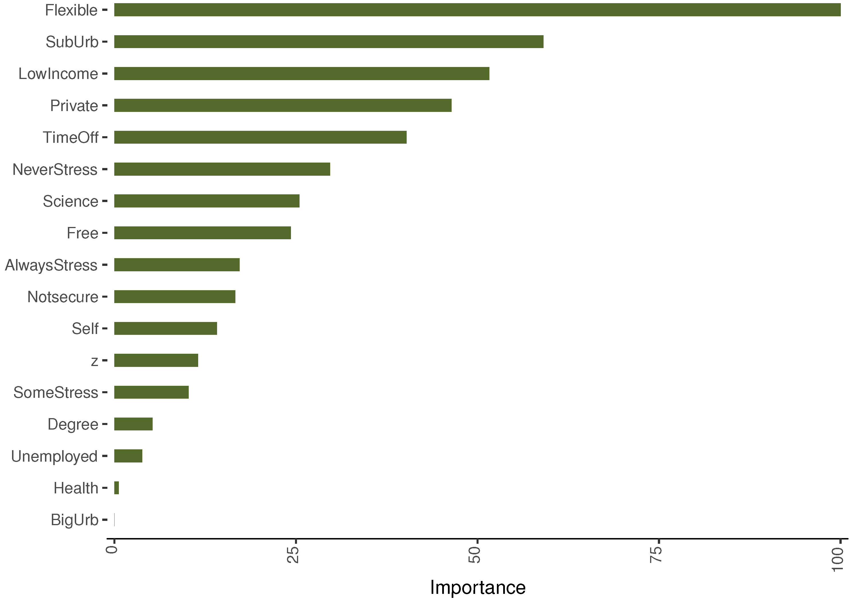
The variable importances based on the GBM and S-GBM are presented in Figure 11 and Figure 12. Both methods rank the variable Flexible as the predictor with the highest importance, as in the bootstrap aggregation and random forest results. The share of private sector employment, suburban residence, income level, and the job-related variables TimeOff and NeverStress appear in the upper half of the list in both models.
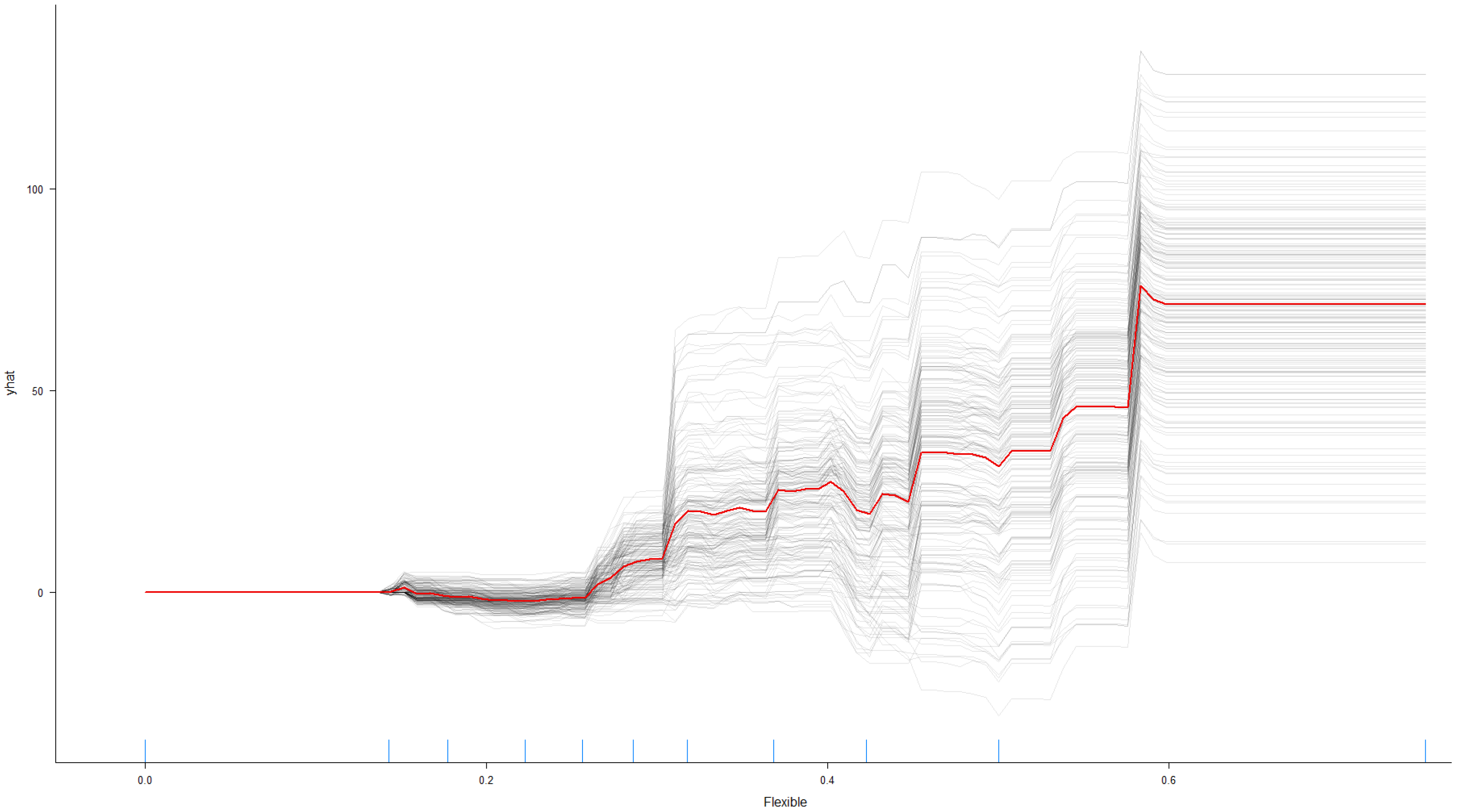
The prominence of the effects of job flexibility and private businesses in our results prompts us to take a closer look at these predictors. The centred individual conditional expectation plot (ICE plot; [108]) in Figure 13 plots the predicted per capita patents versus the variable Flexible, holding all other predictors constant. The partial dependence plot (PDP; [105]) is extended to show the effects of both Flexible and Private, as shown in Figure 14. The average effect of job flexibility is represented by the red line in Figure 13, and the figure suggests that some individual observations demonstrate a differing pattern. The deciles of the variable Flexible are shown by the vertical lines just above the x-axis. While the ICE plot provides further understanding of the relationship, it is important to note that assuming away the correlation between Flexible and the remaining predictors—on which the partial dependence calculation relies—is quite unrealistic, and the figure should not be over-elaborated.
In Figure 14, the values of the predicted per capita patents are distinguished by different colours, with light yellow representing the highest values. The figure suggests that a higher presence of the private sector in a region, coupled with a higher ratio of individuals enjoying job flexibility, may result in greater regional innovativeness.
In summary, the ML techniques employed in this section have uncovered very useful information in addition to the results from the econometric estimations presented earlier. Particularly, the role of job flexibility, the effect of a suburban environment, freedom to organise one’s own work, and the ability to take time off are all identified as important predictors of innovativeness.

7. Conclusions

Innovation is not a top-down process that can be forced. It needs a facilitating and encouraging environment and an open and unconstrained mindset that has to operate in a comfort zone. Against this background, the present study has made an attempt to identify factors that induce individual and group creativeness, such as a flexible work rhythm, freedom to make choices on the work floor, and the like, by specifically examining modern-age work practices just prior to the introduction of advanced smartphones and tablets, which has confounded the concept of flexibility in the subsequent years.
Armbruster [109] had argued that metacognition —the topmost cognitive process that regulates, oversees, and orchestrates cognition—is highly unconscious and that attempting to control and guide individual creativity in too early stages will have a hampering effect. In the same spirit, our findings clearly suggest that innovativeness requires some individual freedom and a flexible work environment. We have observed in our study that an ideal degree of freedom, complemented by a sense of security and a supporting environment, enhances individual and, therefore regional, innovativeness. As a result, our study has extended and further solidified the theoretical relationship between creativity (in the form of regional innovative output) and personal autonomy by examining different dimensions of individual work-related freedom, i.e., the length of work hours, job flexibility, job autonomy, and ability to take time off. Coupled with other individual level factors arising from one’s work such as the levels of stress and the perception of job security, alongside attributes such as the living environment, personal income, and level of education, we have generated new scientific information that can contribute to the extension of the theoretical framework in relation to knowledge production. On the firm level, we have observed the positive role of private businesses. Our results can potentially be added to the pool of evidence together with other research results and influence the labor market side of technology and innovation policies by having an impact on regulations regarding work hours, flexibility, usage of permanent contracts, and support for private establishments.
Undoubtedly, the question of the effect of a relaxed, although responsible, lifestyle at work is too complex to be answered by only one study. Economic, sociological, psychological, and historical viewpoints may need to come together to arrive at a clearer understanding of the individual-level effects of work and place-based geographical factors on innovativeness. There is a clear need for more motivational and cognitive-oriented studies. The current time is characterized by a surge in the availability of Big Data, often in combination with personal perceptions and behavioural stimuli. Against this background, machine learning can serve as a novel and common interdisciplinary methodology for researchers and policy makers in order to understand the individual drivers of creativity and innovation.
Finally, it is remarkable that Elsbach and Hargadon [110] used an analogy from music in their discussion on individual creativity with respect to work design by quoting the jazz musician, Miles Davis, who recognised that the “qualities of musical pieces are not captured in the arrangement of the notes, but also in the arrangement of the silences between notes”. An interesting lesson might be that creative minds should not be put in a position in which they deteriorate due to obstructing or frustrating work and discouraging locational influences. Individual innovativeness should be revived and released, enabling firms, regions, and economies to reach higher levels of welfare.

Author Contributions

Conceptualization, M.G.C., K.K., P.N. and P.-H.W.; methodology, M.G.C. and P.-H.W.; software, M.G.C. and P.-H.W.; validation, M.G.C., K.K., P.N. and P.-H.W.; formal analysis, M.G.C. and P.-H.W.; investigation M.G.C., K.K., P.N. and P.-H.W.; resources, M.G.C., K.K., P.N. and P.-H.W.; data curation, P.-H.W.; writing—original draft preparation, M.G.C., K.K., P.N. and P.-H.W.; writing—review and editing, M.G.C., K.K., P.N. and P.-H.W.; visualization, M.G.C.; supervision, K.K. and P.N.; project administration, K.K. and P.N.; funding acquisition, K.K. and P.N. All authors have read and agreed to the published version of the manuscript.

Funding

Karima Kourtit and Peter Nijkamp gratefully acknowledge the grant from the Romanian Ministry of Research and Innovation, CNCS-UEFISCDI, project number PN-III-P4-ID-PCCF-2016-0166, within the PNCDI III project ReGrowEU—Advancing ground-breaking research in regional growth and development theories through a resilience approach: towards a convergent, balanced and sustainable European Union (Iasi, Romania).

Institutional Review Board Statement

Not applicable.

Informed Consent Statement

Not applicable.

Data Availability Statement

Publicly available datasets were analyzed in this study. This data can be found here: https://ec.europa.eu/eurostat/web/regions/data/database (accessed on 20 September 2021), and https://www.gesis.org/en/issp/modules/issp-modules-by-topic/work-orientations/2005 (accessed on 12 September 2021).

Conflicts of Interest

The authors declare no conflict of interest.

References

  1. Bilbao-Osorio, B.; Rodríguez-Pose, A. From R&D to innovation and economic growth in the EU. Growth Chang. 2004, 35, 434–455. [Google Scholar]
  2. Xiong, A.; Xia, S.; Ye, Z.P.; Cao, D.; Jing, Y.; Li, H. Can innovation really bring economic growth? The role of social filter in China. Struct. Chang. Econ. Dyn. 2020, 53, 50–61. [Google Scholar] [CrossRef]
  3. Asheim, B.T.; Coenen, L. Knowledge bases and regional innovation systems: Comparing Nordic clusters. Res. Policy 2005, 34, 1173–1190. [Google Scholar] [CrossRef]
  4. Etzkowitz, H.; Klofsten, M. The innovating region: Toward a theory of knowledge-based regional development. R D Manag. 2005, 35, 243–255. [Google Scholar] [CrossRef]
  5. Camps, S.; Marques, P. Exploring how social capital facilitates innovation: The role of innovation enablers. Technol. Forecast. Soc. Chang. 2014, 88, 325–348. [Google Scholar] [CrossRef]
  6. Gao, Y.; Zhao, X.; Xu, X.; Ma, F. A study on the cross level transformation from individual creativity to organizational creativity. Technol. Forecast. Soc. Chang. 2021, 171, 120958. [Google Scholar] [CrossRef]
  7. Koh, A.-T. Linking learning, knowledge creation, and business creativity: A preliminary assessment of the East Asian quest for creativity. Technol. Forecast. Soc. Chang. 2000, 64, 85–100. [Google Scholar] [CrossRef]
  8. Li, G.-C.; Lai, R.; D’Amour, A.; Doolin, D.M.; Sun, Y.; Torvik, V.I.; Amy, Z.Y.; Fleming, L. Disambiguation and co-authorship networks of the US patent inventor database (1975–2010). Res. Policy 2014, 43, 941–955. [Google Scholar] [CrossRef]
  9. Barge-Gil, A.; JesusNieto, M.; Santamaria, L. Hidden innovators: The role of non-R&D activities. Technol. Anal. Strateg. Manag. 2011, 23, 415–432. [Google Scholar]
  10. Chesbrough, H.W. Open Innovation: The New Imperative for Creating and Profiting from Technology; Harvard Business Press: Boston, MA, USA, 2003. [Google Scholar]
  11. Hervás-Oliver, J.L.; Parrilli, M.D.; Rodríguez-Pose, A.; Sempere-Ripoll, F. The drivers of SME innovation in the regions of the EU. Res. Policy 2021, 50, 104316. [Google Scholar] [CrossRef]
  12. Santamaría, L.; Nieto, M.J.; Barge-Gil, A. Beyond formal R&D: Taking advantage of other sources of innovation in low-and medium-technology industries. Res. Policy 2009, 38, 507–517. [Google Scholar]
  13. Kourtit, K.; Nijkamp, P. Creative actors and historical–cultural assets in urban regions. Reg. Stud. 2018, 53, 977–990. [Google Scholar] [CrossRef]
  14. Dainow, E. A Concise History of Computers, Smartphones, and the Internet; CreateSpace Independent Publishing Platform: Scotts Valley, CA, USA, 2017. [Google Scholar]
  15. Thulin, E.; Vilhelmson, B.; Johansson, M. New telework, time pressure, and time use control in everyday life. Sustainability 2019, 11, 3067. [Google Scholar] [CrossRef] [Green Version]
  16. Sarwar, M.; Soomro, T.R. Impact of smartphone’s on society. Eur. J. Sci. Res. 2013, 98, 216–226. [Google Scholar]
  17. Derks, D.; van Duin, D.; Tims, M.; Bakker, A.B. Smartphone use and work-home interference: The moderating role of social norms and employee work engagement. J. Occup. Organ. Psychol. 2014, 88, 155–177. [Google Scholar] [CrossRef] [Green Version]
  18. International Labour Organization. Teleworking arrangements during the COVID-19 crisis and beyond. In Proceedings of the 2nd Employment Working Group Meeting under the 2021 Italian Presidency of the G20, online, 14–16 April 2021. [Google Scholar]
  19. Celbiş, M.G.; Crombrugghe, D. Internet infrastructure and regional convergence: Evidence from Turkey. Pap. Reg. Sci. 2018, 97, 387–409. [Google Scholar] [CrossRef]
  20. Türk, U. A multilevel analysis of the contextual effects in distance education outcomes during COVID-19. East. J. Eur. Stud. 2021, 12, 149–169. [Google Scholar] [CrossRef]
  21. Kratzer, J.; Meissner, D.; Roud, V. Open innovation and company culture: Internal openness makes the difference. Technol. Forecast. Soc. Chang. 2017, 119, 128–138. [Google Scholar] [CrossRef]
  22. Ponsiglione, C.; Quinto, I.; Zollo, G. Regional innovation systems as complex adaptive systems: The case of lagging European regions. Sustainability 2018, 10, 2862. [Google Scholar] [CrossRef] [Green Version]
  23. Türkeli, S.; Wong, P.-H.; Yitbarek, E.A. Multiplex learning: An evidence-based approach to design policy learning networks in Sub-Saharan Africa for the SDGs. In Africa and the Sustainable Development Goals; Springer: Berlin/Heidelberg, Germany, 2020; pp. 279–292. [Google Scholar]
  24. Laursen, K.; Foss, N.J. Human resource management practices and innovation. In The Oxford Handbook of Innovation Management; Dodgson, M., Gann, D., Phillips, N., Eds.; Oxford University Press: Oxford, UK, 2014; pp. 505–529. [Google Scholar]
  25. Arvanitis, S. Modes of labor flexibility at firm level: Are there any implications for performance and innovation? Evidence for the Swiss economy. Ind. Corp. Chang. 2005, 14, 993–1016. [Google Scholar] [CrossRef]
  26. Burtch, G.; Carnahan, S.; Greenwood, B.N. Can you gig it? An empirical examination of the gig economy and entrepreneurial activity. Manag. Sci. 2018, 64, 5497–5520. [Google Scholar] [CrossRef] [Green Version]
  27. Arvanitis, S.; Seliger, F.; Stucki, T. The relative importance of human resource management practices for innovation. Econ. Innov. New Technol. 2016, 25, 769–800. [Google Scholar] [CrossRef]
  28. Birkinshaw, J.; Hamel, G.; Mol, M.J. Management innovation. Acad. Manag. Rev. 2008, 33, 825–845. [Google Scholar] [CrossRef]
  29. Kianto, A.; Sáenz, J.; Aramburu, N. Knowledge-based human resource management practices, intellectual capital and innovation. J. Bus. Res. 2017, 81, 11–20. [Google Scholar] [CrossRef]
  30. Suominen, A.; Toivanen, H.; Seppänen, M. Firms’ knowledge profiles: Mapping patent data with unsupervised learning. Technol. Forecast. Soc. Chang. 2017, 115, 131–142. [Google Scholar] [CrossRef] [Green Version]
  31. Ballestar, M.T.; Doncel, L.M.; Sainz, J.; Ortigosa-Blanch, A. A novel machine learning approach for evaluation of public policies: An application in relation to the performance of university researchers. Technol. Forecast. Soc. Chang. 2019, 149, 119756. [Google Scholar] [CrossRef]
  32. Kim, T.S.; Sohn, S.Y. Machine-learning-based deep semantic analysis approach for forecasting new technology convergence. Technol. Forecast. Soc. Chang. 2020, 157, 120095. [Google Scholar] [CrossRef]
  33. Schumpeter, J.A. The Theory of Economic Development; Transaction Publishers: London, UK, 1934. [Google Scholar]
  34. Fagerberg, J.; Srholec, M. National innovation systems, capabilities and economic development. Res. Policy 2008, 37, 1417–1435. [Google Scholar] [CrossRef]
  35. Kourtit, K.; Nijkamp, P.; Lowik, S.; Van Vught, F.; Vulto, P. From islands of innovation to creative hotspots. Reg. Sci. Policy Pract. 2011, 3, 145–161. [Google Scholar] [CrossRef]
  36. Lundvall, B.-Å. National Systems of Innovation: Toward a Theory of Innovation and Interactive Learning; Pinter Publishers: London, UK, 1992. [Google Scholar]
  37. Nelson, R.R. National Innovation Systems: A Comparative Analysis; Oxford University Press: New York, NY, USA, 1993. [Google Scholar]
  38. Leydesdorff, L.; Etzkowitz, H. The triple helix as a model for innovation studies. Sci. Public Policy 1998, 25, 195–203. [Google Scholar]
  39. Cooke, P.; Uranga, M.G.; Etxebarria, G. Regional innovation systems: Institutional and organisational dimensions. Res. Policy 1997, 26, 475–491. [Google Scholar] [CrossRef]
  40. Amabile, T.M.; Conti, R.; Coon, H.; Lazenby, J.; Herron, M. Assessing the work environment for creativity. Acad. Manag. J. 1996, 39, 1154–1184. [Google Scholar]
  41. Laursen, K.; Foss, N.J. New human resource management practices, complementarities and the impact on innovation performance. Camb. J. Econ. 2003, 27, 243–263. [Google Scholar] [CrossRef]
  42. Krammer, S.M. Human resource policies and firm innovation: The moderating effects of economic and institutional context. Technovation 2021, 2, 102366. [Google Scholar] [CrossRef]
  43. Seeck, H.; Diehl, M.R. A literature review on HRM and innovation–taking stock and future directions. Int. J. Hum. Resour. Manag. 2017, 28, 913–944. [Google Scholar] [CrossRef]
  44. Strobel, N.; Kratzer, J. Obstacles to innovation for SMEs: Evidence from Germany. Int. J. Innov. Manag. 2017, 21, 1750030. [Google Scholar] [CrossRef]
  45. Michie, J.; Sheehan, M. Labour market deregulation, ‘flexibility’ and innovation. Camb. J. Econ. 2003, 27, 123–143. [Google Scholar] [CrossRef]
  46. Zhou, H.; Dekker, R.; Kleinknecht, A. Flexible labor and innovation performance: Evidence from longitudinal firm-level data. Ind. Corp. Chang. 2011, 20, 941–968. [Google Scholar] [CrossRef]
  47. Hoxha, S.; Kleinknecht, A. When labour market rigidities are useful for innovation: Evidence from German IAB firm-level data. Res. Policy 2020, 49, 104066. [Google Scholar] [CrossRef]
  48. Hoxha, S.; Kleinknecht, A. Do trustful labor–Management relations enhance innovation? Evidence from German WSI data. Rev. Soc. Econ. 2021, 79, 261–285. [Google Scholar] [CrossRef]
  49. Freeman, C.; Soete, L. The Economics of Industrial Innovation, 3rd ed.; MIT Press: Cambridge, MA, USA, 1997. [Google Scholar]
  50. Celbis, M.G.; Turkeli, S. Does Too Much Work Hamper Innovation? Evidence for Diminishing Returns of Work Hours for Patent Grants. J. Glob. Policy Gov. 2015, 17, 97–116. [Google Scholar]
  51. Cui, D.; Wei, X.; Wu, D.; Cui, N.; Nijkamp, P. Leisure time and labor productivity: A new economic view rooted from sociological perspective. Economics 2019, 13, 1–24. [Google Scholar] [CrossRef] [Green Version]
  52. Jones, C.I. R&D-based models of economic growth. J. Political Econ. 1995, 103, 759–784. [Google Scholar]
  53. Amabile, T.M.; Hadley, C.N.; Kramer, S.J. Creativity under the gun. Harv. Bus. Rev. 2002, 80, 52–63. [Google Scholar]
  54. OECD. Enhancing Productivity in UK Core Cities; OECD: Paris, France, 2020. [Google Scholar]
  55. Glaeser, E.L.; Gottlieb, J.D. The wealth of cities: Agglomeration economies and spatial equilibrium in the United States. J. Econ. Lit. 2009, 47, 983–1028. [Google Scholar] [CrossRef] [Green Version]
  56. Özgüzel, C. Agglomeration Effects in a Developing Country: Evidence from Turkey; Mimeo, Paris School of Economics halshs-02878368; Economic Research Forum: Giza, Egypt, 2020. [Google Scholar]
  57. Celbiş, M.G. A machine learning approach to rural entrepreneurship. Pap. Reg. Sci. 2021, 100, 1079–1104. [Google Scholar] [CrossRef]
  58. Dakhli, M.; DeClercq, D. Human capital, social capital, and innovation: A multi-country study. Entrep. Reg. Dev. 2004, 16, 107–128. [Google Scholar] [CrossRef]
  59. Gu, Y.; Hu, L.; Zhang, H.; Hou, C. Innovation ecosystem research: Emerging trends and future research. Sustainability 2021, 13, 11458. [Google Scholar] [CrossRef]
  60. Szirmai, A.; Naudé, W.; Goedhuys, M. Entrepreneurship, Innovation, and Economic Development; Oxford University Press: Oxford, UK, 2011. [Google Scholar]
  61. ISSP 2005-Work Orientations III Variable Report Documentation Release 2013/07/22. GESIS—Leibniz Institute for the Social Sciences. Archive-Study-No. ZA4350 Version 2.0.0. 2005. Available online: https://www.gesis.org/en/issp/modules/issp-modules-by-topic/work-orientations/2005 (accessed on 20 September 2021).
  62. Buesa, M.; Heijs, J.; Baumert, T. The determinants of regional innovation in Europe: A combined factorial and regression knowledge production function approach. Res. Policy 2010, 39, 722–735. [Google Scholar] [CrossRef]
  63. Bergamini, E.; Zachmann, G. Exploring EU’s regional potential in low-carbon technologies. Sustainability 2021, 13, 32. [Google Scholar] [CrossRef]
  64. LeSage, J.; Pace, R.K. Introduction to Spatial Econometrics; Chapman and Hall/CRC: Boca Raton, FL, USA, 2009. [Google Scholar]
  65. Anselin, L. Spatial Econometrics: Methods and Models; Kluwer Academic Publishers: Dordrecht, The Netherlands, 1988. [Google Scholar]
  66. Celbiş, M.G.; Wong, P.-H.; Guznajeva, T. Regional integration and the economic geography of Belarus. Eurasian Geogr. Econ. 2018, 59, 462–495. [Google Scholar] [CrossRef]
  67. Feldman, M.P. The new economics of innovation, spillovers and agglomeration: A review of empirical studies. Econ. Innov. New Technol. 1999, 8, 5–25. [Google Scholar] [CrossRef]
  68. Fingleton, B.; López-Bazo, E. Empirical growth models with spatial effects. Pap. Reg. Sci. 2006, 85, 177–198. [Google Scholar] [CrossRef]
  69. Ertur, C.; Koch, W. Growth, technological interdependence and spatial externalities: Theory and evidence. J. Appl. Econom. 2007, 22, 1033–1062. [Google Scholar] [CrossRef] [Green Version]
  70. Caragliu, A.; Nijkamp, P. The impact of regional absorptive capacity on spatial knowledge spillovers: The Cohen and Levinthal model revisited. Appl. Econ. 2012, 44, 1363–1374. [Google Scholar] [CrossRef]
  71. Caragliu, A.; Nijkamp, P. Space and knowledge spillovers in European regions: The impact of different forms of proximity on spatial knowledge diffusion. J. Econ. Geogr. 2016, 16, 749–774. [Google Scholar] [CrossRef]
  72. DeDominicis, L.; Florax, R.J.; deGroot, H.L. Regional clusters of innovative activity in Europe: Are social capital and geographical proximity key determinants? Appl. Econ. 2013, 45, 2325–2335. [Google Scholar] [CrossRef]
  73. Fischer, M.M. Regions, technological interdependence and growth in Europe. Rom. J. Reg. Sci. 2009, 3, 1–17. [Google Scholar]
  74. Ponds, R.; van Oort, F.; Frenken, K. Innovation, spillovers and university–Industry collaboration: An extended knowledge production function approach. J. Econ. Geogr. 2009, 10, 231–255. [Google Scholar] [CrossRef]
  75. Petruzzelli, A.M. The impact of technological relatedness, prior ties, and geographical distance on university–industry collaborations: A joint-patent analysis. Technovation 2011, 31, 309–319. [Google Scholar] [CrossRef]
  76. Elhorst, J.P. Specification and estimation of spatial panel data models. Int. Reg. Sci. Rev. 2003, 26, 244–268. [Google Scholar] [CrossRef]
  77. Ord, K. Estimation methods for models of spatial interaction. J. Am. Stat. Assoc. 1975, 70, 120–126. [Google Scholar] [CrossRef]
  78. Elhorst, J.P. Applied spatial econometrics: Raising the bar. Spat. Econ. Anal. 2010, 5, 9–28. [Google Scholar] [CrossRef]
  79. Beugelsdijk, S. Strategic human resource practices and product innovation. Organ. Stud. 2008, 29, 821–847. [Google Scholar] [CrossRef]
  80. Bloch, C.; Bugge, M.M. Public sector innovation—From theory to measurement. Struct. Chang. Econ. Dyn. 2013, 27, 133–145. [Google Scholar] [CrossRef] [Green Version]
  81. D’Este, P.; Rentocchini, F.; Vega-Jurado, J. The role of human capital in lowering the barriers to engaging in innovation: Evidence from the Spanish innovation survey. Ind. Innov. 2014, 21, 1–19. [Google Scholar] [CrossRef]
  82. Beaudry, C.; Schiffauerova, A. Who’s right, Marshall or Jacobs? The localization versus urbanization debate. Res. Policy 2009, 38, 318–337. [Google Scholar] [CrossRef] [Green Version]
  83. Shearmur, R.; Doloreux, D. How open innovation processes vary between urban and remote environments: Slow innovators, market-sourced information and frequency of interaction. Entrep. Reg. Dev. 2016, 28, 337–357. [Google Scholar] [CrossRef]
  84. Chung, S. Building a national innovation system through regional innovation systems. Technovation 2002, 22, 485–491. [Google Scholar] [CrossRef]
  85. Breiman, L. Statistical modeling: The two cultures (with comments and a rejoinder by the author). Stat. Sci. 2001, 16, 199–231. [Google Scholar] [CrossRef]
  86. Imbens, G.; Athey, S. Breiman’s two cultures: A perspective from econometrics. Obs. Stud. 2021, 7, 127–133. [Google Scholar] [CrossRef]
  87. Atkinson, E.J.; Therneau, T.M. An Introduction to Recursive Partitioning Using the RPART Routines; Mayo Foundation: Rochester, NY, USA, 2000. [Google Scholar]
  88. Breiman, L.; Cutler, A. Random Forests. Available online: https://www.stat.berkeley.edu/~breiman/RandomForests/cc_home.htm (accessed on 1 February 2020).
  89. Chen, T.; He, T.; Benesty, M.; Khotilovich, V.; Tang, Y. xgboost: Extreme Gradient Boosting; R Package Version 0.4-2; 2015; pp. 1–4. Available online: http://www.milbo.org/rpart-plot/index.html (accessed on 20 September 2021).
  90. Milborrow, S. R Package ‘Rpart. Plot’; 2019; Available online: https://github.com/dmlc/xgboost (accessed on 20 September 2021).
  91. Greenwell, B.M. pdp: An R package for constructing partial dependence plots. R J. 2017, 9, 421–436. [Google Scholar] [CrossRef] [Green Version]
  92. James, G.; Witten, D.; Hastie, T.; Tibshirani, R. An Introduction to Statistical Learning; Springer: New York, NY, USA, 2013. [Google Scholar]
  93. Varian, H.R. Big data: New tricks for econometrics. J. Econ. Perspect. 2014, 28, 3–28. [Google Scholar] [CrossRef] [Green Version]
  94. Breiman, L.; Friedman, J.H.; Olshen, R.A.; Stone, C.J. Classification and Regression Trees; Wadsworth and Brooks: Monterey, CA, USA, 1984. [Google Scholar]
  95. Friedman, J.; Hastie, T.; Tibshirani, R. The Elements of Statistical Learning; Springer Series in Statistics; Springer: New York, NY, USA, 2001. [Google Scholar]
  96. Collignon, O.; Han, J.; An, H.; Oh, S.; Lee, Y. Comparison of the modified unbounded penalty and the LASSO to select predictive genes of response to chemotherapy in breast cancer. PLoS ONE 2018, 13, e0204897. [Google Scholar] [CrossRef]
  97. Jin, S.; Noh, M.; Lee, Y. H-Likelihood Approach to Factor Analysis for Ordinal Data. Struct. Equ. Model. 2018, 25, 530–540. [Google Scholar] [CrossRef]
  98. Jin, S.; Noh, M.; Yang-Wallentin, F.; Lee, Y. Robust nonlinear structural equation modeling with interaction between exogenous and endogenous latent variables. Struct. Equ. Model. 2021, 28, 1–10. [Google Scholar] [CrossRef]
  99. Mullainathan, S.; Spiess, J. Machine learning: An applied econometric approach. J. Econ. Perspect. 2017, 31, 87–106. [Google Scholar] [CrossRef] [Green Version]
  100. Wong, P.H.; Kourtit, K.; Nijkamp, P. The ideal neighbourhoods of successful ageing: A machine learning approach. Health Place 2021, 72, 102704. [Google Scholar] [CrossRef] [PubMed]
  101. Athey, S.; Imbens, G.W. Machine learning methods that economists should know about. Annu. Rev. Econ. 2019, 11, 685–725. [Google Scholar] [CrossRef]
  102. Breiman, L. Bagging predictors. Mach. Learn. 1996, 24, 123–140. [Google Scholar] [CrossRef] [Green Version]
  103. Breiman, L. Random forests. Mach. Learn. 2001, 45, 5–32. [Google Scholar] [CrossRef] [Green Version]
  104. Svetnik, V.; Liaw, A.; Tong, C.; Wang, T. Application of Breiman’s Random Forest to modeling structure-activity relationships of pharmaceutical molecules. In Multiple Classifier Systems; Lecture Notes in Computer Science; Springer: Berlin/ Heidelberg, Germany, 2004; Volume 3077, pp. 334–343. [Google Scholar]
  105. Friedman, J.H. Greedy function approximation: A gradient boosting machine. Ann. Stat. 2001, 5, 1189–1232. [Google Scholar] [CrossRef]
  106. Friedman, J.H. Stochastic gradient boosting. Comput. Stat. Data Anal. 2002, 38, 367–378. [Google Scholar] [CrossRef]
  107. Schonlau, M. Boosted regression (boosting): An introductory tutorial and a stata plugin. Stata J. 2005, 5, 330–354. [Google Scholar] [CrossRef]
  108. Goldstein, A.; Kapelner, A.; Bleich, J.; Pitkin, E. Peeking inside the black box: Visualizing statistical learning with plots of individual conditional expectation. J. Comput. Graph. Stat. 2015, 24, 44–65. [Google Scholar] [CrossRef]
  109. Armbruster, B.B. Metacognition in creativity. In Handbook of Creativity: Perspectives on Individual Differences; Glover, J., Ronning, R., Reynolds, C., Eds.; Springer: Boston, MA, USA, 1989; pp. 177–182. [Google Scholar]
  110. Elsbach, K.D.; Hargadon, A.B. Enhancing creativity through “mindless” work: A framework of workday design. Organ. Sci. 2006, 17, 470–483. [Google Scholar] [CrossRef] [Green Version]
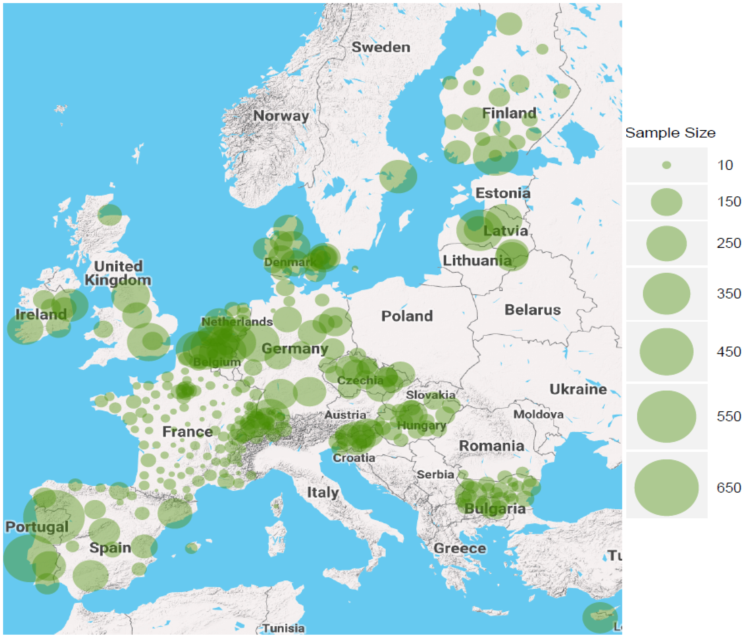
Figure 1. Regions and sample sizes.
Sustainability 13 13426 g001
Figure 2. Patents per capita and hours by country.
Sustainability 13 13426 g002
Figure 3. Patents per capita and hours by country (standardized).
Sustainability 13 13426 g003
Figure 4. Patents per capita and hours by region (standardized).
Sustainability 13 13426 g004
Figure 5. Patents per capita and work hours.
Sustainability 13 13426 g005
Figure 6. Single regression tree.
Sustainability 13 13426 g006
Figure 7. Variable importance: bootstrap aggregation.
Sustainability 13 13426 g007
Figure 8. Variable importance: random forest.
Sustainability 13 13426 g008
Figure 9. Random forest proximity plot: two dimensions.
Sustainability 13 13426 g009
Figure 10. Random forest proximity plot: three dimensions.
Sustainability 13 13426 g010
Figure 11. Variable importance: gradient boosting machine.
Sustainability 13 13426 g011
Figure 12. Variable importance: stochastic gradient boosting machine.
Sustainability 13 13426 g012
Figure 13. Individual conditional expectation plot: job hour flexibility.
Sustainability 13 13426 g013
Figure 14. Individual conditional expectation plot: flexibility and private business.
Sustainability 13 13426 g014
Table 2. Descriptive Statistics.
VariableObsMeanStd. Dev.MinMax
PatCap264127.07160.930.24813.33
Hours30138.884.491055.91
Flexible3010.30.1500.83
Free3010.450.180.021
NotSecure3010.130.0900.5
NeverStress3010.120.0900.75
SomeStress3010.250.1200.8
Science3010.020.0400.23
Private3010.560.1701
Self3010.090.0901
Degree3010.150.1200.75
Unemployed3010.060.0600.31
LowIncome3010.30.1401
BigUrb3010.20.2301
SubUrb3010.10.1700.86
TimeOff3010.380.1601
Health3010.010.0300.25
Table 3. Estimation Results.
Non-SpatialSAR
H o u r s 0.181 *** 0.177 **
(0.050) (0.069)
H o u r s 2 −0.003 *** −0.002 ***
(0.001) (0.001)
| z | −0.051 *** −0.049 ***
(0.015) (0.018)
F l e x i b l e 0.1710.1030.057−0.009
(0.717)(0.717)(0.596)(0.591)
F r e e 0.3870.4500.3390.402
(0.889)(0.880)(0.725)(0.724)
N o t S e c u r e −0.315−0.423−0.318−0.421
(0.650)(0.636)(0.618)(0.614)
N e v e r S t r e s s −0.446−0.508−0.377−0.424
(0.839)(0.796)(0.756)(0.730)
S o m e S t r e s s 0.2720.2240.1440.114
(0.788)(0.738)(0.573)(0.543)
S c i e n c e 3.129 **3.280 **3.063 **3.212 **
(1.307)(1.324)(1.431)(1.422)
P r i v a t e 0.851 **0.875 **0.821 **0.841 **
(0.372)(0.360)(0.392)(0.391)
S e l f −0.572−0.383−0.404−0.238
(0.671)(0.633)(0.638)(0.624)
D e g r e e 1.589 ***1.650 ***1.466 ***1.525 ***
(0.610)(0.613)(0.563)(0.564)
U n e m p l o y e d −2.188−2.738−2.418−2.928
(2.778)(2.824)(1.958)(1.924)
L o w I n c o m e −0.525−0.593−0.528−0.587
(0.556)(0.534)(0.493)(0.484)
B i g U r b 1.005 ***1.001 ***1.035 ***1.031 ***
(0.351)(0.349)(0.292)(0.292)
S u b U r b 0.546 *0.541 *0.4660.463
(0.285)(0.289)(0.316)(0.315)
T i m e O f f −0.071−0.0170.0060.055
(0.625)(0.604)(0.604)(0.595)
H e a l t h −2.636−2.645−2.426−2.413
(2.155)(2.080)(2.070)(2.042)
α 0.7384.082 ***−0.5852.681 **
(1.386)(0.775)(1.818)(1.160)
ρ 0.399 ***0.392 ***
(0.151)(0.151)
Maximum Hours35.9 35.7
Maximum Daily Hours (5-Day)7.2 7.1
RMSE117.4118.3114.2114.8
Observations253253253253
R 2 0.7800.781
Log Likelihood −273.294−272.748
Wald Test p-value 0.0270.009
LR Test p-value 0.0330.037
Notes: Robust standard errors in parentheses: * p < 0.10 , ** p < 0.05 , *** p < 0.01 . To preserve the validity of the reference categories, for each survey variable, the corresponding share of respondents who did not answer is included, but their parameter estimates are not reported.
Publisher’s Note: MDPI stays neutral with regard to jurisdictional claims in published maps and institutional affiliations.