
Quantifying the Response of an Estuarine Nekton Community to Coastal Wetland Habitat Restoration

Abstract
:1. Introduction
2. Materials and Methods
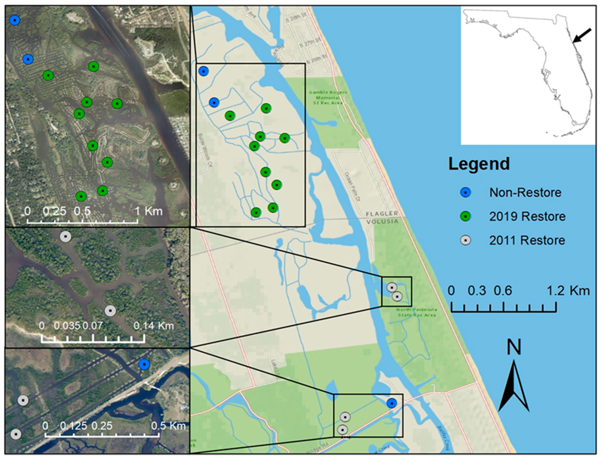
2.1. Study Site
2.2. Biotic Sampling Procedure
2.3. Data Analysis
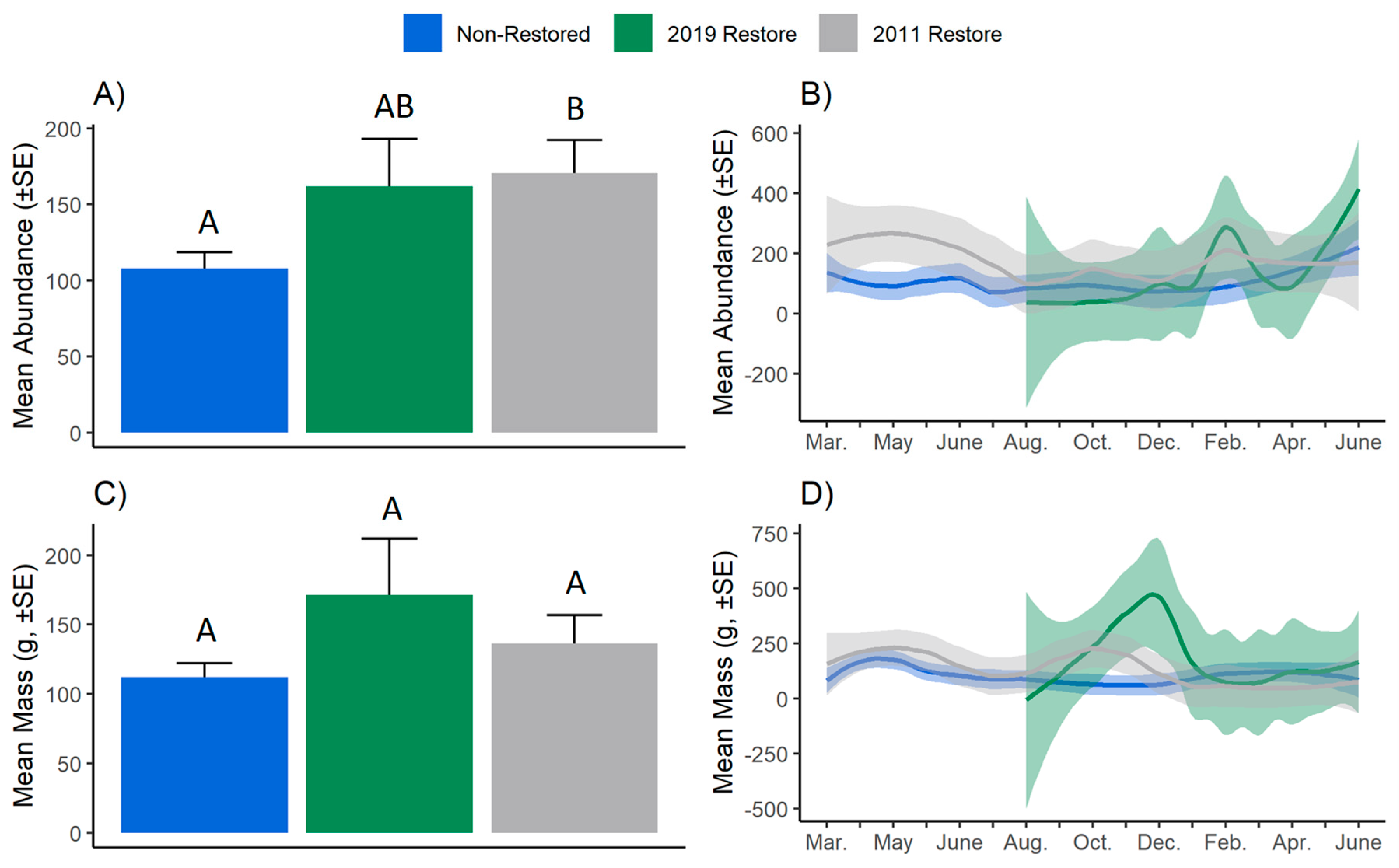
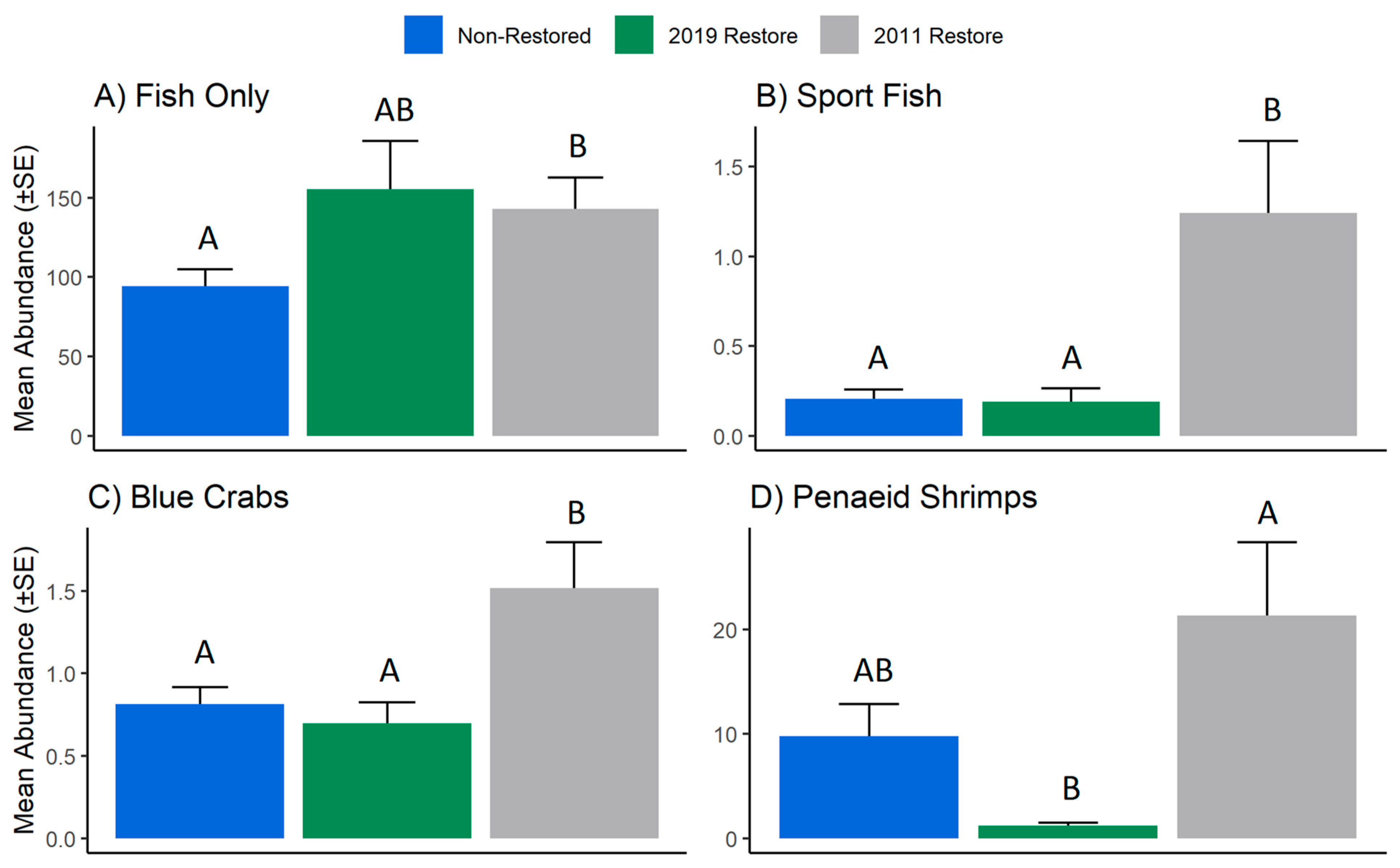
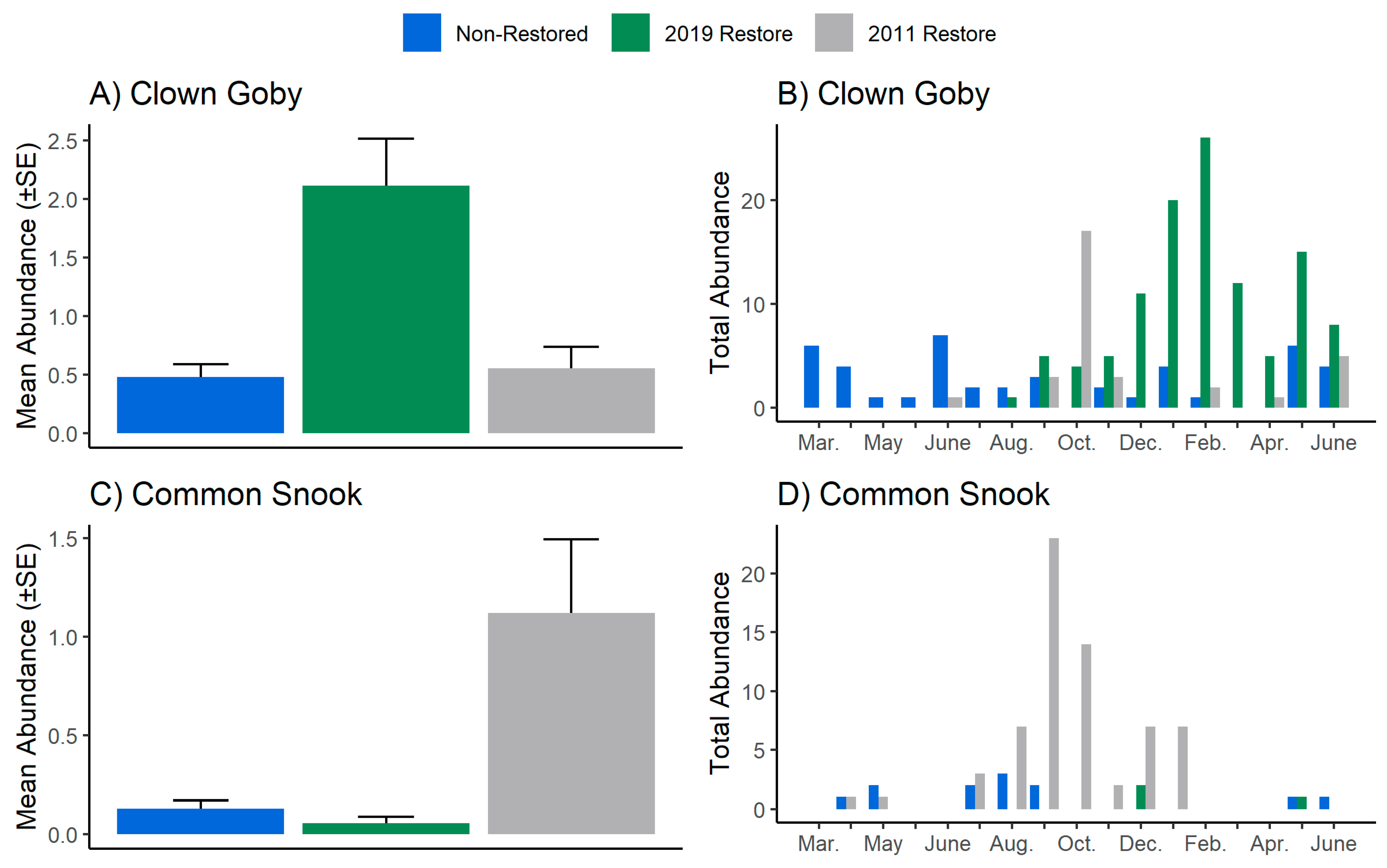
3. Results
4. Discussion
5. Conclusions
Author Contributions
Funding
Institutional Review Board Statement
Data Availability Statement
Acknowledgments
Conflicts of Interest
References
- Travis, J.M.J. Climate change and habitat destruction: A deadly anthropogenic cocktail. Proceedings of the Royal Society of London. Ser. B Biol. Sci. 2003, 270, 467–473. [Google Scholar] [CrossRef] [Green Version]
- Shantz, H.L. The place of grasslands in the Earth’s cover. Ecology 1954, 35, 143–145. [Google Scholar] [CrossRef]
- Repetto, R. Deforestation in the tropics. Sci. Am. 1990, 262, 36–45. [Google Scholar] [CrossRef]
- Beck, M.W.; Heck, K.L.; Able, K.W.; Childers, D.L.; Eggleston, D.B.; Gillanders, B.M.; Halpern, B.; Hays, C.G.; Hoshino, K.; Minello, T.J. The identification, conservation, and management of estuarine and marine nurseries for fish and invertebrates: A better understanding of the habitats that serve as nurseries for marine species and the factors that create site-specific variability in nursery quality will improve conservation and management of these areas. Bioscience 2001, 51, 633–641. [Google Scholar]
- Able, K.W. A re-examination of fish estuarine dependence: Evidence for connectivity between estuarine and ocean habitats. Estuar. Coast. Shelf Sci. 2005, 64, 5–17. [Google Scholar] [CrossRef]
- Li, X.; Bellerby, R.; Craft, C.; Widney, S.E. Coastal wetland loss, consequences, and challenges for restoration. Anthr. Coasts 2018, 1, 1–15. [Google Scholar] [CrossRef] [Green Version]
- Grabowski, J.H.; Peterson, C.H. Restoring oyster reefs to recover ecosystem services. Ecosyst. Eng. Plants Protists 2007, 4, 281–298. [Google Scholar]
- Brown, E.J.; Vasconcelos, R.P.; Wennhage, H.; Bergström, U.; Støttrup, J.G.; van de Wolfshaar, K.; Millisenda, G.; Colloca, F.; Le Pape, O. Conflicts in the coastal zone: Human impacts on commercially important fish species utilizing coastal habitat. ICES J. Mar. Sci. 2018, 75, 1203–1213. [Google Scholar] [CrossRef] [Green Version]
- Dobson, A.; Lodge, D.; Alder, J.; Cumming, G.S.; Keymer, J.; McGlade, J.; Mooney, H.; Rusak, J.A.; Sala, O.; Wolters, V.; et al. Habitat loss, trophic collapse, and the decline of ecosystem services. Ecology 2006, 86, 1915–1924. [Google Scholar] [CrossRef]
- Palmer, M.; Bernhardt, E.; Chornesky, E.; Collins, S.; Dobson, A.; Duke, C.; Gold, B.; Jacobson, R.; Kingsland, S.; Kranz, R.; et al. Ecology for a crowded planet. Science 2004, 304, 1251–1252. [Google Scholar] [CrossRef]
- Worm, B.; Barbier, E.B.; Beaumont, N.; Duffy, J.E.; Folke, C.; Halpern, B.S.; Jackson, J.B.; Lotze, H.K.; Micheli, F.; Palumbi, S.R.; et al. Impacts of biodiversity loss on ocean ecosystem services. Science 2006, 314, 787–790. [Google Scholar] [CrossRef] [Green Version]
- Miller, J.M.; Reed, J.P.; Pietrafesa, L.J. Patterns, mechanisms, and approaches to the study of migrations of estuarine-dependent fish larvae and juveniles. Mech. Migr. Fishes 1984, 14, 209–225. [Google Scholar]
- Lenihan, H.S.; Peterson, C.H. How habitat degradation through fishery disturbance enhances impacts of hypoxia on oyster reefs. Ecol. Appl. 1998, 8, 128–140. [Google Scholar] [CrossRef]
- Sherman, K.; Duda, A.M. An ecosystem approach to global assessment and management of coastal waters. Mar. Ecol. Prog. Ser. 1999, 190, 271–287. [Google Scholar] [CrossRef]
- Lotze, H.K.; Lenihan, H.S.; Bourque, B.J.; Bradbury, R.H.; Cooke, R.G.; Kay, M.C.; Kidwell, S.M.; Kirby, M.X.; Peterson, C.H.; Jackson, J.B. Depletion, degradation, and recovery potential of estuaries and coastal seas. Science 2006, 312, 1806–1809. [Google Scholar] [CrossRef]
- Coen, L.D.; Brumbaugh, R.D.; Bushek, D.; Grizzle, R.; Luckenbach, M.W.; Posey, M.H.; Powers, S.P.; Tolley, S.G. Ecosystem services related to oyster restoration. Mar. Ecol. Prog. Ser. 2007, 341, 303–307. [Google Scholar] [CrossRef]
- Holon, F.; Marre, G.; Parravicini, V.; Mouquet, N.; Bockel, T.; Descamp, P.; Tribot, A.; Boissery, P.; Deter, J. A predictive model based on multiple coastal anthropogenic pressures explains the degradation status of a marine ecosystem: Implication for management and conservation. Biol. Conserv. 2018, 222, 125–135. [Google Scholar] [CrossRef] [Green Version]
- Millennium Ecosystem Assessment (MEA). Ecosystems and Human Well-Being: General Synthesis; World Resources Institute: Washington, DC, USA, 2017. [Google Scholar]
- Lewis, D.M.; Thompson, K.A.; Macdonald, T.C.; Cook, G.S. Understanding Shifts in Estuarine Fish Communities Following Disturbances Using an Ensemble Modeling Framework. Ecol. Indic. 2021, 126, 1–14. [Google Scholar] [CrossRef]
- Thampanya, U.; Vermaat, J.E.; Sinsakul, S.; Panapitukkul, N. Coastal erosion and mangrove progradation of Southern Thailand. Estuar. Coast. Shelf Sci. 2006, 68, 75–85. [Google Scholar] [CrossRef]
- Cook, G.S.; Fletcher, P.J.; Kelble, C.R. Towards marine ecosystem based management in South Florida: Investigating the connections among ecosystem pressures, states, and services in a complex coastal system. Ecol. Indic. 2014, 44, 26–39. [Google Scholar] [CrossRef]
- Rosenberg, A.; Bigford, T.E.; Leathery, S.; Hill, R.L.; Bickers, K. Ecosystem approaches to fishery management through essential fish habitat. Bull. Mar. Sci. 2000, 66, 535–542. [Google Scholar]
- Hsu, S.L.; Wilen, J.E. Ecosystem Management and the 1996 Sustainable Fisheries Act. Ecol. Law Q. 1997, 24, 799. [Google Scholar]
- Robertson, A.I.; Duke, N.C. Mangroves as nursery sites: Comparisons of the abundance and species composition of fish and crustaceans in mangroves and other nearshore habitats in tropical Australia. Mar. Biol. 1987, 96, 193–205. [Google Scholar] [CrossRef]
- Primavera, J.H. Mangroves as nurseries: Shrimp populations in mangrove and non-mangrove habitats. Estuar. Coast. Shelf Sci. 1998, 46, 457–464. [Google Scholar] [CrossRef]
- Lipcius, R.N.; Seitz, R.D.; Seebo, M.S.; Colón-Carrión, D. Density, abundance and survival of the blue crab in seagrass and unstructured salt marsh nurseries of Chesapeake Bay. J. Exp. Mar. Biol. Ecol. 2005, 319, 69–80. [Google Scholar] [CrossRef]
- Sundblad, G.; Bergström, U. Shoreline development and degradation of coastal fish reproduction habitats. Ambio 2014, 43, 1020–1028. [Google Scholar] [CrossRef] [Green Version]
- Lefcheck, J.S.; Hughes, B.B.; Johnson, A.J.; Pfirrmann, B.W.; Rasher, D.B.; Smyth, A.R.; Williams, B.L.; Beck, M.W.; Orth, R.J. Are coastal habitats important nurseries? A meta-analysis. Conserv. Lett. 2019, 12, e12645. [Google Scholar] [CrossRef]
- Orth, R.J.; Heck, K.L.; van Montfrans, J. Faunal communities in seagrass beds: A review of the influence of plant structure and prey characteristics on predator-prey relationships. Estuaries 1984, 7, 339–350. [Google Scholar] [CrossRef]
- Bell, J.D.; Westoby, M. Variation in seagrass height and density over a wide spatial scale: Effects on common fish and decapods. J. Exp. Mar. Biol. Ecol. 1986, 104, 275–295. [Google Scholar] [CrossRef]
- Peterson, G.W.; Turner, R.E. The value of salt marsh edge vs interior as a habitat for fish and decapod crustaceans in a Louisiana tidal marsh. Estuaries 1994, 17, 235–262. [Google Scholar] [CrossRef]
- Minello, T.J.; Able, K.W.; Weinstein, M.P.; Hays, C.G. Salt marshes as nurseries for nekton: Testing hypotheses on density, growth and survival through meta-analysis. Mar. Ecol. Prog. Ser. 2003, 246, 39–59. [Google Scholar] [CrossRef]
- Grabowski, J.H.; Hughes, A.R.; Kimbro, D.L. Habitat complexity influences cascading effects of multiple predators. Ecology 2008, 89, 3413–3422. [Google Scholar] [CrossRef] [Green Version]
- Stunz, G.W.; Minello, T.J.; Rozas, L.P. Relative value of oyster reef as habitat for estuarine nekton in Galveston Bay, Texas. Mar. Ecol. Prog. Ser. 2010, 406, 147–159. [Google Scholar] [CrossRef]
- Gittman, R.K.; Peterson, C.H.; Currin, C.A.; Joel Fodrie, F.; Piehler, M.F.; Bruno, J.F. Living shorelines can enhance the nursery role of threatened estuarine habitats. Ecol. Appl. 2016, 26, 249–263. [Google Scholar] [CrossRef] [PubMed]
- Schulz, K.; Stevens, P.W.; Hill, J.E.; Trotter, A.A.; Ritch, J.L.; Tuckett, Q.M.; Patterson, J.T. Coastal restoration evaluated using dominant habitat characteristics and associated fish communities. PLoS ONE 2020, 15, e0240623. [Google Scholar] [CrossRef]
- Schulz, K.; Stevens, P.W.; Hill, J.E.; Trotter, A.A.; Ritch, J.L.; Williams, K.L.; Patterson, J.T.; Tuckett, Q.M. Coastal wetland restoration improves habitat for juvenile sportfish in Tampa Bay, Florida, USA. Restor. Ecol. 2020, 28, 1283–1295. [Google Scholar] [CrossRef]
- Sullivan, C. The Importance of Mangroves. Department of planning and natural Resources, Division of Fisheries and wildlife. U.S.V.I. Fact Sheet #28. 2005. Available online: http://ufdcimages.uflib.ufl.edu/UF/00/09/34/46/00028/00028Mangroves.pdf (accessed on 1 November 2021).
- Ellison, A.M. Managing mangroves with benthic biodiversity in mind: Moving beyond roving banditry. J. Sea Res. 2008, 59, 2–15. [Google Scholar] [CrossRef]
- Hooke, J.M.; Bray, M.J. Coastal groups, littoral cells, policies and plans in the UK. Area 1995, 27, 358–368. [Google Scholar]
- Lü, Y.; Fu, B.; Feng, X.; Zeng, Y.; Liu, Y.; Chang, R.; Sun, G.; Wu, B. A policy-driven large scale ecological restoration: Quantifying ecosystem services changes in the Loess Plateau of China. PLoS ONE 2012, 7, e31782. [Google Scholar] [CrossRef]
- Zedler, J.B.; Doherty, J.M.; Miller, N.A. Shifting restoration policy to address landscape change, novel ecosystems, and monitoring. Ecol. Soc. 2012, 17. [Google Scholar] [CrossRef] [Green Version]
- Seaman, W. Artificial habitats and the restoration of degraded marine ecosystems and fisheries. Biodivers. Enclosed Seas Artif. Mar. Habitats 2007, 193, 143–155. [Google Scholar]
- Loch, J.M.; Walters, L.J.; Cook, G.S. Recovering trophic structure through habitat restoration: A review. Food Webs 2020, 25, e00162. [Google Scholar] [CrossRef]
- Teas, H.J. Ecology and restoration of mangrove shorelines in Florida. Environ. Conserv. 1977, 4, 51–58. [Google Scholar] [CrossRef]
- Broome, S.W.; Seneca, E.D.; Woodhouse, W.W., Jr. Tidal salt marsh restoration. Aquat. Bot. 1988, 32, 1–22. [Google Scholar] [CrossRef]
- Kondolf, G.M.; Micheli, E.R. Evaluating stream restoration projects. Environ. Manag. 1995, 19, 1–15. [Google Scholar] [CrossRef]
- Kindinger, J.; Flocks, J.; Kulp, M.; Penland, S.; Britsch, L.D.; Brewer, G.; Brooks, G.L.; Dadisman, S.; Dreher, C.; Ferina, N. Sand Resources, Regional Geology, and Coastal Processes for the Restoration of the Barataria Barrier Shoreline (No. 2001-384); US Geological Survey: Reston, VR, USA, 2001. [Google Scholar]
- Ruiz-Jaen, M.C.; Aide, T.M. Restoration success: How is it being measured? Restor. Ecol. 2005, 13, 569–577. [Google Scholar] [CrossRef]
- Cerco, C.F.; Noel, M.R. Can oyster restoration reverse cultural eutrophication in Chesapeake Bay? Estuaries Coasts 2007, 30, 331–343. [Google Scholar] [CrossRef]
- Crooks, S.; Schutten, J.; Sheern, G.D.; Pye, K.; Davy, A.J. Drainage and elevation as factors in the restoration of salt marsh in Britain. Restor. Ecol. 2002, 10, 591–602. [Google Scholar] [CrossRef]
- Brockmeyer, R.E.; Rey, J.R.; Virnstein, R.W.; Gilmore, R.G.; Earnest, L. Rehabilitation of impounded estuarine wetlands by hydrologic reconnection to the Indian River Lagoon, Florida (USA). Wetl. Ecol. Manag. 1996, 4, 93–109. [Google Scholar] [CrossRef]
- Madon, S.P. Fish community responses to ecosystem stressors in coastal estuarine wetlands: A functional basis for wetlands management and restoration. Wetl. Ecol. Manag. 2008, 16, 219–236. [Google Scholar] [CrossRef]
- Bayraktarov, E.; Saunders, M.I.; Abdullah, S.; Mills, M.; Beher, J.; Possingham, H.P.; Mumby, P.J.; Lovelock, C.E. The cost and feasibility of marine coastal restoration. Ecol. Appl. 2016, 26, 1055–1074. [Google Scholar] [CrossRef]
- Cook, G.S.; Heinen, J.T. On the uncertain costs and tenuous benefits of Marine reserves: A case study of the Tortugas Ecological Reserve, South Florida, USA. Nat. Areas J. 2005, 25, 390–396. [Google Scholar]
- Donnelly, M. Effects of Biotic Interactions on Coastal Wetland Communities with Applications for Restoration. Electronic Theses and Dissertations, University of Central Florida, Orlando, FL, USA, 2014. Showcase of Text, Archives, Research and Scholarship. Available online: https://stars.library.ucf.edu/etd/4607 (accessed on 15 November 2020).
- Turner, R.E. Intertidal vegetation and commercial yields of penaeid shrimp. Trans. Am. Fish. Soc. 1977, 106, 411–416. [Google Scholar] [CrossRef]
- Nixon, S.W. Between coastal marshes and coastal waters—A review of twenty years of speculation and research on the role of salt marshes in estuarine productivity and water chemistry. Estuar. Wetl. Process. 1980, 11, 437–525. [Google Scholar]
- Seaman, W. Florida Aquatic Habitat and Fishery Resources; Florida Chapter; American Fisheries Society: New York, NY, USA, 1985. [Google Scholar]
- Zimmerman, R.J.; Minello, T.J.; Rozas, L.P. Salt marsh linkages to productivity of penaeid shrimps and blue crabs in the northern Gulf of Mexico. In Concepts and Controversies in Tidal Marsh Ecology; Springer: Dordrecht, The Netherlands, 2002; pp. 293–314. [Google Scholar]
- Rutledge, K.M.; Alphin, T.; Posey, M. Fish Utilization of Created vs. Natural Oyster Reefs (Crassostrea virginica). Estuaries Coasts 2018, 41, 2426–2432. [Google Scholar] [CrossRef]
- Weinstein, M.P.; Hazen, R.; Litvin, S.Y. Response of Nekton to Tidal Salt Marsh Restoration, a Meta-Analysis of Restoration Trajectories. Wetlands 2019, 39, 575–585. [Google Scholar] [CrossRef]
- Clements, B.W.; Andrew, J. Rogers. Studies of impounding for the control of salt marsh mosquitoes in Florida, 1958-1963. Mosq. News 1964, 24, 265–276. [Google Scholar]
- Stevens, P.W.; Montague, C.L.; Sulak, K.J. Patterns of fish use and piscivore abundance within a reconnected saltmarsh impoundment in the northern Indian River Lagoon, Florida. Wetl. Ecol. Manag. 2006, 14, 147–166. [Google Scholar] [CrossRef]
- Bertness, M.D. The Ecology of Atlantic Shorelines; Sinauer Associates: Sunderland, MA, USA, 1999; p. 417. [Google Scholar]
- Rey, J.R.; Carlson, D.B.; Brockmeyer, R.E. Coastal wetland management in Florida: Environmental concerns and human health. Wetl. Ecol. Manag. 2012, 20, 197–211. [Google Scholar] [CrossRef]
- Balling, S.S.; Resh, V.H. The influence of mosquito control recirculation ditches on plant biomass, production and composition in two San Francisco Bay salt marshes. Estuar. Coast. Shelf Sci. 1983, 16, 151–161. [Google Scholar] [CrossRef]
- Neckles, H.A.; Dionne, M.; Burdick, D.M.; Roman, C.T.; Buchsbaum, R.; Hutchins, E. A monitoring protocol to assess tidal restoration of salt marshes on local and regional scales. Restor. Ecol. 2002, 10, 556–563. [Google Scholar] [CrossRef]
- Okansen, J.; Blanchet, M.F.; Kindt, R.; Legendre, P.; Minchin, P.R.; O’Hara, R.B.; Simpson, G.L.; Solymos, P.; Stevens, M.H.H.; Wagner, H.; et al. Ecology Package “vegan”. Community Ecol. Package 2018, 2, 1–295. [Google Scholar]
- Shannon, C.E. A mathematical theory of communication. Bell Syst. Tech. J. 1948, 27, 379–423. [Google Scholar] [CrossRef] [Green Version]
- Simpson, E.H. Measurement of Diversity. Nature 1949, 163, 688. [Google Scholar] [CrossRef]
- Pielou, E.C. The measurement of diversity in different types of biological collections. J. Theor. Biol. 1966, 13, 131–144. [Google Scholar] [CrossRef]
- Dale, V.H.; Beyeler, S.C. Challenges in the development and use of ecological indicators. Ecol. Indic. 2001, 1, 3–10. [Google Scholar] [CrossRef] [Green Version]
- Gonzalez, E.; Rochefort, L.; Boudreau, S.; Hugron, S.; Poulin, M. Can indicator species predict restoration outcomes early in the monitoring process? A case study with peatlands. Ecol. Indic. 2013, 32, 232–238. [Google Scholar] [CrossRef]
- Cáceres, M.D.; Legendre, P. Associations between species and groups of sites: Indices and statistical inference. Ecology 2009, 90, 3566–3574. [Google Scholar] [CrossRef]
- Zuur, A.F.; Ieno, E.N.; Walker, N.J.; Saveliev, A.A.; Smith, G.M. GLM and GAM for count data. In Mixed Effects Models and Extensions in Ecology with R; Springer: New York, NY, USA, 2009; pp. 209–243. [Google Scholar]
- Fox, J.; Weisberg, S.; Price, B. carData: Companion to Applied Regression Data Sets (3.0-4) [Computer Software]. 2020. Available online: https://CRAN.R-project.org/package=carData (accessed on 1 November 2021).
- Burnham, K.P.; Anderson, D.R. Anderson, D.R. A practical information-theoretic approach. In Model Selection and Multimodel Inference, 2nd ed.; Springer: Berlin/Heidelberg, Germany, 2002. [Google Scholar]
- Turner, R.E.; Lewis, R.R. Hydrologic restoration of coastal wetlands. Wetl. Ecol. Manag. 1996, 4, 65–72. [Google Scholar] [CrossRef]
- Zedler, J.B. Progress in wetland restoration ecology. Trends Ecol. Evol. 2000, 15, 402–407. [Google Scholar] [CrossRef]
- Duever, M.J.; Meeder, J.F.; Meeder, L.C.; McCollum, J.M. The climate of south Florida and its role in shaping the everglades ecosystem. In Everglades: The Ecosystem and Its Restoration; Davis, S.M., Ogden, J.C., Eds.; St. Lucie Press: Delray Beach, FL, USA, 1994; pp. 225–248. [Google Scholar]
- Florida Fish and Wildlife Conservation Commission. 2019. The Economic Impacts of Saltwater Fishing in Florida. Available online: myfwc.com/conservation/value/saltwater-fishing/ (accessed on 22 October 2020).
- Gilmore, R.G.; Cooke, D.W.; Donohoe, C.J. A comparison of the fish populations and habitat in open and closed salt marsh impoundments in east-central Florida. Gulf Mexico Sci. 1982, 5, 2. [Google Scholar] [CrossRef] [Green Version]
- Gilmore, R.G.; Donohoe, C.J.; Cooke, D.W. Observations on the distribution and biology of east-central Florida populations of the common snook, Centropomus undecimalis (Bloch). Florida Sci. 1983, 46, 313–336. [Google Scholar]
- Blewett, D.A.; Stevens, P.W. Temperature variability in a subtropical estuary and implications for common snook Centropomus undecimalis, a cold-sensitive fish. Gulf Mexico Sci. 2014, 32, 4. [Google Scholar] [CrossRef] [Green Version]
- Peters, K.M.; Matheson, R.E., Jr.; Taylor, R.G. Reproduction and early life history of common snook, Centropomus undecimalis (Bloch), in Florida. Bull. Mar. Sci. 1998, 62, 509–529. [Google Scholar]


| Site Type | Indicator Species | A | B | Stat | p-Value | Total # |
|---|---|---|---|---|---|---|
| 2019 Restore | Microgobius gulosus | 0.672 | 0.642 | 0.657 | 0.001 *** | 188 |
| 2011 Restore | Centropomus undecimalis | 0.857 | 0.259 | 0.471 | 0.003 *** | 80 |
| 2019 Restore + 2011 Restore | Menidia spp. | 0.911 | 0.369 | 0.580 | 0.001 ** | 405 |
| 2019 Restore + 2011 Restore | Mugil spp. | 0.927 | 0.324 | 0.548 | 0.001 *** | 861 |
| 2019 Restore + 2011 Restore | Fundulus grandis | 0.947 | 0.108 | 0.325 | 0.015 * | 48 |
| Indicator Species | AIC Best Model | R-Squared |
|---|---|---|
| Microgobius gulosus | site type + salinity + 4 seasons | 0.207 |
| Centropomus undecimalis | site type + salinity + watervolume | 0.1898 |
| Menidia spp. | site type + watervolume | 0.5263 |
| Mugil spp. | site type + salinity + 4 seasons | 0.7338 |
| Fundulus grandis | site type | 0.1675 |
| Category | AIC Best Model | R-Squared |
|---|---|---|
| Abundance | site type + salinity | 0.0768 |
| Richness | null | |
| Shannon Diversity | salinity | 0.0715 |
| Simpson Diversity | salinity | 0.0957 |
| Evenness | salinity + secchi | 0.1379 |
Publisher’s Note: MDPI stays neutral with regard to jurisdictional claims in published maps and institutional affiliations. |
© 2021 by the authors. Licensee MDPI, Basel, Switzerland. This article is an open access article distributed under the terms and conditions of the Creative Commons Attribution (CC BY) license (https://creativecommons.org/licenses/by/4.0/).
Share and Cite
Mahoney, R.D.; Beal, J.L.; Lewis, D.M.; Cook, G.S. Quantifying the Response of an Estuarine Nekton Community to Coastal Wetland Habitat Restoration. Sustainability 2021, 13, 13299. https://doi.org/10.3390/su132313299
Mahoney RD, Beal JL, Lewis DM, Cook GS. Quantifying the Response of an Estuarine Nekton Community to Coastal Wetland Habitat Restoration. Sustainability. 2021; 13(23):13299. https://doi.org/10.3390/su132313299
Chicago/Turabian StyleMahoney, Richard D., Jeffrey L. Beal, Dakota M. Lewis, and Geoffrey S. Cook. 2021. "Quantifying the Response of an Estuarine Nekton Community to Coastal Wetland Habitat Restoration" Sustainability 13, no. 23: 13299. https://doi.org/10.3390/su132313299
APA StyleMahoney, R. D., Beal, J. L., Lewis, D. M., & Cook, G. S. (2021). Quantifying the Response of an Estuarine Nekton Community to Coastal Wetland Habitat Restoration. Sustainability, 13(23), 13299. https://doi.org/10.3390/su132313299