Abstract
Air pollution is among the major causes of death and disease all around the globe. The prime impact of ambient air pollution is on the lungs through the respiratory system. This study aims to estimate the health cost due to air pollution from a Sugar Mill in the Mardan district of Khyber Pakhtunkhwa, Pakistan. To determine the impact of pollution on respiratory illness, primary data were collected from 1141 individuals from 200 households living within a 3 km radius of the mill. The Household Production Method was used to drive the reduced-form Dose–Response Function and the Mitigation Cost Function for assessing the impact of pollution on health and then estimating the monetary cost associated with mitigating such illnesses. The results indicate that about 60% of the respondents living in the surrounding area of the mill suffered from different respiratory illnesses. The study estimates that by reducing the suspended particulate matter (SPM) level by 50%, the expected annual welfare gains to an individual living within a 3 km radius of the mill are US $20.21. The whole community residing within a 3 km radius of the mill will enjoy an estimated welfare gain of PKR. 70.67 million (US $0.511 million). If the pollution standard limits prescribed by the World Health Organization are followed, the expected monetary benefits to all the individuals living within a 3 km radius of the mill are PKR. 114.48 million (US $0.27 million) annually.
1. Introduction
Air pollution is the main reason for the health problems all around the globe, but developing economies are more susceptible to this risk [1]. Air pollution is a complex mixture of gaseous and particulate components, each of which has detrimental effects on cardiovascular and respiratory systems [2]. Individuals in low- and middle-income countries (LMICs) have different exposures, and consequently risk factors, for the development of respiratory diseases as compared with those in higher-income countries [3]. Increased prenatal household air pollution exposure is associated with impaired infant lung function [4]. Worldwide, more than 4 million people die due to diseases from environmental pollution every year [5,6]. Of the total number of deaths, nearly 90% occur in the Asian region, which is the most polluted area in the world, particularly in countries such as China, India, Bangladesh, and Pakistan [5]. According to an estimate, about 4.3 million premature deaths in 2012 were due to air pollution [7]. Of these, 84% were reported to be due to air-pollution-related heart diseases and strokes, 14% were due to pulmonary disease or acute lower respiratory disease, and 6% were due to lung cancer. Later on, new estimates showed that the actual number of premature deaths was 7 million [8]. Particulate matter (PM), a component of air pollution, is a major reason for cancer in humans, and it is closely associated with lung and urinary tract/bladder cancer [9]. A higher level of particulate matter (PM) in the ambient air can reduce the average life expectancy by 50% [10]. A one-unit increase in PM2.5 concentration (µg/m3) is associated with a 9% increase in COVID-19-related mortality [11]. PM2.5 was responsible for 7.3% of all-cause premature deaths in Houston in 2010 [12]. About 500,000 lung cancer deaths and 1.6 million Chronic Obstructive Pulmonary Disease (COPD) deaths were attributed to air pollution, but air pollution may also account for 19% of all cardiovascular deaths and 21% of all stroke deaths [13]. An increase in the average annual Suspended Particulate Matter (SPM) level by <10 µg/m3 (micrograms per meter cubed) increases the mortality rate in adults by 6% [10]. Although air pollution has markedly declined in high-income countries, it was still responsible for some 4.9 million deaths in 2017, largely in low- and middle-income countries where air pollution has increased over the last 25 years [14]. Ambient air pollution reduces the mean life expectancy in Europe by about 2.2 years with an annual attributable per capita mortality rate in Europe of 133/100,000 per year [13].
Industrial pollution is the worst among all pollution types in Pakistan [15]. The poor air quality in Pakistan includes vehicle emissions, solid waste burning, and industrial emissions [16]. Pakistan is currently experiencing economic, demographic, and energy crises; therefore, it has less to spend on environment and water treatment [17]. In addition to this, no serious efforts are put into combating air pollution and the contamination of wastewater from industrial zones. Of the industries in Pakistan, according to Qureshi and Mastoi [18], the sugar industry is the main producer of noise pollution, solid waste, and water pollution. However, less attention had been paid to the air pollution from the sugar industry in Pakistan and its economic impacts.
Pakistan is the fifth-largest sugarcane-producing country in the world and ranks 11th in sugar production. The sugar industry is the second-largest agro-based industry after textiles, employing 10 million people directly and indirectly, the majority of which are from rural areas [19]. On the provincial level, in Khyber Pakhtunkhwa, Premier Sugar Mills Mardan is the biggest sugar producer and has the largest production capacity in Asia. It is situated on the main Nowshera road to Mardan. It became operational in 1951, is run by a board of directors, and has a crushing capacity of 4500 tons/day [20]. However, at the same time, the sugar industry is also responsible for the high concentration of different pollutants in the ambient air emitted during the production process [21]. About 6 kg of fly ash per metric ton of sugarcane processed is produced [22]. Air pollution is the main reason for the different types of respiratory and cardiovascular disease [23]. About 4 million people died due to air pollution [6]. Similarly, pollution is responsible for the reduction in human life expectancy [24], the high rate of mortality and morbidity [25], atherosclerosis [26], and high blood pressure [27]. Some studies indicate that a reduction in such emissions results in benefits to the community in the form of lower health costs (e.g., [28]).
This study focused on the air pollution caused by the emissions from the sugar industry and their contribution to respiratory diseases among the inhabitants of the area surrounding the sugar mill in Mardan district, Khyber Pakhtunkhwa, Pakistan. Furthermore, this study also focused on benefits accruing from a reduction in the pollution to a safe level in the form of reduced health costs to the surrounding residents. The study tested the following hypotheses:
Hypothesis 1 (H1).
The sugar industry is a source of air pollution in the study area.
Hypothesis 2 (H2).
The SMP and other socioeconomic factors of the households are predictors of respiratory illnesses.
Hypothesis 3 (H3).
The SMP and other socioeconomic factors of the households are the predictors of the mitigation cost.
2. Materials and Methods
2.1. Sampling and Study Area
The target area for this research is the area surrounding Premier Sugar Mills Mardan, Khyber Pakhtunkhwa, Pakistan. On the provincial level, it is the largest industrial unit. It became operational in 1951 and has a crushing capacity of 4500 tons/day [20]. For this study, Premier Sugar Mill was selected because this study aimed to conduct a point-source measurement of pollution (a point source is a single emission source at a known location). Premier Sugar Mill is a single unit with no other industry nearby. There is a high probability that the incidence of disease (respiratory illness) in the residents of the surrounding area is due to the pollution from this single unit. So, the effect of reducing air pollution from the sugar mill will have an obvious positive impact on people’s health. The residents in the surrounding area have complained about the black ash or SPM10 (Suspended Particulate Matter having a diameter of <10 μm) in the form of dust that can be observed during daylight. According to the residents, the emission of such dust and ash was controlled several years back with the help of filters in the direction of the environmental department, but after some time it started again. According to the Peshawar report on ambient air quality from the Pakistan Council of Scientific and Industrial Research (PCSIR), Laboratory Khyber Pakhtunkhwa, the mean SPM10 level in the surrounding area of the mill is 266 µg/m3 (micrograms per meter cubed). The standard set by the WHO is an average value of 50 µg/m3 [29] over 24 h, so this level greatly exceeds the standard limit.
For this study, a sample of households was selected using multistage sampling [30]. First of all, from the whole country, the Khyber Pakhtunkhwa Mardan district was purposely selected [31]. In the second stage, the area within a 3-km radius of Premier Sugar Mills Mardan was selected. In the third stage, a sample of households within a 3-km radius (Figure 1) of the mill was taken through simple random sampling. A sample of 200 households was taken using Cochran’s (1977) sample size determination [32]. Keeping in view the “Central Limit Theorem [33]”, the sample size was doubled. Within these 200 households, 1141 individuals’ data were collected.
where n is the number of samples, and is the value for the selected Alpha level of 0.025 in each tail, which is 1.96. The Alpha value shows that there is a 5% chance that the estimated error may cross the acceptance region’s boundaries. (p) × (q) is the estimate of variance (=0.25), with p = 0.5 and q = 0.5. e is the error for the proportion being estimated. As there are resource limitations, the value of “e” is 0.1 [34]. Taking 0.1 as a margin of error is acceptable in social research. For instance, Ullah et al. [35] used a 13% margin of error.
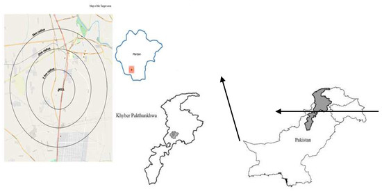
Figure 1.
Study Area Map.
2.2. Data Collection
Household-related data were collected through a well-planned questionnaire through a trained enumerator [36]. The health data were collected from respondents for the last two weeks. The enumerator visited each sample household personally. In the questionnaire, the respondents were requested to provide information about their house structure, socioeconomic characteristics, and health and illnesses.
The pollutant-related data were obtained with the help of the Pakistan Council of Scientific and Industrial Research (PCSIR), Peshawar, Ministry of Science and Technology, Government of Pakistan under Lab Code PLC/FTC/09. The ambient air quality tests were conducted at three points in the target area. Pollution data on Suspended Particulate Matter (PM2.5, PM10) were collected through HAZ DUST, Model EPAM-5000, USA. Sulfur dioxide (SO2) and nitrogen dioxide (NO2), concentrations were measured through Triple Plus, Model 1180, 2003, UK. Carbon monoxide (CO) data were collected through Oldham, Mx21-Plus, made in France. These experiments were conducted by a well-trained technician from PCSIR’s Laboratory. Data were collected during January 2019, which is a wet season. Sugarcane crushing experiences a boom during this month and the mill is operating at its full capacity. Due to the wet season and the mill operating at its full capacity, most of the pollutants, especially SPM, settle down in the nearby surroundings, which can easily be inhaled into the respiratory system. The data were collected at the labor colony (in a 1 km square area), at the college chowk (in a 2 km square area), and in the bank road area (in a 3 km square area), downwind in the direction from south to northeast. Temperature and humidity data were not taken, which is one of the limitations of this study.
2.3. Theoretical Framework
The objectives can be achieved by estimating the Dose–Response Function in order to identify the contribution of different factors to respiratory illnesses among residents of the surrounding area within 3 km of the sugar mill and the Mitigation Cost Function for the calculation of medical and related costs associated with these respiratory diseases. Then, we calculated the benefits or gains from savings in health costs due to the reduction in air pollution emitted from the sugar mill.
This study used the Household Production Function model for the estimation of benefits from the reduction in air pollution emitted from the sugar industry [37,38,39].
An individual’s utility function is given by Equation (2):
where X is a set of consumable market goods, H denotes the health status, and L is the leisure status (Equation (3)). For this function, .
The Health Production Function is as below:
where H is the health status taken as the number of days of illness, A represents aversive activities or preventive measures individuals would take to avoid air pollution, e.g., traveling away from the polluted area or the use of a mask, Q is pollution, and B denotes mitigation activities, which include the doctor’s fee, the medicine cost, and the cost of traveling to the doctor to decrease the impact of the disease.
Substituting the Health Production Function (Equation (3)) into the Utility Function (Equation (2)), Equation (4)) is obtained:
The income (Y) of the individual can be estimated using Equation (5):
where Y is the total income, I is the non-wage income, is the time available after deducting leisure time that is to be spent in the labor market, and w is the wage rate.
The cost function (Equation (6)) can be shown as:
where C represents the cost, X represents units of market goods multiplied by their prices (), A denotes avertive activities, and is the corresponding price per unit of pollution averted. The last term denotes the total cost of mitigation activities. X is treated as a numeraire that is normalized to 1.
Equating the income function (Equation (5)) with the cost function (Equation (6)), we obtain the budget constraint (Equations (7)–(10))
The consumer faces a utility maximization problem subject to the constraint (Equation (11)).
The first-order condition for maximization can be derived with a Lagrange function (Equation (12))
The first-order conditions for maximization are as follows (Equations (13)–(17)).
The first-order condition can be solved for the optimal values of the averting activities (A) mentioned in Equation (18), the medical treatment (B) in Equation (19), the air quality (Q), and the marketable nonenvironmental commodities (X).
The demand for averting activities (A) and medical treatment (B), for example, will take the form
Simultaneous estimation of the Health Production Function (Equations (18) and (19)) yields the Marginal Willingness-to-Pay (MWTP) for the reduction in air quality improvements in Equation (20) [40]:
2.4. Regression Model
In another way, a reduced form of the Dose–Response Function could be estimated, which could then be combined with the estimated Mitigation Cost Function to estimate a lower bound for Equation (20). For these data, only the Health Production Function (the Dose–Response Function) and the Mitigation Expenditure Function (the medical cost function) were estimated.
2.4.1. Dependent Variables
The dependent variables for the Dose–Response Function and the medical and cost functions are as follows:
Dose–Response Function
Equation (21) was estimated for respiratory diseases. If any individual suffered from a respiratory disease in the last two weeks, then otherwise, . Respiratory disease was classified into three types: illnesses or diseases due to air pollution in the upper and lower respiratory systems are denoted upper respiratory illnesses (URI) and lower respiratory illnesses (LRI), respectively, while a person with the symptoms of both an upper and a lower respiratory illness is categorized as having an acute respiratory illness (ARI). The model was estimated three times for each type of disease as a dependent variable. As the outcome of Equation (21) is dichotomous, we used logistic regression analysis. One limitation of logistic regression is that it cannot be interpreted directly. The estimated coefficient’s sign indicates whether the explanatory variables affect the dependent variable (respiratory illness) negatively or positively. For interpretation, odds ratios are reported.
Mitigation Cost Function
The mitigation cost is the amount in Rupees incurred by an individual in the past two weeks for treatment of URI, LRI, and ARI. The model was estimated three times to determine the effect on the mitigation cost for URI, LRI, and ARI. Due to the many zeros for the dependent variable, because the health cost is unknown, OLS regression analysis will result in a biased parameter. To overcome this issue, we applied Tobit regression analysis and censored regression to censor our dependent variable (Equation (22)).
2.4.2. Independent Variables
Smoking Expenditure (smk): Smoking expenditure is the per month expenditure in Rupees spent by individuals. The cost of cigarettes for smokers was calculated by taking the average price per cigarette.
Education level (edu): This variable is categorical. Education level was measured by assigning different values ranging from 1 to 8.
Age (age): Age was represented by a dummy variable. If the individual was between 15 and 55 years, then ‘0’ was assigned. If an individual was less than 15 years or greater than 55 years of age, then ‘1’ was assigned.
Negative Health Stock of last year (nhs): This study tried to associate the health status from the previous year for individuals. This variable took the following dummy form: if the individual suffered from a respiratory illness last year, then nhs = 1; if not, then nhs = 0.
Income (inc): Income was measured in Rupees earned per month by each individual. If the individual was not earning, then it was zero.
Suspended particulate matter (SPM): Suspended particulate matter is the harmful matter emitted by the sugar industry during the production process. The SPM value was measured in micrograms/m3 by skilled technicians from PCSIR laboratories.
Sex (sex): Sex is represented by ‘1’ if an individual was male; otherwise, it is represented by ‘0’.
2.5. Welfare Gains Calculation
In this study, following the procedure suggested by [38,39,41,42], the welfare gains were calculated in the form of a reduction in medical expenditure when the SPM level is decreased from its current to a safe level. So, the annual welfare gain was calculated by reducing the SPM level from the current to a safe level and multiplying it by the SPM coefficient from the mitigation function for that individual whose mitigation cost is > 0.
As and the probability is
then the welfare gain for a two-week period is
and the annual welfare gain is
.
3. Results and Discussion
The results in Table 1 show that in a 1-km radius the PM10 concentration was 433 µg/m3. As the radius was increased, the concentration of PM10 decreased by 109. However, in a 3-km radius, the PM10 concentration was 255 µg/m3. In the 3-km radius, the PM10 concentration was higher than that in the 2-km radius. The reason for this high concentration of PM was the urban area. The population in the 3-km radius was greater than that in the 2-km radius; therefore, there was mill pollution combined with urban pollution. Likewise, the PM2.5 concentration was 318 µg/m3 in a 1-km radius, 160 µg/m3 in a 2-km radius, and 139 µg/m3 in a 3-km radius.

Table 1.
Measurement of pollutants in the ambient air surrounding the mill.
3.1. Descriptive Statistics
Descriptive statistics of both the dependent and independent variables are shown in Table 2. The three dependent variables in the dose–response function, ARI, URI, and LRI, have mean values of 0.14, 0.60, and 0.366, respectively, showing that about 14 percent of respondents suffered from both URI and LRI, which on average cost them PKR.200, while 60 percent and 37 percent suffered only either from an upper respiratory illness or a lower respiratory illness, which cost them PKR.97.18 and PKR.148.04, respectively. The average household consisted of six members and had a monthly income of PKR.27,505. The mean age is about 25 years. About 35% of the individuals fall into the age group of less than 15 years and greater than 55 years, while 65% of the individuals fall into the age group of greater than 15 years and less than 55 years. The results regarding sex show that about 64.3% of respondents were male and 35.7% were female respondents. The literacy rate in the target area was 62.9%. Among these, 7% had less than a primary education. A total of 13% had a primary, a secondary, or a higher secondary education. A total of 4.1% were graduates, while almost 6% were postgraduates. Illiteracy in the target area was reported to be about 37.1%. The data reveal that 5.2% of the respondents were smokers. The average smoking expenditure was PKR.26.98. The negative health stock from the previous year was also incorporated in order to determine its effect on health in the current year. According to the data collected during the survey, pneumonia was reported to be the most expensive in terms of mitigation treatment per individual (PKR.18,357), followed by high blood pressure (PKR.16,212) and heart trouble (PKR.13,750). The incidence of bronchitis was high, and was reported in about 10% of respondents. High blood pressure was reported in about 4.21% of respondents. The average SPM value of both PM10 and PM2.5 was 272.04 µg/m3.
Table 2.
Descriptive statistics of study variables.
3.2. Result of Dose–Response Function
In Table 3, the values of the estimated coefficients of the Logit model are presented. The logistic model resulting from the parameters for each causal variable is presented for each category of disease (ARI, LRI, and URI).
Table 3.
Estimated coefficients of the Dose–Response Function for ARI, LRI, and URI (Logistic Model results).
The estimated results for all three categories show that most of the variables are significant and have the expected sign. Smoking expenditure has a positive impact on increasing the odds of suffering from all three diseases. For ARI and LRI, additional expenditure on smoking will increase the chance of being ill from ARI and LRI by 0.1%, and both were found to be significant at 5%, while for URI, smoking expenditure is significant at 10% with an increase of 0.1% in having URI with an Rs.1 increase in smoking expenditure. For each increase in education grade, the odds of disease rise, but the p-value shows that among these diseases only URI has a significant association with education (at a 5% level of significance). The estimated parameters of age as a dummy variable (if the age less than 15 or greater than 55, then p = 1; otherwise, p = 0) show that the risk of suffering from ARI and URI is 40% (significant at the 10% level) and 76% (significant at the 1% level) higher in the age group of less than 15 and greater than 55. The negative health stock from the previous year showed positive probabilities for ARI and LRI and was significant at the 10% level. The individuals who suffered from any respiratory illness in the previous year were more likely to suffer from ARI and LRI in the current year (40% and 46%, respectively). No statistically significant difference between income and disease (ARI, LRI, and URI) was found to have a positive sign. SPM, which is a crucial variable in the model, showed a positive correlation with all respiratory illnesses (ARI, LRI, and URI). For all three types of respiratory illness, SPM was significant at the 1% level for ARI and URI, and at the 10% level for LRI. According to the odds ratios, a one microgram/m3 emission of SPM in the air increases the odds of suffering from ARI and LRI by 0.1% and URI by 0.2%. Sex, the last variable in the model, shows that URI is significant at the 1% level. The probability of URI was 49% and higher among females compared with males. The results show that the sugar industry caused air pollution in the study area that further led to ARI, LRI, and URI.
3.3. Results of Mitigation Cost Function
Table 4 shows the estimated coefficients of the Mitigation Cost Function for all three dependent variables. Tobit model results show that of the variables, such as smoking expenditure, age, and negative health stock from the previous year, SPM and sex were significant and had the expected sign. An increase in smoking expenditure of Rs.1 increases the mitigation cost by PKR.1.07, 0.52, and 0.18 for ARI, LRI, and URI, respectively. The coefficients for ARI and URI are significant at the 5% level, while the coefficient LRI is significant at the 10% level. These results are in agreement with several earlier studies [41,42,43]. The result for age shows it is significant only for URI (10%). This result matches well with that of Adhikari [41]. Children who are of age 15 or less are more vulnerable to diseases [44]. Similarly, people aged 55 or above are also more vulnerable to disease due to a weak immune system. A similar result was also reported by Adhikari [41].
Table 4.
Estimated coefficients of the Mitigation Cost Function for ARI, LRI, and URI (Tobit Model results).
Risk of illness and cost of illness were both positively correlated to education, although the values were statistically insignificant [41,42]. Education increases the cost of illness on the assumption that education raises awareness regarding disease, so individuals try to obtain the best medical treatment available to them in town. Due to illiteracy, URI was considered a routine illness, so no precautions were usually taken; however, now, due to education, people have become more curious about such illnesses and make regular visits to the doctor. Negative health stock from last year also contributes positively to ARI and LRI. Negative health stock is significant at the 5% and 10% levels for ARI and LRI. The same impact has been reported by many previous studies [41,42]. Income has a positive sign and is statistically insignificant. This implies that rich people, due to the income effect, consume more health services [31,42]. As expected, SPM is the main factor that contributes positively to the cost of illness and is significant at the 1% level for all three categories (ARI, LRI, and URI). Similarly, it also contributes to the health-related costs positively [40].
The final variable, sex, shows that the mitigation cost is high for females compared with males. Sex is significant at the 1% level for URI. The impact of pollution on females was more severe than on males. This result was statistically significant for URI and shows that females are more vulnerable to pollution and that it costs them more. Previous literature also showed the same effect on female health. One of the reasons is that females are more exposed to indoor pollution; therefore, the impact is more obvious.
3.4. Welfare Gains
The estimated annual welfare gains from reducing air pollution are shown in Table 5. The benefits were estimated at three levels: individual, household, and whole community. Similarly, the welfare gains were calculated with different levels of pollution reduction. Five categories were defined (25%, 50%, 75%, 100%, and 81%).
Table 5.
Annual welfare gains in the form of a reduction in the mitigation cost by reducing the average SPM level to various levels.
If the SPM level is reduced by 25%, then an individual residing within a 3-km radius of the factory will save PKR.1397 ($10.12) annually. If a household consists of six members, then benefits at the household level are PKR.8382 ($60.65), which constitutes about 2.6 percent of the annual mean household income. The estimated total population residing within a 3-km radius of the mill is 25,292 [45], so the welfare gain to the whole community would be PKR.35.33 million ($0.256 million) annually.
Reducing the pollution by 50% will lead to a benefit of PKR.2794 ($20.23) per individual, PKR.16,765 ($121.30) per household (almost 5% of a household’s mean annual income), and a total of $0.511 million to the whole community. If pollution is reduced by up to 75% of the current emission level, an individual will be able to save PKR.4191 ($30.32), the family will save PKR.25,147 ($181.94), which is about 7.6 percent of their mean annual income, and the community will be able to save $0.767 million. If the mill stops production, then there will be a 100% reduction in the pollution level and the whole community will obtain a benefit of $1.023 million annually.
If the World Health Organization’s ambient air quality standards are to be properly followed, then the average SPM level has to be reduced to 50 µg/m3 [29]. This implies that the current SPM level has to be reduced by 81%. This reduction in the average SPM level will result in a welfare gain of $0.827 million annually to the whole community. The total welfare gains to an individual in the area surrounding the mill will be PKR.4526. Similarly, the household saving will be PKR.27,158 annually.
3.5. Welfare Gains: A Global Scenario
Different studies have been conducted around the globe, and we compared the results of these studies with our finding ($0.827 million per annum). This number compares well with Bogahawatte and Herath [42], whose results showed a welfare gain of $0.029 million for the Puttalam Cement Factory in Sri Lanka. Some of the estimates suggest that the welfare gain can be much higher depending upon the population of the area. A cross-country comparative analysis shows us that the annual welfare gain from improving the ambient air quality is the highest in Pakistan ($63.44 million), followed by Bangladesh and India ($34.09 million [39] and $7.86 million [46], respectively).
Limitations and Strengths of the Study
This study was conducted in one district (Mardan); in particular, in one of the regions where the sugar industry is located. The results for the other industries may be different. We could not measure the air quality in each household, as a huge budget was needed. The findings will be more robust if measurements can be performed in each household. Furthermore, the findings will be enhanced if the air direction and humidity are also measured. However, this is our first attempt to conduct a study on the sugar industry in Pakistan. This is a baseline study and future studies should work on the limitations of this study and enhance the findings in the future.
4. Conclusions
The emissions from industries are the main reasons for respiratory, cardiovascular, skin, and eye problems. The most disastrous effect of such emissions is cancer, particularly lung cancer. The monetary cost associated with industrial emissions is evident from this study. A reduction in the SPM level contributes to positive social gains. If the ambient air quality standard of 50 micrograms/m3 set by the WHO is followed, an individual would save PKR.4526.29 annually as a decrease in their mitigation cost. Households will obtain an annual benefit of PKR.27,158, while the social welfare gain will be PKR.114.48 million ($0.827 million) per annum. If the SPM level is reduced by 100 percent, then the annual social gain will be PKR.141.34 million ($1.023 million). In addition to these direct benefits from the reduction in the SPM level, there will be some indirect gains in the form of a reduction in the workday’s losses. So, reducing the SPM level has a twofold impact. On the one hand, it reduces the mitigation cost; on the other hand, it increases the social earnings. So, there is a need for the Government to implement a concise policy regarding ambient air quality standards. Current standards do not even comply with the WHO’s standards. Keeping in mind the enormous health cost associated with the emission of SPM into the ambient air estimated in this study, there is a need for policymakers to revise the standards. Alternatively, industries have the option to introduce technologies to abate SPM emissions.
Author Contributions
S.P. and U.A. conceptualized the study. U.A. collected the data and S.P. analyzed it. A.Z. cleaned the data for the analysis and interpreted the results. S.E.S. prepared the first draft of the manuscript. A.U. structured the manuscript and edited it. M.R. supervised the entire research process and provided inputs to all of the authors. All authors have read and agreed to the published version of the manuscript.
Funding
The authors did not receive funding for the authorship and/or publication of this study.
Institutional Review Board Statement
Not applicable.
Informed Consent Statement
Not applicable.
Data Availability Statement
The data and materials used in this study are available upon request to the corresponding author.
Acknowledgments
The authors are grateful to all of the study participants who gave their time for the interviews.
Conflicts of Interest
The authors declare no conflict of interest with respect to the research, authorship, and/or publication of this study.
References
- Manisalidis, I.; Stavropoulou, E.; Stavropoulos, A.; Bezirtzoglou, E. Environmental and health impacts of air pollution: A review. Front. Public Health 2020, 8, 14. [Google Scholar] [CrossRef] [Green Version]
- Hamanaka, R.B.; Mutlu, G.M. Particulate matter air pollution: Effects on the cardiovascular system. Front. Endocrinol. 2018, 9, 680. [Google Scholar] [CrossRef] [PubMed] [Green Version]
- Sui, G.; Liu, G.; Jia, L.; Wang, L.; Yang, G. The association between ambient air pollution exposure and mental health status in Chinese female college students: A cross-sectional study. Environ. Sci. Pollut. Res. 2018, 25, 28517–28524. [Google Scholar] [CrossRef]
- Lee, A.G.; Kaali, S.; Quinn, A.; Delimini, R.; Burkart, K.; Opoku-Mensah, J.; Wylie, B.J.; Yawson, A.K.; Kinney, P.L.; Ae-Ngibise, K.A. Prenatal household air pollution is associated with impaired infant lung function with sex-specific effects. Evidence from graphs, a cluster randomized Cookstove intervention trial. Am. J. Respir. Crit. Care Med. 2019, 199, 738–746. [Google Scholar] [PubMed]
- Khan, S.A.R.; Sharif, A.; Golpîra, H.; Kumar, A. A green ideology in Asian emerging economies: From environmental policy and sustainable development. Sustain. Dev. 2019, 27, 1063–1075. [Google Scholar] [CrossRef]
- Li, X.; Jin, L.; Kan, H. Air pollution: A global problem needs local fixes. Nature 2019, 570, 437–439. [Google Scholar] [CrossRef] [Green Version]
- WHO. Burden of Disease from Household Air Pollution for 2012. 2014. Available online: http://www.who.int/phe/health_topics/outdoorair/databases/FINAL_HAP_AAP_BoD_24March2014.pdf?ua=1 (accessed on 21 December 2020).
- WHO. 7 Million Premature Deaths Annually Linked to Air Pollution. 2014. Available online: http://www.who.int/mediacentre/news/releases/2014/air-pollution/en/ (accessed on 21 December 2020).
- Loomis, D.; Huang, W.; Chen, G. The International Agency for Research on Cancer (IARC) evaluation of the carcinogenicity of outdoor air pollution: Focus on China. Chin. J. Cancer 2014, 33, 189. [Google Scholar] [CrossRef]
- Krewski, D.; Jerrett, M.; Burnett, R.T.; Ma, R.; Hughes, E.; Shi, Y.; Turner, M.C.; Pope, C.A., III; Thurston, G.; Calle, E.E. Extended Follow-Up and Spatial Analysis of the American Cancer Society Study Linking Particulate Air Pollution and Mortality; Health Effects Institute: Boston, MA, USA, 2009.
- Coker, E.S.; Cavalli, L.; Fabrizi, E.; Guastella, G.; Lippo, E.; Parisi, M.L.; Pontarollo, N.; Rizzati, M.; Varacca, A.; Vergalli, S. The effects of air pollution on COVID-19 related mortality in northern Italy. Environ. Resour. Econ. 2020, 76, 611–634. [Google Scholar] [CrossRef] [PubMed]
- Sohrabi, S.; Zietsman, J.; Khreis, H. Burden of Disease Assessment of Ambient Air Pollution and Premature Mortality in Urban Areas: The Role of Socioeconomic Status and Transportation. Int. J. Environ. Res. Public Health 2020, 17, 1166. [Google Scholar] [CrossRef] [Green Version]
- Lelieveld, J.; Klingmüller, K.; Pozzer, A.; Pöschl, U.; Fnais, M.; Daiber, A.; Münzel, T. Cardiovascular disease burden from ambient air pollution in Europe reassessed using novel hazard ratio functions. Eur. Heart J. 2019, 40, 1590–1596. [Google Scholar] [CrossRef] [PubMed] [Green Version]
- Boogaard, H.; Walker, K.; Cohen, A.J. Air pollution: The emergence of a major global health risk factor. Int. Health 2019, 11, 417–421. [Google Scholar] [CrossRef] [PubMed]
- Mehdi, M.A. Industrial Pollution in Pakistan. 2019. Available online: https://nation.com.pk/07-Jan-2019/industrial-pollution-in-pakistan (accessed on 7 October 2021).
- AIMAT. Pakistan General Health Risks: Air Pollution; International Association for Medical Assistance to Travellers: New York, NY, USA, 2020. [Google Scholar]
- Mahmood, Q.; Shaheen, S.; Bilal, M.; Tariq, M.; Zeb, B.S.; Ullah, Z.; Ali, A. Chemical pollutants from an industrial estate in Pakistan: A threat to environmental sustainability. Appl. Water Sci. 2019, 9, 47. [Google Scholar] [CrossRef] [Green Version]
- Qureshi, M.A.; Mastoi, G.M. The physiochemistry of sugar mill effluent pollution of coastlines in Pakistan. Ecol. Eng. 2015, 75, 137–144. [Google Scholar] [CrossRef]
- Rehman, M.S.U. Pakistan Sugar Annual 2016. Available online: https://gain.fas.usda.gov/Recent%20GAIN%20Publications/Sugar%20Annual_Islamabad_Pakistan_4-27-2016.pdf (accessed on 1 December 2016).
- Mardan Sugar Mill. Profile of the Company. 2019. Available online: http://premiersugarmills.com/index.html (accessed on 12 January 2019).
- Tasnuva, A.; Islam, A.R.M.T.; Azad, A.K. Impact of Air Pollutant on Human Health in Kushtia Sugar Mill, Bangladesh. Int. J. Sci. Res. Environ. Sci. 2014, 2, 184. [Google Scholar] [CrossRef]
- Lado, J.J.; Zornitta, R.L.; Calvi, F.A.; Tejedor-Tejedor, M.I.; Anderson, M.A.; Ruotolo, L.A. Study of sugar cane bagasse fly ash as electrode material for capacitive deionization. J. Anal. Appl. Pyrolysis 2016, 120, 389–398. [Google Scholar] [CrossRef]
- Vidale, S.; Campana, C. Ambient air pollution and cardiovascular diseases: From bench to bedside. Eur. J. Prev. Card 2018, 25, 818–825. [Google Scholar] [CrossRef] [PubMed]
- Cheng, J.; Ho, H.C.; Webster, C.; Su, H.; Pan, H.; Zheng, H.; Xu, Z. Lower-than-standard particulate matter air pollution reduced life expectancy in Hong Kong: A time-series analysis of 8.5 million years of life lost. Chemosphere 2021, 272, 129926. [Google Scholar] [CrossRef]
- Barnett-Itzhaki, Z.; Levi, A. Effects of chronic exposure to ambient air pollutants on COVID-19 morbidity and mortality—A lesson from OECD countries. Environ. Res. 2021, 195, 110723. [Google Scholar] [CrossRef] [PubMed]
- Künzli, N.; Jerrett, M.; Garcia-Esteban, R.; Basagaña, X.; Beckermann, B.; Gilliland, F.; Medina, M.; Peters, J.; Hodis, H.N.; Mack, W.J. Ambient air pollution and the progression of atherosclerosis in adults. PLoS ONE 2010, 5, e9096. [Google Scholar] [CrossRef]
- Kaufman, J.D.; Adar, S.D.; Allen, R.W.; Barr, R.G.; Budoff, M.J.; Burke, G.L.; Casillas, A.M.; Cohen, M.A.; Curl, C.L.; Daviglus, M.L. Prospective study of particulate air pollution exposures, subclinical atherosclerosis, and clinical cardiovascular disease: The Multi-Ethnic Study of Atherosclerosis and Air Pollution (MESA Air). Am. J. Epidemiol. 2012, 176, 825–837. [Google Scholar] [CrossRef] [Green Version]
- Dwight, R.H.; Fernandez, L.M.; Baker, D.B.; Semenza, J.C.; Olson, B.H. Estimating the economic burden from illnesses associated with recreational coastal water pollution—A case study in Orange County, California. J. Environ. Manag. 2005, 76, 95–103. [Google Scholar] [CrossRef] [PubMed]
- EPA. What Are the Air Quality Standards for PM? Environmental Protection Agency: Washington, DC, USA, 2019. Available online: https://www3.epa.gov/region1/airquality/pm-aq-standards.html (accessed on 28 October 2019).
- Muhammad, S.; Ximei, K.; Haq, Z.U.; Ali, I.; Beutell, N. COVID-19 pandemic, a blessing or a curse for sales? A study of women entrepreneurs from Khyber Pakhtunkhwa community. J. Enterprising Communities People Places Glob. Econ. 2021. ahead-of-print. [Google Scholar] [CrossRef]
- Muhammad, S.; Kong, X.; Saqib, S.E.; Beutell, N.J. Entrepreneurial Income and Wellbeing: Women’s Informal Entrepreneurship in a Developing Context. Sustainability 2021, 13, 10262. [Google Scholar] [CrossRef]
- Barlett, J.E.; Kotrlik, J.W.; Higgins, C.C. Organizational research: Determining appropriate sample size in survey research. Inf. Technol. Learn. Perform. J. 2001, 19, 43. [Google Scholar]
- Kamal, S.; Choudhry, S.M. Introduction to Statistical Theory Part-II; Ilmi Kitab Khana: Lahore, Pakistan, 2013; p. 447. [Google Scholar]
- Naing, L.; Winn, T.; Rusli, B. Practical issues in calculating the sample size for prevalence studies. Arch. Orofac. Sci. 2006, 1, 9–14. [Google Scholar]
- Ullah, R.; Jourdain, D.; Shivakoti, G.P.; Dhakal, S. Managing catastrophic risks in agriculture: Simultaneous adoption of diversification and precautionary savings. Int. J. Disaster Risk Reduct. 2015, 12, 268–277. [Google Scholar] [CrossRef]
- Muhammad, S.; Ximei, K.; Saqib, S.E.; Haq, Z.U.; Muhammad, N. The family network support and disparity among rural-urban women informal entrepreneurs: Empirical evidences from Khyber Pakhtunkhwa Pakistan. J. Geogr. Soc. Sci. 2020, 2, 122–132. [Google Scholar]
- Murthy, M.; Gulati, S.; Banerjee, A. Health benefits from urban air pollution abatement in the Indian subcontinent. In Proceedings of the 12th Annual Conference of European Association of Environmental and Resource Economists, Bilbao, Spain, 30 June 2003. [Google Scholar]
- Gupta, U. Estimation of welfare losses from urban air pollution using panel data from household health diaries. In Proceedings of the Thirteenth Biennial Conference of the International Association for the Study of the Commons, Hyderabad, India, 12 January 2011. [Google Scholar]
- Chowdhury, T.; Imran, M. Morbidity Costs of Vehicular Air Pollution: Examining Dhaka City in Bangladesh; South Asian Network for Development and Environmental Economics (SANDEE) Working Papers, No.47-10; SANDEE: Kathmandu, Nepal, 2010. [Google Scholar]
- Freeman, A.M., III; Herriges, J.A.; Kling, C.L. The Measurement of Environmental and Resource Values: Theory and Methods; Routledge: Oxfordshire, UK, 2014. [Google Scholar] [CrossRef]
- Adhikari, N. Measuring the Health Benefits from Reducing Air Pollution in Kathmandu Valley; South Asian Network for Development and Environmental Economics (SANDEE) Working Papers, No.69-12; SANDEE: Kathmandu, Nepal, 2012. [Google Scholar]
- Bogahawatte, C.; Herath, J. Air Quality and Cement Production: Examining the Implications of Point Source Pollution in Sri Lanka; South Asian Network for Development and Environmental Economics (SANDEE) Working Papers, No.35-08; SANDEE: Kathmandu, Nepal, 2008. [Google Scholar]
- Bell, M.L.; Davis, D.L.; Cifuentes, L.A.; Krupnick, A.J.; Morgenstern, R.D.; Thurston, G.D. Ancillary human health benefits of improved air quality resulting from climate change mitigation. Environ. Health 2008, 7, 41. [Google Scholar] [CrossRef] [PubMed] [Green Version]
- Kilian, J.; Kitazawa, M. The emerging risk of exposure to air pollution on cognitive decline and Alzheimer’s disease–evidence from epidemiological and animal studies. Biomed. J. 2018, 41, 141–162. [Google Scholar] [CrossRef]
- PBS. District Wise Population, Density and Growth Rate of K.P 1981 and 1998 Census; P.C. Organization, Ed.; Pakistan Berue of Statistics: Islamabad, Pakistan, 1998.
- Gupta, U. Valuation of urban air pollution: A case study of Kanpur City in India. Environ. Resour. Econ. 2008, 41, 315–326. [Google Scholar] [CrossRef]

Publisher’s Note: MDPI stays neutral with regard to jurisdictional claims in published maps and institutional affiliations. |
© 2021 by the authors. Licensee MDPI, Basel, Switzerland. This article is an open access article distributed under the terms and conditions of the Creative Commons Attribution (CC BY) license (https://creativecommons.org/licenses/by/4.0/).