
Machine-Learning-Based Prediction of Land Prices in Seoul, South Korea


Abstract
:1. Introduction
2. Materials and Methods
2.1. Study Area
2.2. Data Sources
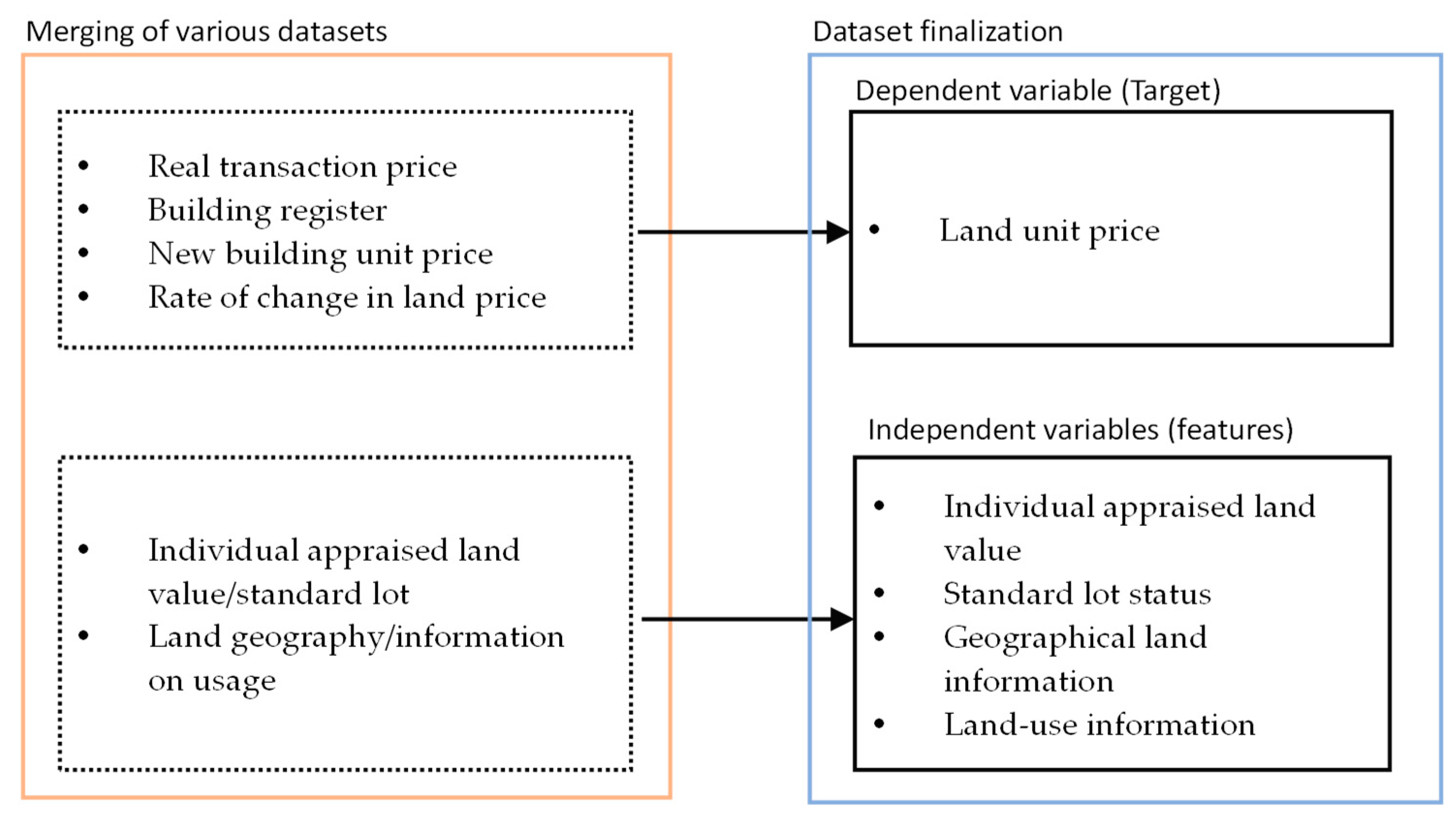
2.3. Variables
- Building price = Replacement cost − Depreciation amount (applied from the approved date of use to the transaction time);
- Land unit price at transaction time = (real transaction price of the real estate − Building price)/land area;
- Land unit price as of 31 December 2020 = land unit price at transaction time × rate of change in land price (from the transaction time to 31 December 2020).
2.4. Analysis
2.4.1. Analytical Framework
2.4.2. Machine Learning Methods: RF and XGBoost
2.4.3. Model Evaluation Measure
- Prediction is correct if
3. Results
3.1. Summary Statistics
3.2. Empirical Results: Prediction Modeling
4. Discussion
5. Conclusions
Author Contributions
Funding
Institutional Review Board Statement
Informed Consent Statement
Data Availability Statement
Conflicts of Interest
References
- McDonald, J.F.; McMillen, D.P. Urban Economics and Real Estate: Theory and Policy; John Wiley & Sons: Hoboken, NJ, USA, 2010. [Google Scholar]
- Wong, S.K.; Yiu, C.Y.; Chau, K.W. Liquidity and information asymmetry in the real estate market. J. Real Estate Financ. Econ. 2012, 45, 49–62. [Google Scholar] [CrossRef]
- Clayton, J. Further evidence on real estate market efficiency. J. Real Estate Res. 1998, 15, 41–57. [Google Scholar] [CrossRef]
- Kim, Y.; Choi, S.; Yi, M.Y. Applying comparable sales method to the automated estimation of real estate prices. Sustainability 2020, 12, 5679. [Google Scholar] [CrossRef]
- Hastie, T.; Tibshirani, R.; Friedman, J. The Elements of Statistical Learnin, 2nd ed.; Springer: Berlin/Heidelberg, Germany, 2009; p. 33. [Google Scholar]
- Simlai, P.E. Predicting owner-occupied housing values using machine learning: An empirical investigation of California census tracts data. J. Prop. Res. 2021, 1–32. [Google Scholar] [CrossRef]
- Schulz, R.; Wersing, M. Automated Valuation Services: A case study for Aberdeen in Scotland. J. Prop. Res. 2021, 154–172. [Google Scholar] [CrossRef]
- Mullainathan, S.; Spiess, J. Machine Learning: An Applied Econometric Approach. J. Econ. Perspect. 2017, 31, 87–106. [Google Scholar] [CrossRef] [Green Version]
- Čeh, M.; Kilibarda, M.; Lisec, A.; Bajat, B. Estimating the Performance of Random Forest versus Multiple Regression for Predicting Prices of the Apartments. ISPRS Int. J. Geo-Inf. 2018, 7, 168. [Google Scholar] [CrossRef] [Green Version]
- Singh, A.; Sharma, A.; Dubey, G. Big data analytics predicting real estate prices. Int. J. Syst. Assur. Eng. Manag. 2020, 11, 208–219. [Google Scholar] [CrossRef]
- Pai, P.-F.; Wang, W.-C. Using Machine Learning Models and Actual Transaction Data for Predicting Real Estate Prices. Appl. Sci. 2020, 10, 5832. [Google Scholar] [CrossRef]
- Park, B.; Bae, J.K. Using machine learning algorithms for housing price prediction: The case of Fairfax County, Virginia housing data. Expert Syst. Appl. 2015, 42, 2928–2934. [Google Scholar] [CrossRef]
- Antipov, E.A.; Pokryshevskaya, E.B. Mass appraisal of residential apartments: An application of Random forest for valuation and a CART-based approach for model diagnostics. Expert Syst. Appl. 2012, 39, 1772–1778. [Google Scholar] [CrossRef] [Green Version]
- Alfaro-Navarro, J.-L.; Cano, E.L.; Alfaro-Cortés, E.; García, N.; Gámez, M.; Larraz, B. A Fully Automated Adjustment of Ensemble Methods in Machine Learning for Modeling Complex Real Estate Systems. Complexity 2020, 2020, 5287263. [Google Scholar] [CrossRef]
- Ho, W.K.; Tang, B.-S.; Wong, S.W. Predicting property prices with machine learning algorithms. J. Prop. Res. 2021, 38, 48–70. [Google Scholar] [CrossRef]
- Truong, Q.; Nguyen, M.; Dang, H.; Mei, B. Housing Price Prediction via Improved Machine Learning Techniques. Procedia Comput. Sci. 2020, 174, 433–442. [Google Scholar] [CrossRef]
- Davis, M.A.; Heathcote, J. The price and quantity of residential land in the United States. J. Monet. Econ. 2007, 54, 2595–2620. [Google Scholar] [CrossRef] [Green Version]
- Davis, M.A.; Palumbo, M.G. The price of residential land in large US cities. J. Urban Econ. 2008, 63, 352–384. [Google Scholar] [CrossRef] [Green Version]
- Bostic, R.W.; Longhofer, S.D.; Redfearn, C.L. Land Leverage: Decomposing Home Price Dynamics. Real Estate Econ. 2007, 35, 183–208. [Google Scholar] [CrossRef]
- Won, J.; Lee, J.-S. Investigating How the Rents of Small Urban Houses are Determined: Using Spatial Hedonic Modeling for Urban Residential Housing in Seoul. Sustainability 2018, 10, 31. [Google Scholar] [CrossRef] [Green Version]
- Won, J.; Lee, C.; Li, W. Are Walkable Neighborhoods More Resilient to the Foreclosure Spillover Effects? J. Plan. Educ. Res. 2017, 38, 463–476. [Google Scholar] [CrossRef]
- O’sullivan, A. Urban Economics, 9th ed.; McGraw-Hill Education: New York, NY, USA, 2018; p. 464. [Google Scholar]
- Alonso, W. Location and Land Use. Toward a General Theory of Land Rent; Series: Publicatin of the Joint Center for Urban Studies; Harvard University Press: Cambridge, MA, USA, 1964. [Google Scholar]
- Heikkila, E.; Gordon, P.; I Kim, J.; Peiser, R.B.; Richardson, H.W.; Dale-Johnson, D. What Happened to the CBD-Distance Gradient?: Land Values in a Policentric City. Environ. Plan. A Econ. Space 1989, 21, 221–232. [Google Scholar] [CrossRef]
- Giuliano, G.; Gordon, P.; Pan, Q.; Park, J. Accessibility and Residential Land Values: Some Tests with New Measures. Urban Stud. 2010, 47, 3103–3130. [Google Scholar] [CrossRef] [Green Version]
- Haider, M.; Miller, E.J. Effects of Transportation Infrastructure and Location on Residential Real Estate Values: Application of Spatial Autoregressive Techniques. Transp. Res. Rec. 2000, 1722, 1–8. [Google Scholar] [CrossRef]
- Lee, W.; Kim, N.; Choi, Y.-H.; Kim, Y.S.; Lee, B.-D. Machine Learning based Prediction of The Value of Buildings. KSII Trans. Internet Inf. Syst. 2018, 12, 3966–3991. [Google Scholar] [CrossRef]
- Rokach, L. Ensemble-based classifiers. Artif. Intell. Rev. 2010, 33, 1–39. [Google Scholar] [CrossRef]
- Breiman, L. Bagging predictors. Mach. Learn. 1996, 24, 123–140. [Google Scholar] [CrossRef] [Green Version]
- James, G.; Witten, D.; Hastie, T.; Tibshirani, R. An Introduction to Statistical Learning, 2nd ed.; Springer: New York, NY, USA, 2021; Volume XV, p. 607. [Google Scholar]
- Breiman, L. Random forests. Mach. Learn. 2001, 45, 5–32. [Google Scholar] [CrossRef] [Green Version]
- Géron, A. Hands-On Machine Learning with Scikit-Learn, Keras, and TensorFlow: Concepts, Tools, and Techniques to Build Intelligent Systems; O’Reilly Media: Newton, MA, USA, 2019. [Google Scholar]
- He, H.-M.; Chen, Y.; Xiao, J.-Y.; Chen, X.-Q.; Lee, Z.-J. Data Analysis on the Influencing Factors of the Real Estate Price. Artif. Intell. Evol. 2021, 2021, 52–66. [Google Scholar] [CrossRef]
- Chen, T.; Guestrin, C. Xgboost: A scalable tree boosting system. In Proceedings of the 22nd ACM SIGKDD International Conference on Knowledge Discovery and Data Mining, San Francisco, CA, USA, 13–17 August 2016. [Google Scholar]
- Wade, C. Hands-On Gradient Boosting with XGBoost and Scikit-Learn; Packt Publishing Ltd.: Birmingham, UK, 2020; p. 310. [Google Scholar]
- Abidoye, B.R.; Chan, A.P.C. Improving property valuation accuracy: A comparison of hedonic pricing model and artificial neural network. Pac. Rim Prop. Res. J. 2018, 24, 71–83. [Google Scholar] [CrossRef]
- Crosby, N.; Lavers, A.; Murdoch, J. Property valuation variation and the ’margin of error’ in the UK. J. Prop. Res. 1998, 15, 305–330. [Google Scholar] [CrossRef]
- Watkins, C.A. The definition and identification of housing submarkets. Environ. Plan. A 2001, 33, 2235–2253. [Google Scholar] [CrossRef]
- Jones, C.; Leishman, C.; Watkins, C. Housing market processes, urban housing submarkets and planning policy. Town Plan. Rev. 2005, 76, 215–233. [Google Scholar] [CrossRef]
- Bramley, G. Land-use planning and the housing market in Britain: The impact on housebuilding and house prices. Environ. Plan. A 1993, 25, 1021–1051. [Google Scholar] [CrossRef]
- Valier, A. Who performs better? AVMs vs hedonic models. J. Prop. Investig. Financ. 2020, 38, 213–225. [Google Scholar] [CrossRef]


| Residential Areas | Commercial Areas | Industrial Areas | Green Areas | Total | |
|---|---|---|---|---|---|
| 2017 | 14,078 | 662 | 328 | 236 | 15,304 |
| 2018 | 12,448 | 784 | 312 | 256 | 13,800 |
| 2019 | 10,044 | 825 | 304 | 213 | 11,386 |
| 2020 | 11,085 | 823 | 283 | 219 | 12,410 |
| Total | 47,655 | 3094 | 1227 | 924 | 52,900 |
| Model | Python Library | Hyperparameter |
|---|---|---|
| Random Forest | RandomforestRegressor from Scikit-Learn | n_estimators = 10,000, max_depth = 9, and default for others (n_estimators = 100, criterion = ‘mse’, max_depth = None, min_samples_split = 2, min_samples_leaf = 1, min_weight_fraction_leaf = 0.0, max_features = ‘auto’, max_leaf_nodes = None, min_impurity_decrease = 0.0, min_impurity_split = None, bootstrap = True, oob_score = False, n_jobs = None, random_state = None, verbose = 0, warm_start = False, ccp_alpha = 0.0, max_samples = None) |
| XGBoost | XGBoostRegressor from Scikit-Learn Wrapper | n_estimators = 18,385, max_depth = 6, learning_rate = 0.005, obj = squarederror, and default for others (base_score = 0.5, booster = gb_tree, colsample_bylevel = 1, colsample_bynode = 1, colsample_bytree = 1, gamma = 0, importance_type = ‘gain’, max_delta_step = 0, min_child_weight = 1, missing = None, nthread = −1, reg_alpha = 0, reg_lambda = 1, scale_post_weight = 1, seed = 0, subsample = 1, verbosity = 1) |
| Variables | Descriptions | Mean/ Frequency | S.D. (Min.–Max.)/ % |
|---|---|---|---|
| Dependent variable (Target) | |||
| Land unit price | Continuous: (KRW) | 8,109,860 | 7,322,789 (9201–326,671,182) |
| Independent variables (Features) | |||
| Appraisal Information | |||
| Appraised land value | Continuous: (KRW) | 4,466,413 | 3,785,368 (7240–176,000,000) |
| Standard lot status | Binary: 1: standard lot | 2403 | 4.543% |
| 0: non-standard lot | 50,497 | 95.457% | |
| Geographical Land Information | |||
| Area | Continuous: m2 | 199.931 | 992.714 (3.3–177435) |
| Topography | Category: 1: Steep slope | 393 | 0.743% |
| 2: Undulating slope | 1275 | 2.410% | |
| 3: Flatland | 10,749 | 20.319% | |
| 4: Low-lying area | 38 | 0.072% | |
| 5: Elevated area | 40,445 | 76.456% | |
| Shape | Category: 1: Irregular | 4447 | 8.406% |
| 2: Square | 8577 | 16.214% | |
| 3: Ladder | 16,059 | 30.357% | |
| 4: Triangle | 828 | 1.565% | |
| 5: Flag | 3199 | 6.047% | |
| 6: Vertical rectangle | 13,620 | 25.747% | |
| 7: Horizontal rectangle | 6147 | 11.620% | |
| 8: Inverted triangle | 23 | 0.043% | |
| Abutting road | Category: 1: Thoroughfare | 3142 | 5.940% |
| 2: Medium-sized road | 3096 | 5.853% | |
| 3: Medium-narrow road | 6971 | 13.178% | |
| 4: Narrow road | 39,267 | 74.229% | |
| 5: Land with no road access | 424 | 0.802% | |
| Land Use Information | |||
| First main zoning | Category: 1: Residential | 47,655 | 90.085% |
| 2: Commercial | 3094 | 5.849% | |
| 3: Industrial | 1227 | 2.319% | |
| 4: Green | 924 | 1.747% | |
| Area of first main zoning | Category: 1: Residential | 163.830 | 211.528 (3.4–14,149) |
| 2: Commercial | 231.112 | 1037.090 (3.4–49,206) | |
| 3: Industrial | 241.188 | 543.344 (4–8209) | |
| 4: Green | 1687.738 | 6912.444 (5–177,435) | |
| Second main zoning | Category: 1: Residential | 793 | 1.499% |
| 2: Commercial | 61 | 0.115% | |
| 3: Green | 55 | 0.104% | |
| Area of second main zoning | Category: 1: Residential | 0.7658 | 15.649 (0–1920) |
| 2: Commercial | 13.710 | 91.575 (0–2630) | |
| 3: Industrial | 0.726 | 15.650 (0–478) | |
| 4: Green | 38.113 | 869.074 (0–2598) | |
| Restricted area | Binary: 1: Restricted area | 1372 | 2.594% |
| 0: Non-restricted area | 51,528 | 97.406% | |
| Specific use area | Binary: 1: Specific use area | 9623 | 18.191% |
| 0: Non-specific use area | 43,277 | 81.809% | |
| Forest land | Binary: 1: Forest land | 269 | 0.509% |
| 0: other than forest land | 52,631 | 99.491% | |
| Farmland | Binary: 1: farmland | 274 | 0.518% |
| 0: other than farmland | 52,626 | 99.482% | |
| Waste | Binary: 1: waste | 40,846 | 77.214% |
| 0: other than waste | 12,054 | 22.786% | |
| Planned facilities | Binary: 1: planned facilities | 3898 | 7.369% |
| 0: other than planned facilities | 49,002 | 92.631% | |
| Planned facility conflict rate | Continuous: % | 47.44 | 53.22 (0–100) |
| Land category | Category: 1: Park site | 4 | 0.008 |
| 2: Orchard | 4 | 0.008 | |
| 3: Rice paddy | 274 | 0.518 | |
| 4: Site | 51,518 | 97.388 | |
| 5: Forest land | 348 | 0.658 | |
| 6: Miscellaneous land | 90 | 0.170 | |
| 7: Factory site | 65 | 0.123 | |
| 8: Field (dry) | 451 | 0.853 | |
| 9: Site for religious use | 30 | 0.057 | |
| 10: Gas station land | 29 | 0.055 | |
| 11: Parking site | 30 | 0.057 | |
| 12: Storage site | 3 | 0.006 | |
| 13: Right of way | 31 | 0.059 | |
| 14: Site for athletics use | 1 | 0.002 | |
| 15: School site | 22 | 0.042 | |
| Distance to railway land | Category: 1. Within 10 m 2. Within 50 m 3. Within 100 m 4. Within 500 m 5. Beyond 500 m | 2443 4380 9953 17,861 18,263 | 4.62 8.28 18.81 33.76 34.52 |
| Land use details | Category: 1: Industrial | 256 | 0.484% |
| 2: Orchard | 5 | 0.009% | |
| 3: Residential | 37,004 | 69.951% | |
| 4: Commercial | 7519 | 14.214% | |
| 5: Farmland | 542 | 1.025% | |
| 6: Residential and commercial complex | 6781 | 12.819% | |
| 7: Office | 556 | 1.051% | |
| 8: Forest land | 237 | 0.448% | |
| Year | Data | RF | XGBoost | ||||
|---|---|---|---|---|---|---|---|
| M1 | M2 | M3 | M1 | M2 | M3 | ||
| 2017–2020 (N = 52,900) | Training | 76.46 | 45.30 | 78.39 | 85.91 | 55.09 | 88.96 |
| Test | 75.42 | 45.30 | 77.41 | 84.03 | 56.19 | 87.82 | |
| All | 75.98 | 45.98 | 77.93 | 83.46 | 53.99 | 86.50 | |
| 2020 (N = 12,410) | Training | 76.29 | 53.49 | 73.87 | 88.00 | 56.30 | 90.95 |
| Test | 73.81 | 51.78 | 76.67 | 84.51 | 55.98 | 90.44 | |
| All | 74.98 | 51.99 | 74.28 | 85.86 | 54.58 | 89.76 | |
| Year | Zones | Data | RF | XGBoost | ||||
|---|---|---|---|---|---|---|---|---|
| M1 | M2 | M3 | M1 | M2 | M3 | |||
| 2017–2020 | Residential (N = 47,655) | Training | 78.48 | 47.22 | 80.49 | 78.58 | 49.28 | 80.89 |
| Test | 76.57 | 45.66 | 78.04 | 75.92 | 45.74 | 78.70 | ||
| All | 77.44 | 46.30 | 78.55 | 76.19 | 47.94 | 79.29 | ||
| Commercial (N = 3094) | Training | 70.33 | 58.29 | 72.98 | 83.99 | 68.98 | 84.09 | |
| Test | 68.93 | 57.57 | 73.44 | 82.69 | 66.06 | 83.78 | ||
| All | 67.89 | 58.50 | 73.93 | 83.00 | 66.91 | 83.91 | ||
| Industrial (N = 1227) | Training | 77.84 | 62.99 | 76.83 | 86.04 | 73.91 | 87.95 | |
| Test | 75.80 | 60.70 | 77.56 | 84.98 | 71.09 | 85.38 | ||
| All | 76.84 | 61.98 | 76.84 | 85.98 | 72.98 | 86.90 | ||
| Green (N = 924) | Training | 59.30 | 57.30 | 61.98 | 83.98 | 75.99 | 85.09 | |
| Test | 58.00 | 55.97 | 63.33 | 81.56 | 73.45 | 83.58 | ||
| All | 58.30 | 56.49 | 62.69 | 82.99 | 74.99 | 84.99 | ||
| 2020 | Residential (N = 11,085) | Training | 77.49 | 55.48 | 79.39 | 85.91 | 55.98 | 86.09 |
| Test | 74.51 | 52.65 | 77.27 | 83.37 | 52.83 | 84.85 | ||
| All | 76.49 | 53.30 | 78.28 | 84.12 | 53.99 | 84.99 | ||
| Commercial (N = 823) | Training | 72.33 | 66.49 | 78.30 | 83.99 | 77.86 | 85.90 | |
| Test | 70.48 | 62.81 | 76.27 | 82.76 | 76.03 | 83.83 | ||
| All | 71.98 | 64.30 | 77.49 | 82.99 | 76.55 | 84.99 | ||
| Industrial (N = 283) | Training | 74.56 | 66.24 | 75.99 | 85.99 | 78.79 | 86.99 | |
| Test | 73.70 | 64.94 | 73.38 | 83.77 | 77.60 | 85.71 | ||
| All | 74.29 | 65.49 | 74.91 | 84.98 | 78.18 | 85.88 | ||
| Green (N = 219) | Training | 56.13 | 55.53 | 64.92 | 80.20 | 79.49 | 81.98 | |
| Test | 54.51 | 53.65 | 61.37 | 79.83 | 77.25 | 80.69 | ||
| All | 55.39 | 54.39 | 62.87 | 79.50 | 78.72 | 82.58 | ||
| Ranking | RF | XGBoost |
|---|---|---|
| 1 | Land appraisal value (0.160) | Land appraisal value (0.240) |
| 2 | Area (0.112) | Land use (0.153) |
| 3 | Main zoning area (0.107) | Dong (0.101) |
| 4 | Road condition (0.081) | Main zoning (0.087) |
| 5 | Land use (0.073) | Gu (0.049) |
| 6 | Dong (0.071) | Specific use district (0.041) |
| 7 | Main zoning (0.058) | Second zoning area (0.041) |
| 8 | Shape (0.058) | Second zoning (0.033) |
| 9 | Land category (0.058) | Road condition (0.031) |
| 10 | Bearing (0.039) | Accessibility to waste facilities (0.022) |
| 11 | Restrictions (0.034) | Restrictions (0.021) |
| 12 | Area ratio included (0.030) | Bearing (0.020) |
| 13 | Urban planning facilities (0.025) | Reference lot (0.017) |
| 14 | Accessibility to waste facilities (0.020) | Land category (0.016) |
| 15 | Agricultural land (0.020) | Area (0.015) |
| 16 | Distance to railway land (0.014) | Urban planning facilities (0.014) |
| 17 | Topography (0.013) | Main zoning area (0.014) |
| 18 | Reference lot (0.010) | Distance to railway land (0.014) |
| 19 | Specific-use district aea (0.006) | Year (0.013) |
| 20 | Forest land (0.004) | Area ratio included (0.013) |
| 21 | Second zoning (0.004) | Agricultural land (0.012) |
| 22 | Second zoning area (0.003) | Topography (0.011) |
| 23 | Gu (0.001) | Shape (0.011) |
| 24 | Year (0.001) | Forest land (0.010) |
Publisher’s Note: MDPI stays neutral with regard to jurisdictional claims in published maps and institutional affiliations. |
© 2021 by the authors. Licensee MDPI, Basel, Switzerland. This article is an open access article distributed under the terms and conditions of the Creative Commons Attribution (CC BY) license (https://creativecommons.org/licenses/by/4.0/).
Share and Cite
Kim, J.; Won, J.; Kim, H.; Heo, J. Machine-Learning-Based Prediction of Land Prices in Seoul, South Korea. Sustainability 2021, 13, 13088. https://doi.org/10.3390/su132313088
Kim J, Won J, Kim H, Heo J. Machine-Learning-Based Prediction of Land Prices in Seoul, South Korea. Sustainability. 2021; 13(23):13088. https://doi.org/10.3390/su132313088
Chicago/Turabian StyleKim, Jungsun, Jaewoong Won, Hyeongsoon Kim, and Joonghyeok Heo. 2021. "Machine-Learning-Based Prediction of Land Prices in Seoul, South Korea" Sustainability 13, no. 23: 13088. https://doi.org/10.3390/su132313088
APA StyleKim, J., Won, J., Kim, H., & Heo, J. (2021). Machine-Learning-Based Prediction of Land Prices in Seoul, South Korea. Sustainability, 13(23), 13088. https://doi.org/10.3390/su132313088