Abstract
This paper studies how policy interventions and economic factors affect COVID-19 infections and deaths, using generalized linear regression (GLM) models. We seek to explain the containment differences by countries’ inherent economic factors, especially the labor market structure, utilizing data from multiple sources. The results show that countries heavily relying on the service sector and international trade suffer more from the spreading, possibly due to the fact that COVID-19 is a communicable disease and spreads quickly through physical contact. Further, we find that these countries could benefit more from stringent policies compared to others.
JEL Classification:
I1-Health; O1-Economic Development
1. Introduction
The COVID-19 pandemic has caused significant public health, social, and global economic disruption with a rather fast spreading speed. However, it has transmitted at different rates in different parts of the world. Interestingly, we have witnessed counterintuitive facts that some countries, despite their existing economic and healthcare advantages, suffer more severely from the pandemic than others. To control the speed of spread, countries have undertaken a significant number of policy interventions such as lockdown, social distancing, quarantine, and use of masks since the beginning of the COVID-19 outbreak. Therefore, it is important for us to explore and understand the possible factors that affect the pandemic severity, not only in terms of policy interventions but also those factors from socio-economic perspectives that can inherently contribute to the spreading speed. These economic factors could also interact with the conducted policies and impact containment effectiveness. In this regard, this study explores both the direct and indirect effects of the economic factors on pandemic spreading speed, controlling for policy interventions and other related variables.
Socio-economic conditions add a significant amount of variability in the containment of any disease spread, especially, how that could inherently affect person-to-person contacts. Due to the nature of human-transmitted diseases, physical contacts create direct exposure to the viruses and naturally raise the risks of infection. People who are subject to significant numbers of physical contacts in their normal working schedules therefore will suffer higher exposure to virus transmissions. Several of the economic variables that catch our interest include the service sector percentages among all employment, international trade, and domestic savings percentages. These variables capture three aspects of different economies: labor market (employment) structure, reliance on international trade, and potential financial buffering.
We believe these economic factors that could significantly impact the degree of physical contact on the country level, and thus affect the pandemic spreading speed. First, employees in the service sectors will inevitably have more frequent physical contacts, and this higher than regular exposure could lead to faster than usual spread, especially without personal protection equipment (PPE). Second, frequent international trade could also lead to more infections because that allows the virus to transmit through international services or contaminated cargo surfaces. Studies suggest that COVID-19 survives on surfaces as well as in the air [1]. Some reports pointed out that it could survive for several days [2]. Third, the domestic savings will serve as a good financial buffer, and higher saving percentages of GDP should lead to lower spreading rates.
On the policy side, the stringency index can measure the impacts on direct contact frequencies; the economic support index can capture the financial buffering governments provide, which will enable people to sustain their everyday needs and stay at home even after unemployment shocks, this will, in turn, reduce the chances of contacts during the pandemic. Thus, greater measurements of these two indices should help reduce the infection as well as death rates.
We also adopt several other socio-economic-related factors as the control variables, including the percentage of population covered by safely managed sanitation, international tourism arrivals, area of the country, and percentage of the population living in urban areas that aggregate to more than one million.
COVID-19 case and death information were obtained from the Johns Hopkins University database. The dataset consists of 183 countries between 22 January 2020 to 15 November 2020, which covers 40 weeks of spreading observation periods. Country-specific socio-economic indicators are obtained from the World Development Indicators database documented by the World Bank. Policy variables, the stringency index, and the economic support index were obtained from the OxCGRT database at Oxford University.
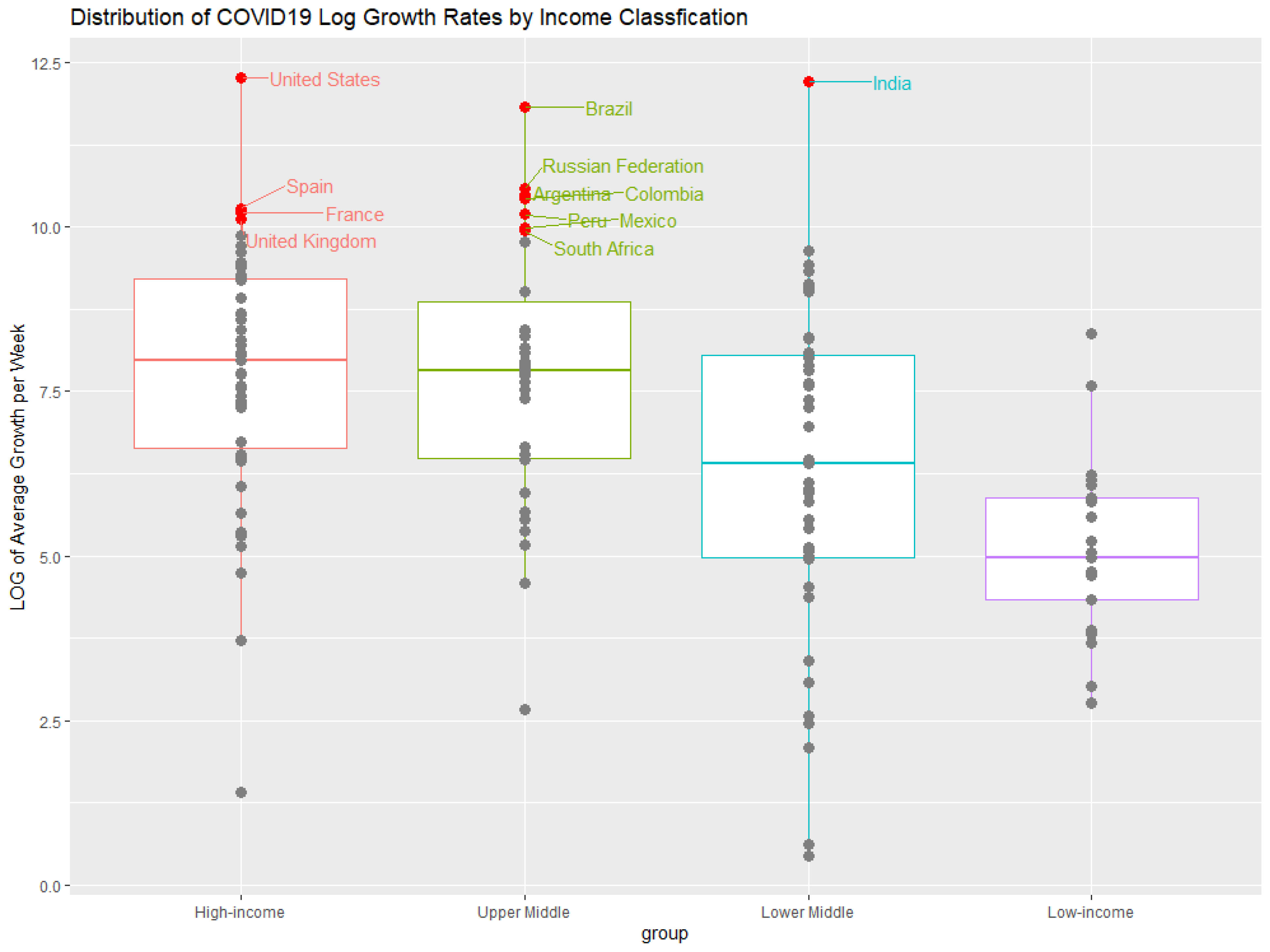
The motivation of this study comes from Figure 1. In the figure, it is noticeable that some countries (such as the United States, United Kingdom, Spain, France) have suffered from a higher average case growth rate per million population (displayed in natural logarithm term) than lower-income countries. This is counter-intuitive because developed nations are believed to have better healthcare systems and infrastructure facilities for sanitation services that are crucial to containing the disease quickly. In that context, this is the first study, to the best of our knowledge, that identifies various socio-economic factors that cause different COVID-19 spreading rates between countries with different economic advantages. These factors include, but are not limited to, the size of employment in service sectors, trade percentage of GDP, domestic saving percentage, and coverage of safely managed sanitation services, etc.
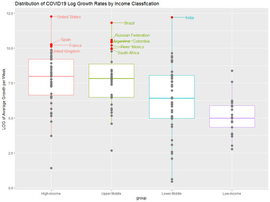
Figure 1.
Distribution of COVID-19 average growth rate by income classification.
Methodologically, we use the generalized linear regression models to analyze the data in order to investigate the relationship between the weekly case and death growth rates and country-specific characteristics. To take population into account, when we study the spreading patterns, the case growth and death rates are standardized per million population. Namely, to measure the severity of the pandemic, we use weekly case growth per million population, and weekly death growth rate per million population.
The results show that the case and death growth rates of COVID-19 spread are positively associated with the percentage of service-sector employment in a given country. The percentage of international trade to GDP is also positively associated with the growth rates. In addition, both domestic saving percentages and safely managed sanitation coverages have negative impacts on the speed of growth. The results indicate that the more likelihood of extended personal contacts and interactions are involved, the higher the growth rate of COVID-19 cases is expected. Our results do suggest that countries heavily relying on service-sector employment can benefit more from the stringent policies than those with less service involvement.
This study provides an insight into the factors that the governments can consider for an additional look as the potential contributors to the spread of the disease, inferring possible populations that are vulnerable to the disease due to social and economic structures, even economically and medically advanced areas. The policy implications of our study also suggest ensuring sanitation facilities to the general public, and in the meantime, paying extra attention to people who work in service sectors.
This study contributes to the literature in four ways: first, we seek to differentiate COVID-19 spreading among countries with different characteristics, to explain the containment differences by the inherent factors in their economic structure. Second, benefiting from longer observation periods, we are able to take advantage of the weekly data (instead of daily data) to generate better estimates by alleviating the issues from measurement errors, and delayed reports. We are also able to explore the impact of economic factors and policies by constructing the analysis based on different time periods so that to demonstrate the effects in the immediate short term, short term, or long term. Third, we investigate the effectiveness of policy interventions and their interactions with the existing economic structures within different time periods. Finally, this study also contributes to sustainable development. It is directly related to one of the seventeen goals of sustainable development, which is “good health and well-being”. Controlling the spread of COVID-19 could assist in promoting the health and well-being of people in different countries in the world. The findings of this study can be used to formulate more targeted policies and deploy the available resources for the future occurrence of a similar pandemic.
2. Motivation and Literature Review
The extent to which COVID-19 tolls vary by country is dependant on the overall effectiveness of countries’ policies towards COVID-19 management. In the different time periods of the COVID-19 outbreak, countries have applied various policies to control COVID-19 infections and mortality. To track such policies, ref. [3] developed the Oxford COVID-19 Government Response Tracker (OxCGRT). This provides a standardized methodology to assess the various government policies on COVID-19. It systematically collects information on several different common policy responses that governments have taken to respond to the pandemic on 18 indicators such as school closures and travel restrictions and covers more than 180 countries. We only focus on two of the indices, the stringency index and the economic support index. The stringency index includes school closures, workplace closing, cancelled public events, restrictions on gatherings, public transportation, stay at home orders, restrictions on internal movement, international travel controls, and public information campaigns. The economic support index covers income support and debt/contract relief for households.
The COVID-19 spread illustrates the role of mass gatherings in the exacerbation of the scope of pandemics. Cancellation or suspension of mass gatherings would be critical to pandemic mitigation [4]. However, it is more difficult to adopt these policies when the nature of employment is such that large gatherings cannot be easily avoided. In particular, the domination of the industrialized economies by service sectors adds more to this problem [5]. Welsch [6] examines the relationship between mask usage and COVID-19 deaths at the county level in the US and finds that a one percentage point increase in the number of individuals who wear a mask when within six feet of people will reduce COVID-19 deaths in a county by 10.5 percent on average.
However, there are some inherent socio-economic characteristics in the country that accelerate COVID-19 cases and deaths. Since it is a communicable disease, the spreading of COVID-19 is directly associated with human contact frequencies. For instance, urban areas are highly populated, and as a result, the likelihood of getting COVID-19 in such areas is high. Similarly, people in regions with a large flow of trade and with more people employed in service sectors would also have a higher chance of getting infected from this disease. Other factors that influence COVID-19 transmission rates could be the size of the aging population, people with chronic diseases or other underlying conditions, and access to basic sanitation services [7,8].
With a large COVID-related literature, the existing research on the impact of socio-economic status on COVID-19 cases and death, however, is limited. Using a panel dataset from 80 countries up to May 2020, ref. [9] finds that socio-economic circumstances have a strong negative association with COVID-19 confirmed daily cases and deaths. Additionally, the paper finds that social distancing measures policy and generous income support programs help lower the cases and deaths in countries with poor socio-economic conditions. Ashraf used a similar dataset to this paper; however, our focuses are different. For one thing, we are focusing on the socio-economic factors to explain the distinctive facts of spreading across 180 countries, while controlling for the different policies. Second, our paper uses weekly data up till November 2020 to handle the potential measurement errors and unnecessary daily fluctuations. Third, we provide comparisons of analysis across different time periods to demonstrate the effects of policies in the short term vs. long term. Other differences include the selection of variables, policies, and interaction terms.
Using the data on daily infection cases at the county level in the US, [10] finds that population density is associated with higher rates of COVID-19 transmission. This paper also suggests that there is a significant role of urban characteristics such as public transportation and local incomes in the speed of transmission. Ref. [11] study the spread of COVID-19 at the county level for the United States using data from the US Census Bureau and find that the prevalence of the disease and the death rate are correlated with the local socio-economic conditions.
According to [12], regardless of the lockdown, the number of COVID-19 cases in India increased by 80 percent. Furthermore, there was a differential impact across states, depending on the extent of healthcare facilities and preparedness [12,13,14]. This suggests that COVID-19 focused public policies may not work equally in all countries, and we can conclude that country-level underlying characteristics also play a vital role in the speed of spreading.
Developing countries generally have a younger population on average whereas developed countries have older ones. The relatively bigger size of younger people in developing countries gives them an advantage in facing the disease since the COVID-19 has the harshest impact on the elderly. On the other hand, developing countries have a lower quality of healthcare and less access to clean drinking water and sanitation [15], which leads to easy exposure to this disease.
Researchers have also explored the causes of death rates from this disease. For instance, ref. [16] suggests that the outcomes of this disease in developed countries may not be generalizable to developing countries, and a greater share of reported COVID-19 deaths occurs at younger ages in low- and middle-income countries compared to high-income countries. [17] suggest that the share of COVID-19 deaths in developed countries may increase sharply as the pandemic matures.
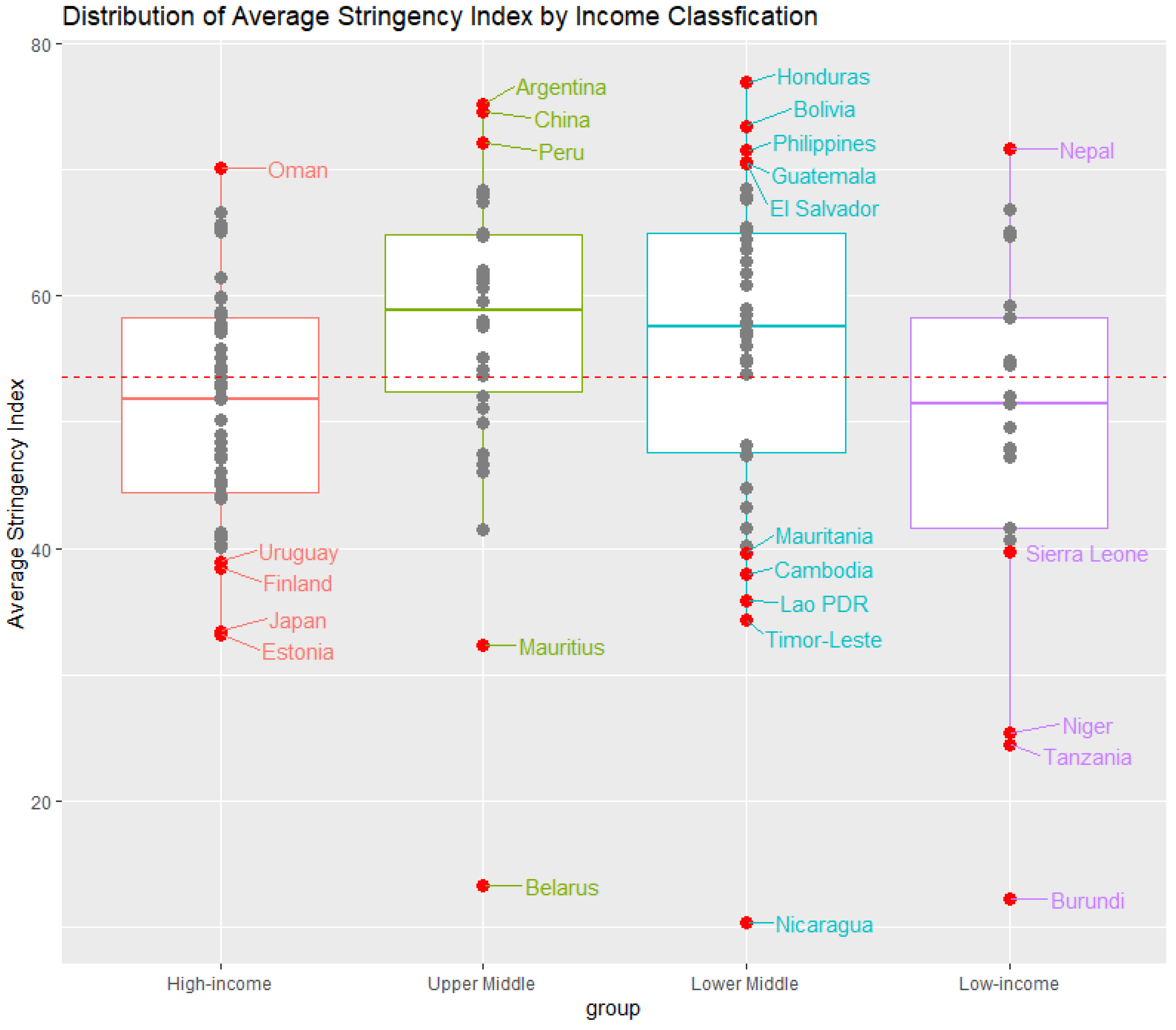
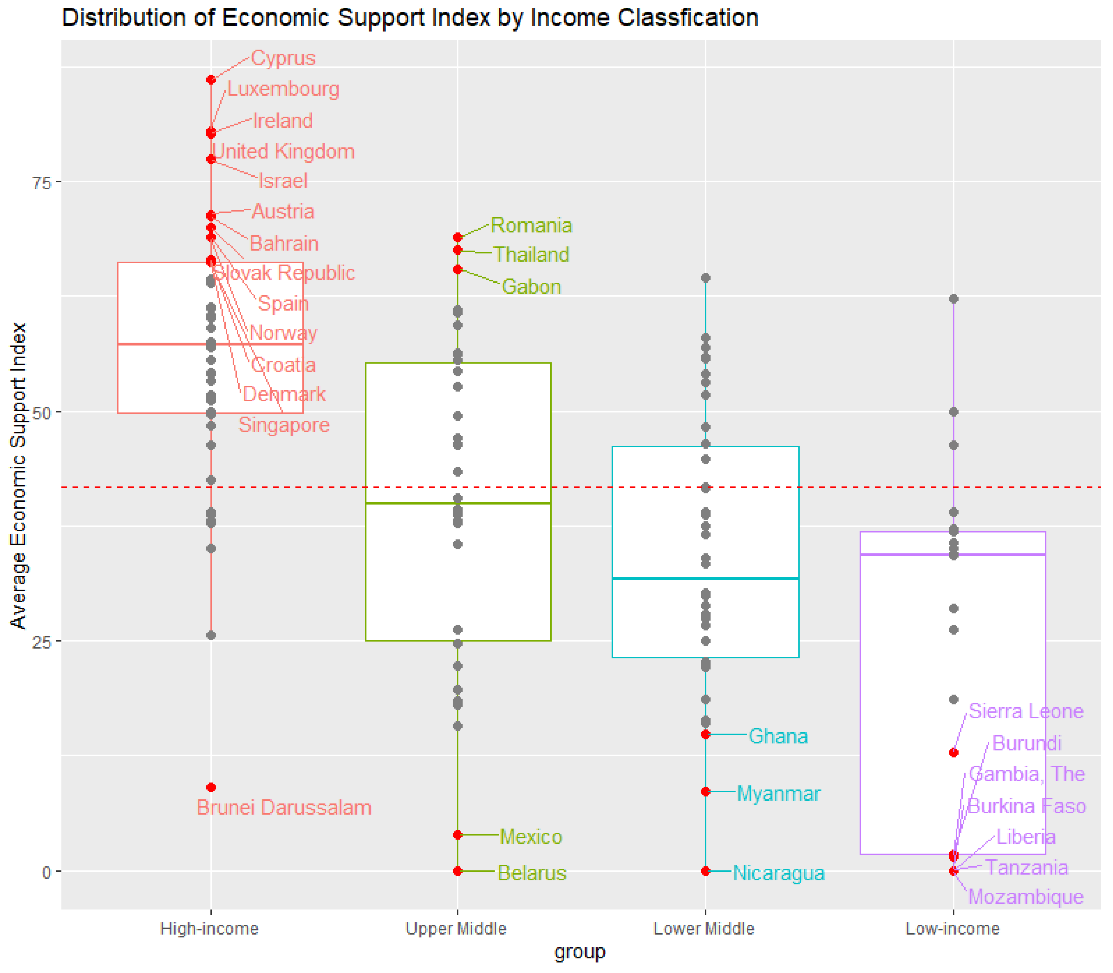
We present the policy indicators from OxCGRT by income classifications. Referring to Figure 2 and Figure 3, we have plotted the average stringency index and economic support index by country income groups. The four groups are high-income, upper-middle, lower-middle, and low-income groups. The stringency index does not demonstrate a clear difference between the different groups; however, the economics support index does reveal the trend that countries with economic advantages tend to provide higher economic support overall than those other counterparts. The similarities in the stringency index could be explained that most countries follow World Health Organization (WHO) advice in shutdowns or restrictions during the pandemic period, the consistent trends therefore would provide reasonably identical stringency. In the meantime, countries with economic advantages are able to provide reasonable economic support. Since there are no dramatic distinctions in the average policy measurements, but vast differences in case growth and death, we, therefore, want to explore the effects of policy interventions in different countries and different time periods in explaining the differentiated outcomes in disease control. We believe that stringency policy is expected to have a direct negative impact on the prevalence of COVID-19, through limiting physical contact and in turn reducing infections and deaths. On the other hand, Economic Support Policy is aimed to provide financial buffering during the pandemic, and it could provide an indirect effect on death rates by affording better healthcare. In the meantime, even with the same level of restriction or economic support, different countries might get impacted differently through the targeted policy interventions, due to different country-specific socio-economic characteristics. For instance, countries with economic disadvantages may benefit more from the same level of economic support compared to their counterparts. Therefore, we propose our first and second testable hypotheses as follows:
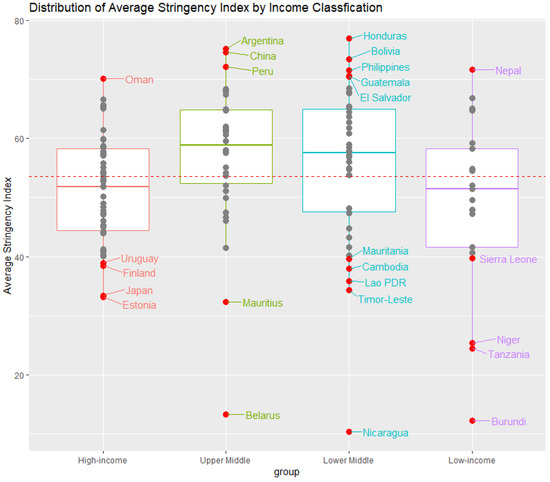
Figure 2.
Distribution of average stringency index by income classification.
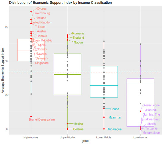
Figure 3.
Distribution of average economic support index by income classification.
Hypothesis 1 (H1).
The stringency index and economic support index are negatively associated with COVID-19 case growth and death rates.
Hypothesis 2 (H2).
Countries with different socio-economic statuses benefit from the stringency index and economic support index differently in alleviating COVID-19 case growth and death rates.
In general, policy intervention is subject to both administrative and operational delay, and it takes time before the policy creates a noticeable impact. Due to the lagged nature of policy effects, we are also interested in exploring the impacts along different time span. Therefore, it leads us to test the following hypothesis:
Hypothesis 3 (H3).
The impact of the stringency index and economic support index policies varies over time.
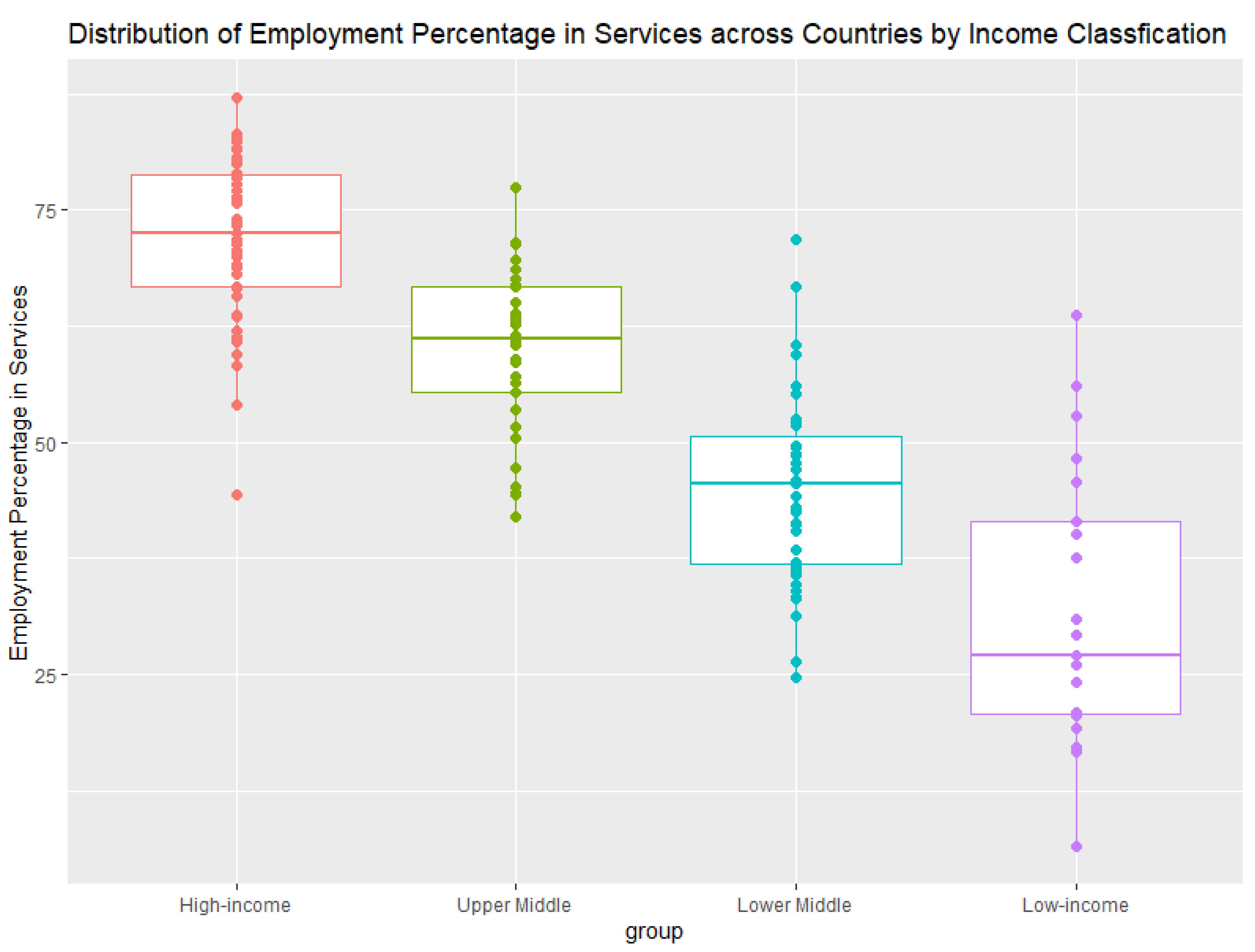
We present various socio-economic indicators that help explain the differences in factors that may influence the spread. We are most interested in the role that labor market structure plays, where the employment percentage in the service sector serves as a proxy. The service sector requires more frequent physical contact among people than other sectors, this makes the employees in the service sector more vulnerable to the pandemic. Figure 4 shows employment percentages in service sectors across different countries, and we see quite distinctive weights of the service sector among them. Based on this logic, countries with different dependencies on service sectors could get impacted differently from COVID-19. We suggest that larger dependency on the service sector could contribute positively to infection numbers, at least in the short run when the pandemic outbreaks. Thus, we propose our fourth hypothesis as:
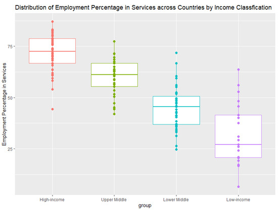
Figure 4.
Distribution of employment percentage in services by income classification.
Hypothesis 4 (H4).
A larger employment percentage in service sectors is positively associated with COVID-19 case growth and death rates.
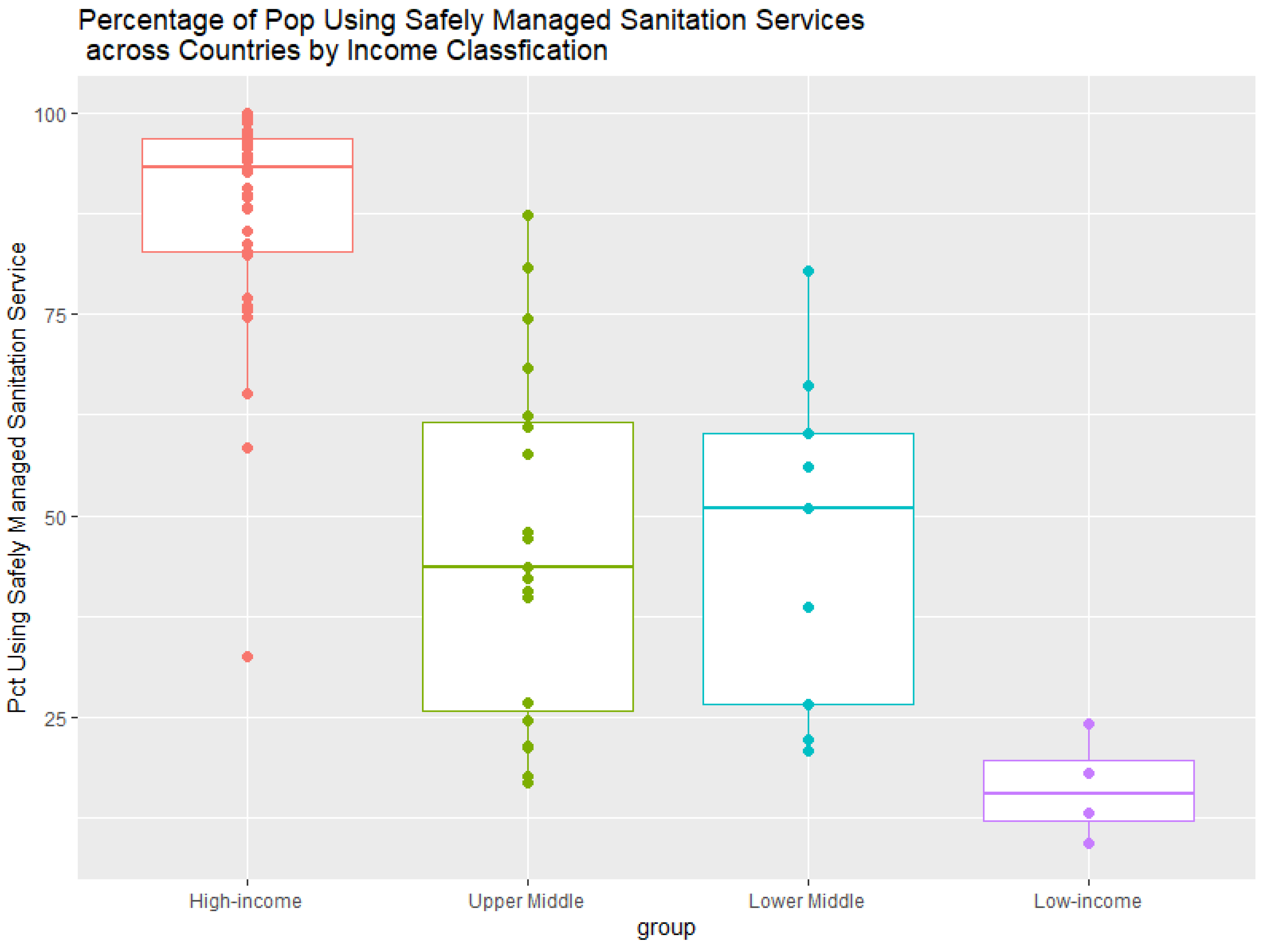
Other factors that naturally increase physical contact frequencies would also be closely linked to the spread of COVID-19. These factors include, for instance, the dependency of international trade, and population density. In addition, sanitation level is directly related to the protection level for communicable disease, and we expect that higher percentage coverage of the sanitation service to be negatively associated with COVID-19 case and death growth. These socio-economic factors used in our study are treated as control variables.
Figure 5 provides the percentage of international trade to GDP. Similarly, we can see that such a share is bigger in high-income countries than their counterparts. Figure 6 shows the percentage of the population covered with safely managed sanitation services by income classifications. It shows that countries with economic advantages have higher coverage than those countries with lower income.
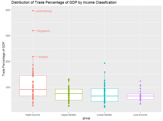
Figure 5.
International trade share of GDP by income classification.
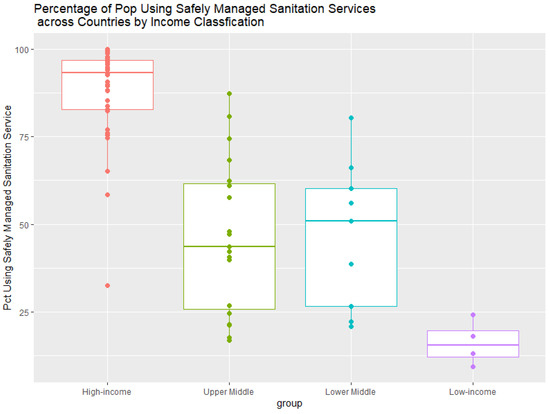
Figure 6.
Distribution of sanitation service coverage by income classification.
Referring to Figure 4, Figure 5 and Figure 6, the process of economic development provides a trend of expansion in service sectors, promoting and forcing more frequent physical contacts and interactions. The economic attractiveness of the developed countries further promotes international trade. By nature, COVID-19 is a type of communicable disease, so the population crowd will intuitively be positively correlated with the spreading speed of the disease. Our key point here is not that developed countries are at a disadvantage of this disease because they averaged with higher income, but the fact that countries with higher levels of economic development may be vulnerable to COVID-19 due to the increasing physical contacts and interactions due to their economic structure. Countries with economic disadvantages would still suffer from high infection rates as long as the pattern of economic development encourages more contacts, such as higher service sector percentages and higher international trade dependency. For example, Brazil and India both stand out in the average growth rate, demonstrated by Figure 1.
3. Methodology and Data
In this study, we have collected data from multiple sources. The COVID-19 data is obtained from Johns Hopkins University’s CSSE COVID-19 Dataset at GitHub (https://github.com/CSSEGISandData/COVID-19/tree/master/csse_covid_19_data, accessed on 22 November 2020). For our research purposes, the time series summary is used for the global confirmed cases. In total, we have weekly information for 183 countries or areas, from 22 January to 15 November 2020.
Country-specific attributes are obtained from the World Development Indicators (WDI) database, which is the World Bank’s premier compilation of cross-country data on development. The database contains annual information on GDP per capita, GNP per capita, employment percentages in different sectors, international trade volume, sanitation levels, population, etc. We have utilized the variables’ three-year averages to construct our measurement in socio-economic status. In addition, the World Bank assigns the world’s economies into four income groups—low, lower-middle, upper-middle, and high-income countries. The classifications are updated each year on July 1 and are based on GNI per capita in the current USD, using the Atlas method exchange rate. Our categorization of the world’s economies by income is based on GNI per capita cutoff values of 1025, 3395, and 12,375 respectively.
In addition, we have obtained policy-related data collected by the Blavatnik School of Government at the University of Oxford. The groups of indices provided by the OxCGRT database record the number and strictness of government policies, and are varying over time. Specifically, we focused on two indices that emphasized two different aspects of government policy, the stringency index and the economic support index.
The data statistics in Table 1, including the weekly case information from Johns Hopkins University, OxCGRT, and the country attributes from WDI.

Table 1.
Summary statistics.
In Appendix A, Figure A1 presents the cumulative COVID-19 cases by week across countries, and those nations with quite concerning trends are marked out with labels. Similarly, the graph depicting cumulative death cases by week is provided in an identical fashion in Figure A2. Table A1 displays the variable definitions from the WDI database, which are used in our regression analysis.
Our regression model is based on the time series of the global case data, seeking to identify the relationship between the weekly growth of COVID-19 cases and death numbers and country-specific characteristics so as to shed light on the reasons why some countries have better control of the pandemic spreading. We define the weekly change normalized by population size as our main variable of interest, growth rate, both for infection and death.
The conceptual framework is displayed as follows:
For country i, on week t, the observed COVID-19 growth (death) rates depend on the lagged cumulative cases in that country, social and economic status of interest, country-specific attributes as control variables, and the time-dependent disturbance term. are J numbers of the variables of interest for each country i, which include the percentage of employment in service sectors, trade percentage of GDP, percentage of the population with safely managed sanitation services, and GDP per capita. are the M numbers of country-specific control variables, including gross domestic savings as a percentage of GDP, tourism inflows (captured by the annual numbers of international tourism arrivals), geographic area of each country i, and percentage of the population in urban areas that aggregated more than 1 million people. We have also included the time fixed-effect term in our models, which is the time dummy, and it will be discussed in the result sections. To consider the impact of policies on the spreading trend through socio-economic factors, we include interaction terms of stringency policy and economic support policy with employment percentage in the service sector and GDP per capita. Since we started our work from a question of spreading between developed and developing countries, the GDP per capita can serve as a reasonable control, and the employment percentage in the service sector can capture the labor market structures, which reveals physical contact involvement among the workers.
For simplicity of explanation, we denote the normalized weekly cases and death changes as growth rates, since they are measuring the changing rates in consecutive weeks. Both variables are calculated based on the cumulative cases, and defined in the following two ways as described in Equations (2) and (3):
The COVID-19 case growth rate (CPM), is the weekly increase of COVID-19 cases per million of the population for one specific country i. The design of our growth rates is aimed to capture the case change ratios (severity of the spread) along with each country so that to provide stable indices that can be used to track the trend of COVID-19. Since the case measurement across weekdays and weekends may not be consistent, we believe the weekly aggregation will suffer less from measurement errors of daily fluctuations, and would in turn serve better to reveal the actual trend of case growth. Further, the COVID-19 death growth rate (DPM), is the weekly increase of death per million of population. The design also takes into account the population size of each country, so as to reveal the severity of the pandemic. An alternative way to capture the COVID-19 trend, other than the growth rates that we use, is the ratio of case change of a specific day over the cumulative cases up to that day. However, this alternative variable generally has a downward trend and drops quickly if the cumulative cases rise fast enough, this makes the variable fail to capture the trend of interest (in the case of the United States, the quick increase in cumulative cases makes this alternative variable approach zero, even when the daily increments of COVID-19 cases are as high as 20,000).
Based on the nature of unbalanced panels, and the fact that country-specific attributes (GDP per capita, country area, etc.) are available in the annual format from the World Bank database, the only dynamics we have in the timely fashion is the variations in weekly case numbers and policy changes. Thus, we proceeded with generalized linear regressions using the “PLM” package from R, and estimated the coefficients through the maximum likelihood method using the time fixed-effect model. Our identification strategy is to utilize the time-lagged term as explanatory variables (including government policies, infection numbers, and historical country-specific characters) so that to resolve concerns on the potential endogeneity issues. Hence, we believe our models are correctly identified.
4. Results
This section presents results that investigate the relationship between country-level socio-economic factors and the growth rate of COVID-19 cases. Table 2 demonstrates the regression results showing the correlation between the growth rate of COVID-19 cases and the economic status of a specific country. Here, the reference group is developing country groups (which include upper-middle, lower-middle-income countries, as well as low-income countries). The results show that in general, developed countries have higher growth rates compared to those developing countries, and the result is robust across different time periods. For instance, the coefficients of developed country groups on case growth rates are statistically significant at a 1 percent level. This is the starting point of our research—we seek to explain the counterintuitive fact that developed countries, despite the advantages they have in many aspects, are actually quite vulnerable to the COVID-19 pandemic due to the fact that it is a communicable disease and will spread quickly through contacts and interactions.
Table 2.
COVID-19 case growth rates—developed vs. developing countries.
Table 3 follows the same fashion as in Table 2, we are providing a more detailed categorization of the countries by the World Bank GNI standard. Here, the base group is the low-income country group. Identically, we have used the time fixed-effect model. To visualize, we have also provided plots on case growth rates in Figure 1. The graph shows the comparisons between some representative countries with the highest level of case growth rates (normalized by population size) along with income classifications. We have also pinpointed the outlier countries (with unusually high infections) for references. The results show that countries with relatively higher income levels have higher growth rates compared to the low-income country groups. For example, compared to low-income countries, the average growth rates of high-income and upper-middle-income countries are significantly higher, across different types of growth rate measurements and models. The results are statistically significant at 1 percent level, and quite consistent across different categories of income levels. This leads us to further explore the specific attributes these countries (who have better economic advantages) have.
Table 3.
COVID-19 case growth rate by income categories.
Table 4 and Table 5 demonstrate the main results of this paper. We have provided two types of COVID tracking indexes including case growth rate and death growth rate, both defined as per million of the population to reveal the time trend of increments. Specifically, we categorized the spreading of COVID-19 by intervals of 10 weeks, and seek to explore the effect of different social-economic factors in influencing the spreading or mortality of the disease. We estimated model coefficients using time fixed-effect models, through maximum likelihood estimation. Each column demonstrates regression results within a specific time period, the first ten weeks, the first twenty weeks, etc. The values displayed without parentheses are the estimated coefficients, and values in the parenthesis are standard errors. Our main interest is the role socio-economic status plays in the pandemic; therefore, we have utilized the data from the World Bank in characterizing different economies. One of our major focuses is the percentage of employment in the service sector, since a larger proportion of employment in services contributes positively towards personal interactions, and thus could lead to faster spreading of the disease. Furthermore, countries heavily involved in international trade will naturally have more personal interactions and contacts and therefore could lead to faster spread. Last but not least, the percentage coverage of safely managed sanitation services reveals the differentiations among countries as the sanitation availability background. Intuitively, nations with higher coverage in these services should help reduce the spreading speed. In the meantime, we are also interested in the effects of government policies and the interaction of socio-economic factors with the policies. We focus on two policies: the stringency policy index covers the restriction imposed by governments on closures/shutdowns, as well as in the public information disclosures/announcements; the economic support index covers the financial relief that governments are providing. According to the regression results, the percentage of employment in the service sector contributes positively across different time periods. Higher international trade percentage of GDP is positively related to the spreading, this seems to be intuitive since countries relying heavily on imports and exports tend to have a higher frequency of interactions and contacts, which would, in turn, accelerate the spreading of the disease. Coverage of sanitation services contributes consistently negatively to the spreading, demonstrating the benefit of wide coverage in safely managed sanitation.
Table 4.
Regression analysis on death growth rates.
Table 5.
Regression analysis on case growth rates.
On the other hand, the effects of government policies differ. The stringency policy has provided a significant reduction in case growth rate along the different time periods during the pandemic. The economic support policy, measured by the economic support index, does contribute negatively to the growth rates, however, are weakly significant and only in the early periods. The effect of the economic support index is not statistically significant in the immediate short run, possibly due to the feasible unemployment benefits that people can secure, and the effects fade away once we are looking at relatively long-term periods.
Each percentage point increase in the service sector employment will increase the weekly infection by about 4 percent in the fixed-effect models. Each unit increase in the stringency index (two period lagged) helps reduce 10 percent infection (case per million population), and each unit increase in economic support index (two period lagged) helps reduce about 3 percent in case growth rates.
To explore the effect of employment percentage in service through different policies, we interact policies with the service percentages. The results show that the coefficients on the interaction term are significantly negative at the 5 percent level, meaning that countries with a larger proportion of the service sector will benefit more from the stringency policies. However, we do not find evidence of consistently significant results on the effect of employment percentage in service through economic support policies. These results provide policy implications to encourage countries with higher percentages of labor force employing in the service sector (countries that rely heavily on service sectors) to adopt restrictive policies in mitigating the pandemic. Additionally, it is also quite intuitive that economic support, such as sending out stimulus checks, could help strengthen population confidence and follow restrictive orders (without worrying about income) in the fairly short run. Since the government cannot provide consecutive economic support to individuals, this type of policy would not be effective in the relatively long term.
We also include other variables to serve as controls, including savings percentages of GDP, countries’ geographic area (km squares), international tourism arrivals, and population in urban areas that aggregate for more than 1 million. We have found that the savings percentage of GDP has a negative significant effect on the case growth rate, suggesting that countries would benefit from higher levels of savings, possibly due to the financial buffering effect. Additionally, the geographic areas have negative effects on the growth rate (per million population), which could be explained that larger geographic areas provide less person-to-person contacts and interactions, and thus help reduce the spreading. The empirical evidence shows that countries with a higher frequency of interactions (higher employment percentage in service, higher trade percentages, etc.) could face faster spreading due to their existing economic structures as a result, while those with better sanitation coverages have an advantage in handling the spreading.
Table 4 provides regression results of death growth rate, measured as death weekly increase per million population, and delivers quite consistent results as in Table 5 for case growth rates. Here the stringency policy’s effect to reduce death is still statistically significant especially when we focus on the long term. The economic support policy, on the other hand, provides long-lasting effects, possibly because of the lagged nature of death following infection. Even if the economic support may not help people reduce chances of infection, the effects will be delivered through better healthcare after the diagnosis of infection, and eventually, help reduce death cases. The employment percentage in the service sector again reveals positive and significant effects on death growth rates. The negative signs on the interaction term of employment in the service sector still demonstrate the fact that countries with a higher proportion of employment in services would benefit more from higher stringency (more restricted policies) than those countries with less service employment. Again, we included variables like GDP per capita, trade percentages, savings percentages, safely managed sanitation coverage, geographic areas, international tourism arrivals, and the percentage of the population in urban areas that aggregate for more than 1 million. The results are in general robust compared to our regressions of case growth rate.
5. Discussion and Conclusions
This study identifies various socio-economic factors that could contribute to the COVID-19 spread. To identify such factors, we use Johns Hopkins University’s COVID-19 Dataset, OxCGRT database of government response, and World Development Indicators (WDI) from the World Bank. Empirically, we use generalized linear regression models and estimated the coefficients using the maximum likelihood methods. Our results show that economic structures play an important role. For instance, the percentage of employment in service sectors, and international trade percentages are positively associated with the growth and death rates in COVID-19 cases. On the other hand, the domestic saving percentages and percentage of population covered by safely managed sanitation services are negatively associated with the spreading. In the meantime, both stringency policies and economic support policies have effects in alleviating the spreading speed and death rates. The overall trend of employment transformation along economic growth leads to expansions in service sectors. Despite the economic prosperity that the service sector brings, this type of employment structure forces more physical contact involvement, and therefore would make these countries more vulnerable under the current kind of communicable disease pandemic, at least in the short run. However, our results do suggest that countries heavily relying on service-sector employment can benefit more from the stringent policies than those with less service involvement. One of the central issues in the current sustainability debate is the balancing of economic development and social considerations. There might be a trade-off between economic and social dimensions of sustainable development because of the availability of resources. On one hand, economic development focuses on productivity, efficiency, investment, employment, trade openness, etc. On the other hand, social considerations are related to accessibility, affordability, disparities, and safety. To achieve sustainable development, we need to balance these two dimensions. If one dimension is weak, the propensity of controlling infectious diseases such as COVID-19 would decrease, in turn, it negatively impacts the sustainability goals.
Similarly, the role of institutions, both the formal and informal, in shaping economic as well as social behavior is crucial. The rules, norms, values, policies, routines, etc., influence the behavior of people in societies. As a result, strong institutions may cause to reduce the spread of infectious diseases including COVID-19.
This study provides an insight into the factors that the governments can consider for an additional look as the potential contributors to the spread of the disease, inferring possible populations that are vulnerable to the disease due to social and economic structures, even economically and medically advanced areas. The policy implications of our study suggest ensuring sanitation facilities to the general public, and in the meantime, pay extra attention to people who work in service sectors, and those without enough coverage of safely managed sanitation services.
However, this paper has some caveats. There are some other potential factors in the public health literature that could make people vulnerable to COVID-19, including the size of the aging population, preconditions of chronic disease, past surgery histories, other cardiovascular diseases, etc. These are not our main focus and will not be discussed here. Additionally, the number of confirmed cases would be dependent on the number of tests given and the general availability of testing. Therefore, it is possible that the changes in the infection and death rate in the paper might be driven by cross-country differences in testing capacities. If the country has inadequate or low testing levels, both the infection and death cases may also be underreported, making them less representative indicators. Next, due to data limitations on the test-availability data, we use the observed case numbers to proxy the actual cases. We believe this will not significantly bias our results because this study focuses on the COVID-19 trend from a relatively long-term perspective. Lastly, the COVID-19 death classification could be different among different countries, induced by either technological, medical, or sometimes even political reasons. Again, we assume the reported death counts can serve as a good approximation of the actual deaths due to COVID-19, at least in the relatively long run.
Author Contributions
Both authors, Y.L. and K.P.K., equally contributed in all sections of the paper. All authors have read and agreed to the published version of the manuscript.
Funding
This research received no external funding.
Institutional Review Board Statement
Not applicable.
Informed Consent Statement
Not applicable.
Data Availability Statement
Data is not publicly available, though the data may be made available on request from the corresponding author.
Conflicts of Interest
The authors declare no conflict of interest.
Appendix A
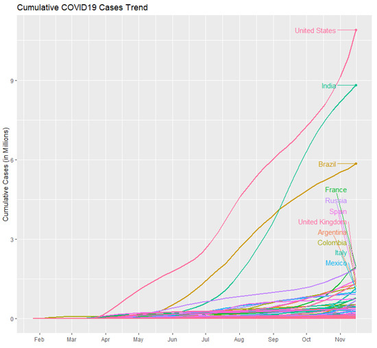
Figure A1.
Cumulative COVID-19 case numbers time trend.
Figure A1.
Cumulative COVID-19 case numbers time trend.
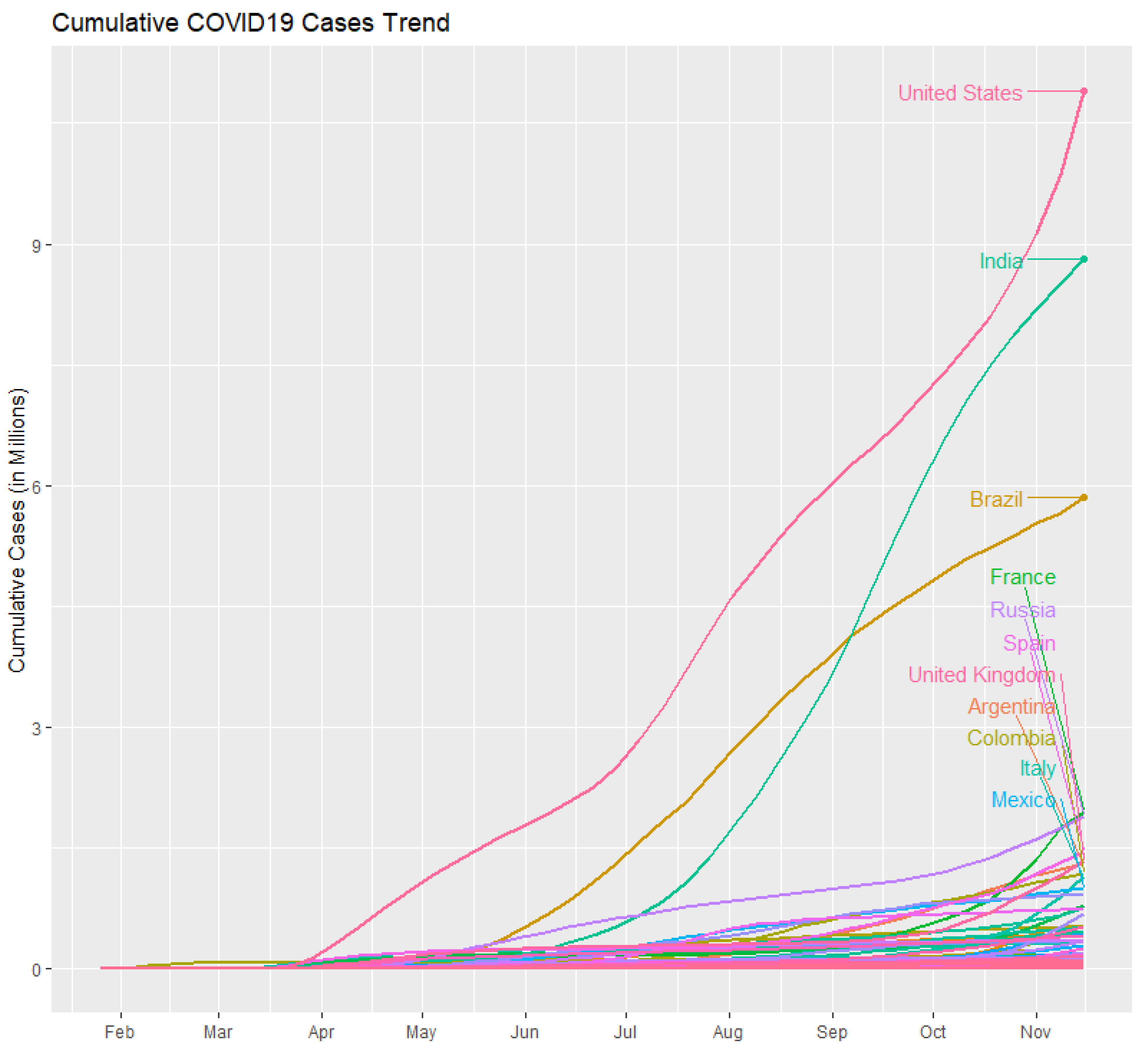
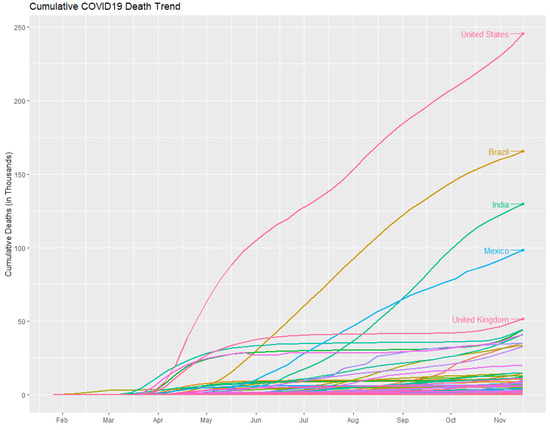
Figure A2.
Cumulative COVID-19 death numbers time trend.
Figure A2.
Cumulative COVID-19 death numbers time trend.
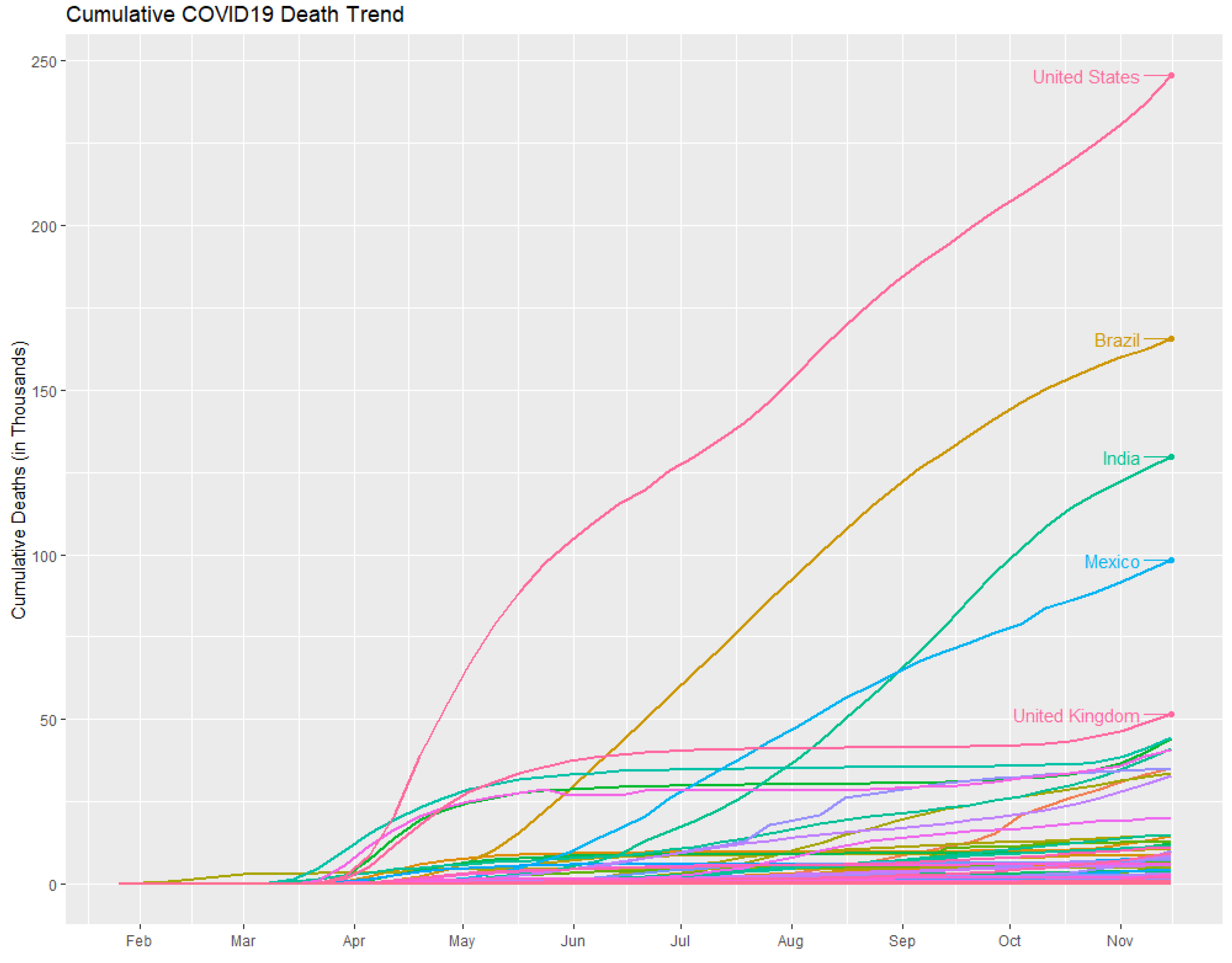
Table A1.
WDI variable description.
Table A1.
WDI variable description.
| Variable Name | WDI Variable Name | WDI Variable Definition |
|---|---|---|
| Employment.services.pct | Employment in service (percentage of total employment) (modeled ILO estimate) | Employment is defined as persons of working age who were engaged in any activity to produce goods or provide services for pay or profit, whether at work during the reference period or not at work due to temporary absence from a job, or to working-time arrangement. The services sector consists of wholesale and retail trade and restaurants and hotels; transport, storage, and communications; financing, insurance, real estate, and business services; and community, social, and personal services, in accordance with divisions 6–9 (ISIC 2) or categories G-Q (ISIC 3) or categories G-U (ISIC 4). |
| Employment.industry.pct | Employment in industry (percentage of total employment) (modeled ILO estimate) | Employment is defined as persons of working age who were engaged in any activity to produce goods or provide services for pay or profit, whether at work during the reference period or not at work due to temporary absence from a job, or to working-time arrangement. The industry sector consists of mining and quarrying, manufacturing, construction, and public utilities (electricity, gas, and water), in accordance with divisions 2–5 (ISIC 2) or categories C–F (ISIC 3) or categories B–F (ISIC 4). |
| Pop.in.urban.agg.more.than.1m.pct | Population in urban agglomerations of more than 1 million (percentage of total population) | Population in urban agglomerations of more than one million is the percentage of a country’s population living in metropolitan areas that in 2018 had a population of more than one million people. |
| GDP.per.capita | GDP per capita (constant 2010 US$) | GDP per capita is gross domestic product divided by midyear population. GDP is the sum of gross value added by all resident producers in the economy plus any product taxes and minus any subsidies not included in the value of the products. It is calculated without making deductions for depreciation of fabricated assets or for depletion and degradation of natural resources. Data are in constant 2010 USD. |
| Tourism.inflows | International tourism, number of arrivals | International inbound tourists (overnight visitors) are the number of tourists who travel to a country other than that in which they usually reside, and outside their usual environment, for a period not exceeding 12 months and whose main purpose in visiting is other than an activity remunerated from within the country visited. When data on the number of tourists are not available, the number of visitors, which includes tourists, same-day visitors, cruise passengers, and crew members, is shown instead. |
| safely managed sanitation services (percentage of population) | People using safely managed sanitation services (percentage of population) | The percentage of people using improved sanitation facilities that are not shared with other households and where excreta are safely disposed of in situ or transported and treated offsite. Improved sanitation facilities include flush/pour flush to piped sewer systems, septic tanks, or pit latrines: ventilated improved pit latrines, compositing toilets or pit latrines with slabs. |
| Trade.pct | Trade (percentage of GDP) | Trade is the sum of exports and imports of goods and services measured as a share of gross domestic product. |
| Savings.pct | Gross domestic savings percentage of GDP) | Gross domestic savings are calculated as GDP less final consumption expenditure (total consumption). |
| Trade.pct | Trade (percentage of GDP) | Trade is the sum of exports and imports of goods and services measured as a share of gross domestic product. |
References
- Van Doremalen, N.; Bushmaker, T.; Morris, D.H.; Holbrook, M.G.; Gamble, A.; Williamson, B.N.; Tamin, A.; Harcourt, J.L.; Thornburg, N.J.; Gerber, S.I.; et al. Aerosol and surface stability of SARS-CoV-2 as compared with SARS-CoV-1. N. Engl. J. Med. 2020, 382, 1564–1567. [Google Scholar] [CrossRef] [PubMed]
- Hammett, E. How long does Coronavirus survive on different surfaces? BDJ Team 2020, 7, 14–15. [Google Scholar] [CrossRef]
- Hale, T.; Angrist, N.; Goldszmidt, R.; Kira, B.; Petherick, A.; Phillips, T.; Webster, S.; Cameron-Blake, E.; Hallas, L.; Majumdar, S.; et al. A global panel database of pandemic policies (Oxford COVID-19 Government Response Tracker). Nat. Hum. Behav. 2021, 5, 529–538. [Google Scholar] [CrossRef] [PubMed]
- Ebrahim, S.H.; Memish, Z.A. COVID-19–the role of mass gatherings. Travel Med. Infect. Dis. 2020, 34, 101617. [Google Scholar] [CrossRef] [PubMed]
- Breitenfellner, A.; Hildebrandt, A. High employment with low productivity? The service sector as a determinant of economic development. Monet. Policy Economy 2006, 1, 110–135. [Google Scholar]
- Welsch, R.; Wessels, M.; Bernhard, C.; Thönes, S.; von Castell, C. Physical distancing and the perception of interpersonal distance in the COVID-19 crisis. Sci. Rep. 2021, 11, 11485. [Google Scholar] [CrossRef]
- Jordan, R.E.; Adab, P.; Cheng, K.K. COVID-19: Risk factors for severe disease and death. BMJ 2020, 368, m1198. [Google Scholar] [CrossRef] [PubMed] [Green Version]
- Zhou, F.; Yu, T.; Du, R.; Fan, G.; Liu, Y.; Liu, Z.; Xiang, J.; Wang, Y.; Song, B.; Gu, X.; et al. Clinical course and risk factors for mortality of adult inpatients with COVID-19 in Wuhan, China: A retrospective cohort study. Lancet 2020, 395, 1054–1062. [Google Scholar] [CrossRef]
- Ashraf, B.N. Socioeconomic conditions, government interventions and health outcomes during COVID-19. COVID Econ. Vetted Real-Time Papers 2020, 37, 141–162. [Google Scholar]
- Gerritse, M. Cities and COVID-19 infections: Population density, transmission speeds and sheltering responses. COVID Econ. Vetted Real-Time Papers 2020, 37, 1–26. [Google Scholar]
- Paul, A.; Englert, P.; Varga, M. Socio-economic disparities and COVID-19 in the USA. J. Phys. Complex. 2021, 2, 035017. [Google Scholar] [CrossRef]
- Ghosh, S. Lockdown, pandemics and quarantine: Assessing the Indian evidence. COVID Econ. 2020, 37, 73–99. [Google Scholar]
- Ren, X. Pandemic and lockdown: A territorial approach to COVID-19 in China, Italy and the United States. Eurasian Geogr. Econ. 2020, 61, 423–434. [Google Scholar] [CrossRef]
- Das, S. Prediction of COVID-19 disease progression in india: Under the effect of national lockdown. arXiv 2020, arXiv:2004.03147. [Google Scholar]
- Global Economic Prospects; World Bank: Washington, DC, USA, 2020.
- Demombynes, G. COVID-19 Age-Mortality Curves Are Flatter in Developing Countries; Policy Research Working Paper; no. WPS 9313; COVID-19 (Coronavirus); World Bank Group: Washington, DC, USA, 2020; Available online: http://documents.worldbank.org/curated/en/701441593610141326/COVID-19-Age-Mortality-Curves-Are-Flatter-in-Developing-Countries (accessed on 2 August 2020).
- Schellekens, P.; Sourrouille, D.M. COVID-19 Mortality in Rich and Poor Countries: A Tale of Two Pandemics? World Bank Policy Research Working Paper No. 9260; World Bank: Washington, DC, USA, 2020; Available online: https://ssrn.com/abstract=3614141 (accessed on 15 June 2020).

Publisher’s Note: MDPI stays neutral with regard to jurisdictional claims in published maps and institutional affiliations. |
© 2021 by the authors. Licensee MDPI, Basel, Switzerland. This article is an open access article distributed under the terms and conditions of the Creative Commons Attribution (CC BY) license (https://creativecommons.org/licenses/by/4.0/).