Article

Carbon Emissions and Brazilian Ethanol Prices: Are They Correlated? An Econophysics Study

by
Derick David Quintino
1,*,
Heloisa Lee Burnquist
1 and
Paulo Jorge Silveira Ferreira
2,3,4
1
Department of Economics, Administration and Sociology, Luiz de Queiroz—College of Agriculture, University of São Paulo, Piracicaba 13418-900, SP, Brazil
2
VALORIZA—Research Center for Endogenous Resource Valorization, 7300-555 Portalegre, Portugal
3
Instituto Politécnico de Portalegre, 7300-110 Portalegre, Portugal
4
CEFAGE-UE, IIFA, Universidade de Évora, Largo dos Colegiais 2, 7004-516 Évora, Portugal
*
Author to whom correspondence should be addressed.
Sustainability 2021, 13(22), 12862; https://doi.org/10.3390/su132212862
Submission received: 29 September 2021 / Revised: 8 November 2021 / Accepted: 16 November 2021 / Published: 20 November 2021
(This article belongs to the Special Issue The Economics of Greenhouse Gases Emission Reduction)

Abstract

:
Brazil is one of the largest global producers and exporters of ethanol and in 2017 launched RenovaBio, a programme aiming to mitigate greenhouse gas emissions. In parallel to this domestic scenario, there is rapid growth in the world market of carbon production, as well as complex price relations between fossil and renewable energies becoming increasingly important in recent years. The present work aims to contribute to filling a gap in knowledge about the relationship between Brazilian ethanol and other relevant energy-related commodities. We use a recent methodology (Detrended Cross-Correlation Approach—DCCA—with sliding windows) to analyze dynamically the cross-correlation levels between Brazilian ethanol prices and carbon emissions, as well as other possible-related prices, namely: sugar, Brent oil, and natural gas prices, with a sample of daily prices between January 2010 and July 2020. Our results indicate that (i) in the whole period, Brazilian ethanol has significant correlations with sugar, moderate correlation with oil in the short term, and only a weak, short-term correlation with carbon emission prices; (ii) with a sliding windows approach, the strength of the correlation between ethanol and carbon emissions varies between weak and non-significant in the short term.

1. Introduction

Due to policies stemming from global climate change, many governments encourage the use of biofuels through subsidies or mandate policies [1]. Developing countries, including Brazil, are likely to play an important role in the biofuels market in the coming years [2].
Brazil is an important global player in the ethanol market, and the use of renewable energies is a robust strategy in order to achieve sustainable development. In addition, Brazilian ethanol is fully competitive with gasoline as a substitute fuel, and its use is consolidated through the large fleet of flex-fuel vehicles in Brazil [3]. In addition to ethanol, sugarcane originates another important product for Brazilian and global agribusiness, namely, sugar. Brazil is responsible for at least 50% of all sugar exported on the international market, due to its economically competitive production and export capacity [4].
Santos and Ferreira Filho [5] argue that the substitution of fossil fuels by renewables, ethanol and biodiesel, has the potential to reduce the emission of pollutants without additional cost to the Brazilian GDP.
Goldemberg [6] highlights that Brazilian ethanol production is the most important and structured example of a large-scale renewable energy program in 2000s, and this was a decision supported by civil society and other agents involved in this process, such as the agricultural and industrial sugar-energy sector and the automobile industry. With the advent of flex-fuel cars, Brazil has consolidated its status as an economic reference in the search for sustainability [7]. Brazil was the leader in ethanol production until 2006, but since 2007 the US has taken the lead with Brazil in second position [3].
According to the Energy and Environment Institute [8], in the city of São Paulo (the most populous in the country, with more than 12 million inhabitants), automobiles are responsible for 72.6% of greenhouse gas emissions (GHG). Debone et al. [9] showed that, during the 90 days of social isolation in the city of São Paulo due to the COVID-19 health crisis, there was a significant improvement in air quality, avoiding hundreds of premature deaths and saving up to $ 1.5 billion in health care costs. Therefore, it is important that, considering both the economic point of view, and public and environmental health, there is greater substitution of fossil fuels by renewables. Renewable sources have contributed to lowering the amount of CO2 emissions into the atmosphere, as shown in Figure 1 [10], i.e., by using more ethanol than gasoline, the former acting as a substitute for the latter, there is mitigation of GHG emissions.
Another very important step in this direction was the creation of the National Biofuels Program, RenovaBio, in December 2017 [14]. RenovaBio creates a decarbonization market, through a financial bond called CBIO, which is issued by biofuel producers or importers. These securities are traded on the Brazilian Stock Exchange and are directly linked to the amount of reduction in the emission of greenhouse gases, GHG [15]. RenovaBio’s objective was not to create a carbon tax, offer subsidies, or create mandates for the use of biofuels instead of fossil fuels, but to establish a strategic role for biofuels of all types in the national energy matrix, both in terms of energy security and mitigation of GHG emissions [16]. It is important to point out that, through the composition of 27% of hydrated ethanol for the formulation of gasoline, this policy was responsible for a reduction of more than 300 million tons of CO2 in the period from March 2003 (beginning of production of flex-cars) to May 2015 [17]. For comparative purposes, this amount is equivalent to Poland’s annual emissions, considered one of the largest pollutants in the world due to the great use of coal [17].
According to Lee and Yoon [18], there are basically three reasons that bring the fossil energy markets closer to the renewable ones: (i) the use of fossil fuels increases carbon emissions; (ii) population and economic growth, especially in emerging countries, boost carbon emissions and their prices; (iii) the use of renewable energies can replace fossil energy and thus reduce carbon emissions. Through the integration of financial markets with energy products, both traditional (oil) and new markets (renewable energy and carbon), the prices of such assets may be more closely correlated.
Dutta [19] studied the relationship between carbon emission prices and biodiesel in the European Union and found that both prices move in the same direction. In addition, price correlations are dynamic, that is, they tend to vary over time. Finally, the author suggests that the price risks of clean energy stocks can be diversified if investors include both renewable energy assets and a commodity volatility index in their portfolio.
Since its inception, the European Union’s emissions trading system (EU-ETS) has been very efficient in reducing greenhouse gas (GHG) emissions, and in 2015, the volume of GHGs in the EU−28 was 22% below the 1990s levels, which means a decrease of 1265 million tonnes of CO2 equivalent [20]. In this way, the European Union Allowance (EUA) emerged as an important financial sector. It is noteworthy that the EU-ETS is the largest carbon emission allowance market, representing 84% of the global carbon market value. [20].
Dutta and Bouri [20] found that a rise in carbon emission prices tends to increase Brazilian ethanol prices, supporting the hypothesis that carbon emissions and ethanol prices move in the same direction. The authors claim that this result is not surprising, given that higher carbon prices encourage investments in ethanol, which can cause an increase in its price. They also found that the intensity of volatility jumps varies with time, and it is persistent, that is to say, a high probability of many (few) jumps today tends to be followed by many (few) jumps tomorrow.
It is important to note that the relationship between Brazilian ethanol prices and carbon emissions is little explored in the literature, and to the best of our knowledge, the only work is the innovative investigation by [20].
Our investigation aims to expand the investigation of [20] by verifying whether carbon emission prices are correlated with Brazilian hydrated ethanol prices, in different time scales, both in the short and long run. This issue is relevant because the questions about the impact of carbon emission prices upon a key biofuel source, such as bioethanol, tend to focus on its early stages.
There are a myriad of agents (government, industry, and financial institutions, among others) that are interested in whether these price linkages have different horizons such that different investment returns can be expected over time. Therefore, we intend to offer new evidence that could be important to the society as a whole and in particular to policymakers and investors.
The findings of Dutta and Bouri [20] would lead to the expectation that a rise in carbon emission prices is positively related to ethanol prices, such that these should move in the same direction. However, new questions arise when the long-run trends are important for decision making. Assuming that a great amount of investment is made on less-carbon emission fuel production, such as bioethanol, it could be expected that in the short run, a positive relationship between the price at both ethanol and CO2 emissions could prevail. However, as more bioethanol is produced, its price tends to decrease. Should one expect that carbon emission prices are also expected to decrease due to that? What if people start to value more those companies that invest in decreasing CO2 emissions not necessarily related to fuel production? Is there any reason to expect that CO2 related bonds would also decrease in the longer run? In this paper, we expect to bring new evidence to contribute to this debate.
Therefore, the main objective of this research is to investigate the cross-correlation between Brazilian ethanol prices and carbon emission prices. Besides analysis of the degree of association between ethanol and carbon emission prices, we also analyze the relationship with oil prices (as a dirty energy), natural gas (a quasi-dirty one), and sugar prices, due to Brazilian sugar and ethanol originating in sugarcane [3].
Using daily data, and including underexplored commodities in relation to biofuels, such as carbon emission prices, which have the appeal of being environmentally friendly, we also contribute to the growing literature on ESG investments. Secondly, we use a recent and robust methodology, a dynamic version of the DCCA, as we consider a sliding windows approach [21,22], which in addition to having the relevant properties of its static counterpart, can provide a dynamic view of the forces of association and thus the effects of shocks on market movements, as well as their changes and trends. Thirdly, as our sample has a daily periodicity, it provides a larger sample and a high frequency follow-up between these markets. The size of the sample is another important feature of this study, being in line with the study by Dutta and Bouri [20], which ends in 2017, allowing us to capture important effects such as the beginning of RenovaBio, launched in 2017, the 2018 lorry-driver crisis, and the emergence of COVID-19 on the global stage.
We develop a dynamic cross-correlation analysis (DCCA) as proposed by [21,22], using a sliding windows approach. The DCCA coefficient was proposed by [23] in order to analyze the correlation of two series efficiently [24], with desirable properties [25] and in various time scales, not restricted to the short-term versus long-term dichotomy.
This article is structured as follows: after this introduction, Section 2 contains the review of the literature, Section 3 presents the methods and data, Section 4 analyzes the results, and finally, Section 5 presents the conclusions.

2. Brief Literature Review

The literature contains several studies and debates about the relationship between the prices of ethanol and other assets, as is the case of the debate on food versus fuel prices, which can be followed through an excellent survey by [2]. In particular, Table 1 identifies the main investigations in this survey that involve Brazilian ethanol directly. For a more comprehensive view, involving not only ethanol but also biofuels in general in several countries or economic blocks, with emphasis on the US and European Union, see [2].
In economics and finance, there is substantial literature already developed that has applied the DCCA method with the purpose of calculating cross-correlations in a robust framework. Those studies dealing with finance and sustainability include, among many others, the climate’s influence on stock prices [32] and the analysis of agricultural futures prices [33]. In addition, Wang et al. [34] studied the cross-correlations between energy markets (oil and natural gas) and carbon emission markets, through the DCCA and multifractal DCCA. Another application concerns the correlation between oil prices and renewable energy stock prices [35]. Fan et al. [36] studied the relationship between carbon prices and coal prices, in seven main locations in China, via DCCA. Ferreira et al. [37] used the DCCA to verify the possibility of portfolio diversification via assets of renewable energy companies. Ferreira and Loures [38] is another recent example of applying the DCCA in the context of renewable energy. In this case, to verify the correlation between the S&P Global Clean Energy Index and the New York Stock Exchange (NYSE) and oil prices.
Among previous studies related to the ethanol market (or related goods) in Brazil via DCCA, Siqueira Jr [39] et al. analyzed the correlations and cross-correlations in the Brazilian market for commodities (including sugar) and shares on the Brazilian stock exchange. More recently, Nascimento Filho et al. [40] studied the cross-correlations in the gasoline retail market in the main Brazilian capitals and Murari et al. [41] performed a comparative analysis of the Brazilian gasoline and ethanol markets. Lima et al. [42] studied the cross-correlations and partial cross-correlations of ethanol, sugar, and oil in Brazil.

3. Material and Methods
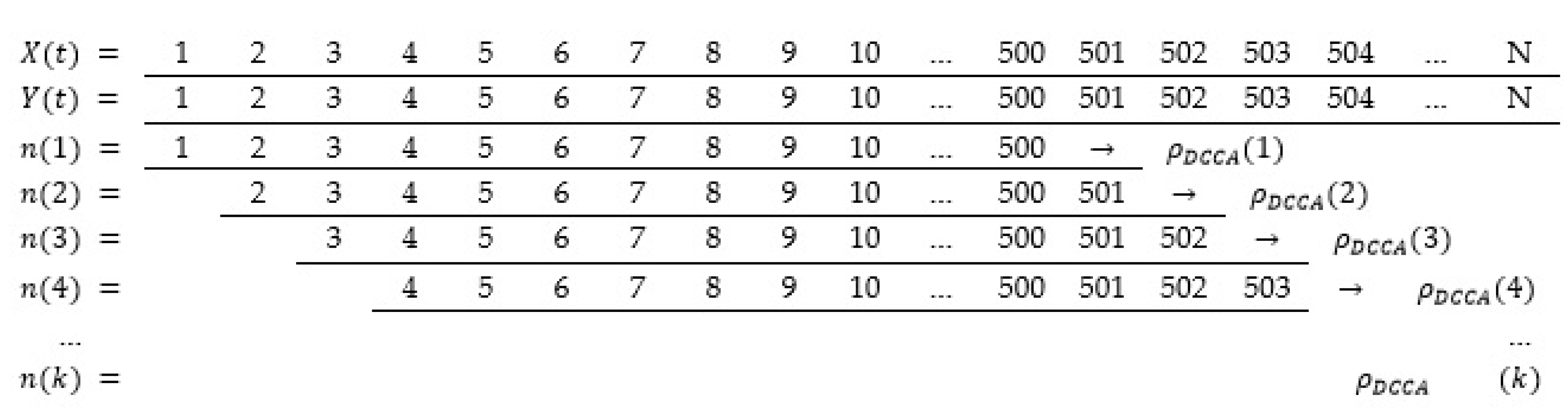
The present work uses daily data of future prices of carbon emissions (EU allowance) and Brazilian ethanol prices in the spot market. Oil prices (Brent type) are a reference for the Brazilian market [43,44], as well as for natural gas prices, which is also an important energy commodity [18,34]. Sugar prices refer to the New York contract number 11 (Sugar #11) due to its high liquidity and since it is a common price index used by agents operating in the Brazilian market (both domestic and international). Natural gas is the second largest energy commodity, but crude oil (WTI and Brent) is the main asset in this category, with more traded goods and financial contracts. According to Li [45], as of January 2016, natural gas accounts for 8.7% of the Dow Jones Commodity Index (DJCI), while crude oil accounts for 19.7%. Natural gas prices refer to the NYMEX Natural Gas Futures.
Therefore, these have been chosen as control variables (benchmark). We consider continuous future prices for the present analysis, since these assets are highly liquid for hedging or risk diversification for global economic agents. Carbon emissions, oil, natural gas, and sugar prices were collected through the Quandl platform (www.quandl.com, accessed on 23 August 2021). Regarding hydrated ethanol prices, we selected spot prices for the São Paulo market, calculated daily by CEPEA (Center for Advanced Studies on Applied Economics, https://www.cepea.esalq.usp.br/br, accessed on 23 August 2021). We chose to use the spot prices of Brazilian ethanol rather than the future prices of the Brazilian Stock Exchange (B3), since we considered it more representative of the market dynamics. As pointed out by [30,46,47], the futures contracts of the domestic stock exchange have low liquidity, with few contracts traded, being characterized as a thin market.
Energy commodities, more specifically oil and natural gas, have become an asset class used widely for diversification, hedging, or speculation. Investors, hedgers, speculators, and policy-makers have used these commodities as an alternative investment instrument, in order to protect themselves from equity market risk [48].
The analysis period is from 25 January 2010 to 31 July 2020, with a total of 2428 observations. The beginning of the sample is according to the emergence of the daily hydrated ethanol price indicator in Brazil. Figure 2 illustrates the behavior of price returns, r ( t ) , defined by r ( t ) = ln p t ln p t 1 , where p t is the asset price on date t.
Aiming to analyze the cross-correlations between Brazilian ethanol prices and carbon emissions prices, we use the dynamic DCCA with sliding windows, as recently proposed by [21,22] and also implemented as empirical strategy by [49,50]. Therefore, we present the DCCA proposed by [51] and DCCA correlation coefficient stated by [23]. In order to clarify the steps of the DCCA procedure, we split it into five steps, following the presentation of [40,41]
(i)
Consider two series x k and   y k where k = 1 , 2 ,     ,   N , with equidistant observations and calculate x ( t ) = k = 1 t x k and y ( t ) = k = 1 t y k .
(ii)
Next, we divide the sample in boxes of dimension n and so divided into ( N n ) overlapping boxes. The purpose of this procedure is to calculate local trends x ˜ ( t ) and y ˜ ( t ) of each series through ordinary least squares (OLS) and estimate the trend of each box, linear in our case, and the size of each box is in the interval between 4 n N / 4 .
(iii)
Subsequently, we calculate the difference between the original series and the estimated trend, in order to obtain a series without trend (detrended), and thus, we calculate the detrended covariance of the residues of each box of both series, which are given by f D C C A 2 = 1 n 1 k = 1 i + n ( x k x ˜ k ) ( y k y ˜ k ) .
(iv)
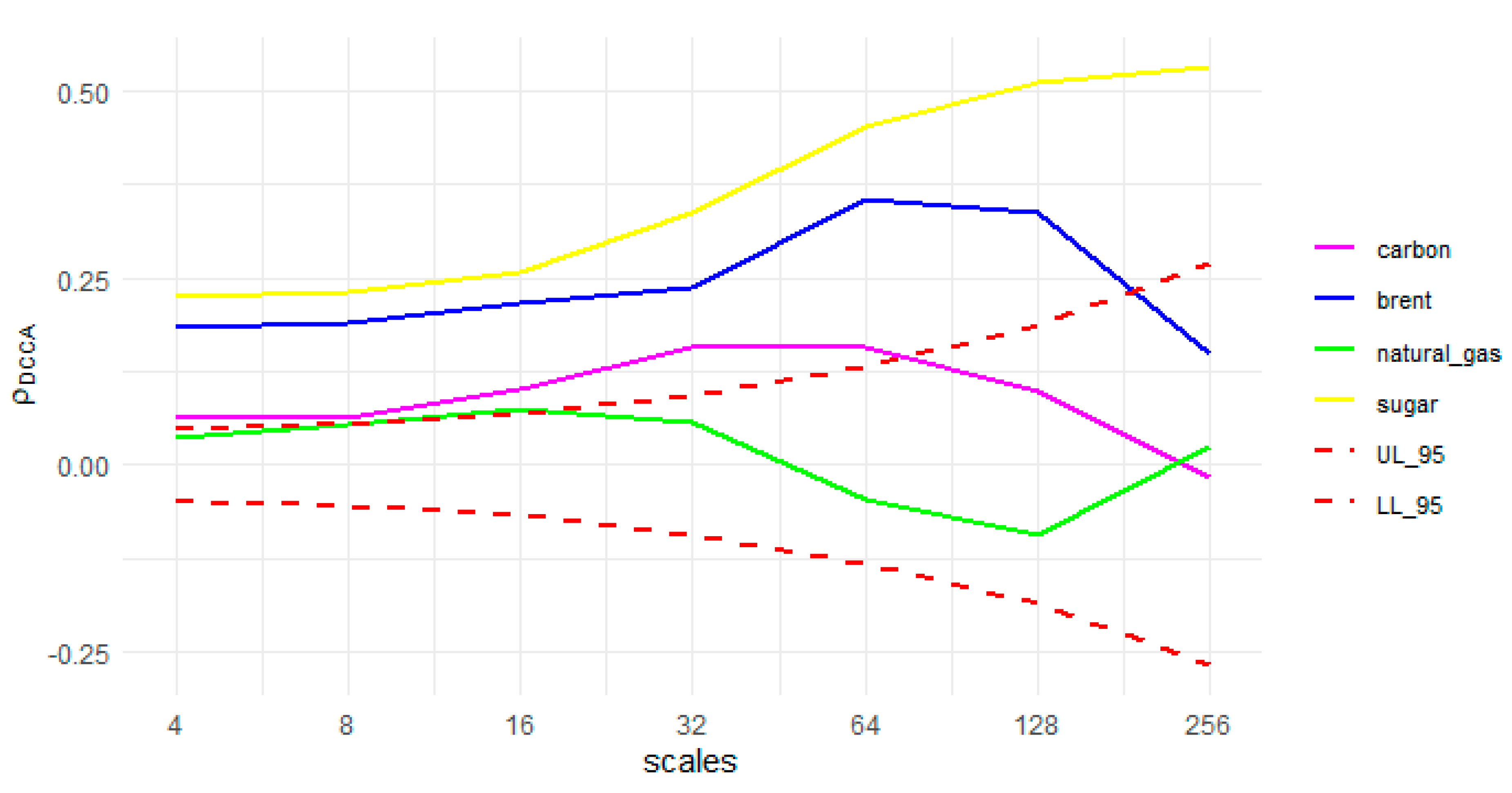
Afterwards, we have the sum of covariance of all boxes of size n, in order to obtain the detrended covariance given by F D C C A 2 ( n ) = 1 N n i = 1 N n f D C C A 2 . The process is continued for all lengths of the boxes, in order to obtain an expression for the relationship between DCCA fluctuations as a function of n. More specifically, the purpose is to find a relationship between F D C C A 2 ( n )   ~   n λ , where the parameter λ is the relevant one to evaluate the long-term cross-correlation. If λ > 0.5 , the series demonstrates a persistent long-term cross-correlation; in the case of λ < 0.5 , we have anti-persistent behavior, and finally if λ = 0.5 , there is no relationship between the variables.
(v)
Zebende [23] established the concept of the DCCA coefficient, ρ D C C A , based on the relationship between DFA (detrended fluctuation analysis) and DCCA, as ρ D C C A ( n ) = F D C C A 2 ( n ) F D F A { x } ( n )   F D F A { y } ( n ) , where D F A { x } and D F A { y } measure the degree of long-term dependence of each individual series, according to the definition of [52].
According to [24], the DCCA coefficient is efficient. Furthermore, it is between -1 as the minimum value (perfect anti-correlation) and +1 as the maximum value (perfect correlation), namely, 1 ρ D C C A 1, and in the case of a null value ( ρ D C C A = 0 ) , we have the absence of correlation [24]. In addition, the critical values of ρ D C C A as a function of time scales were calculated by [53], so that we can test its statistical validity.
Similar to [22], we use a moving sample with 500 observations, and due to the use of sliding windows, we can have scales between 4 and 128 days. In addition, considering that we have data on a daily basis, the 128-day interval (about 6 months) can be seen as a long-term analysis. A useful illustration of how the sliding window calculation is performed, given the sample size and as a function of time dynamics, is illustrated in Figure 3.

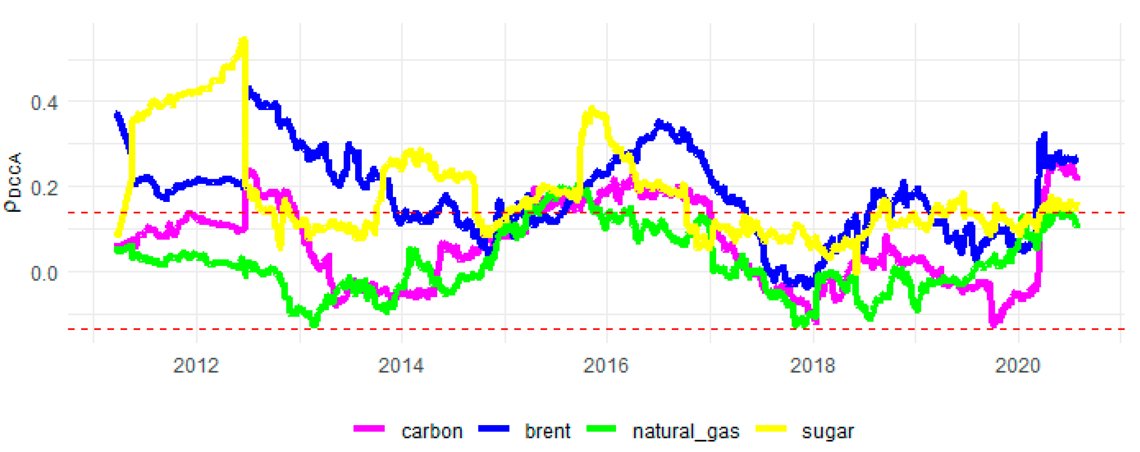
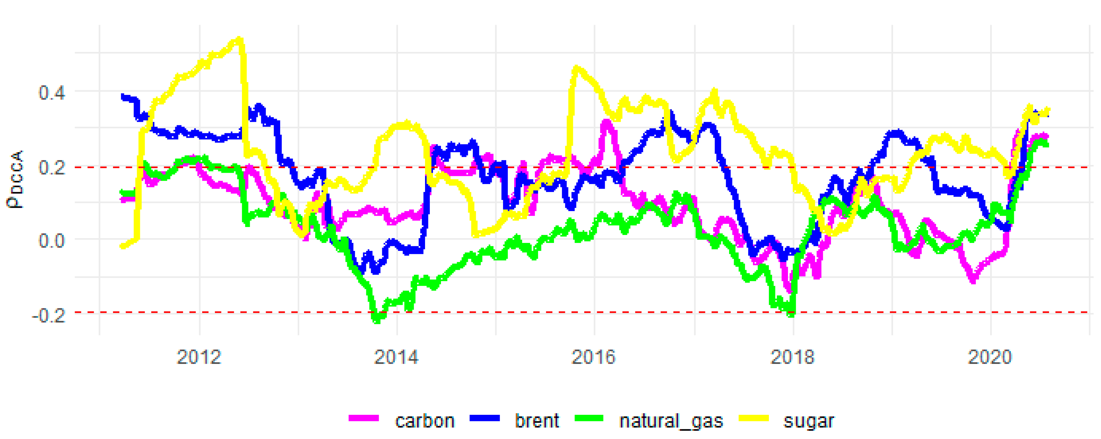
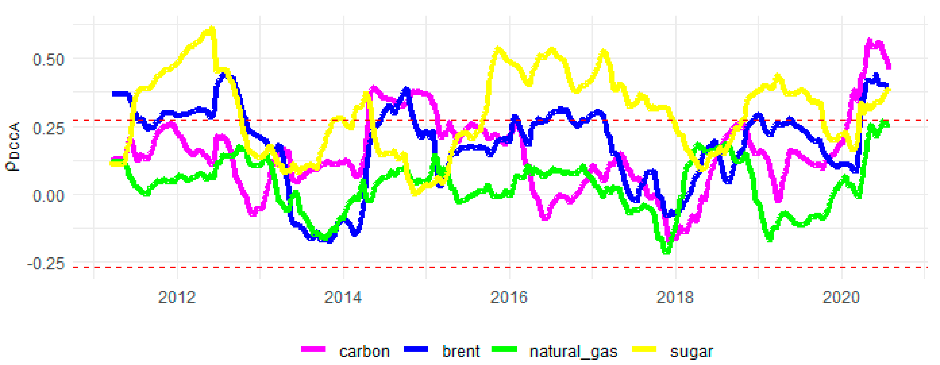
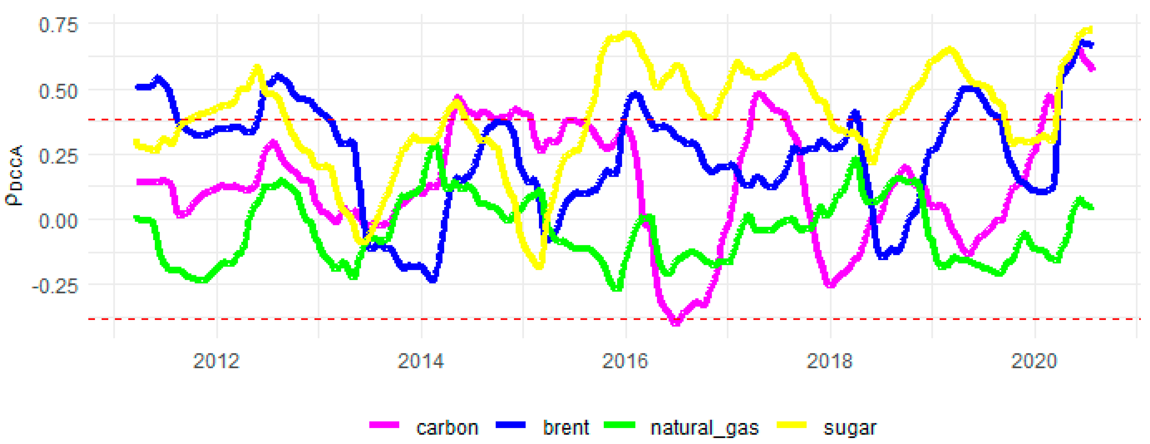
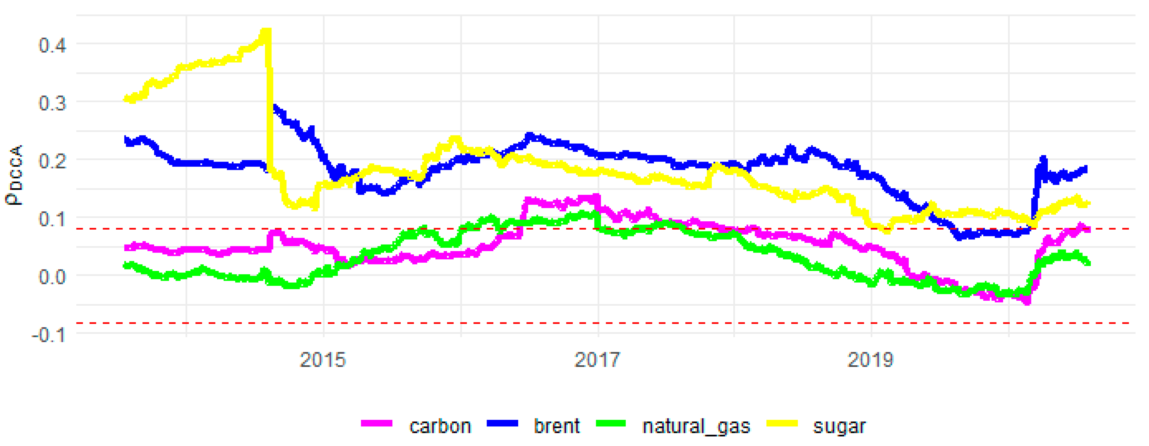
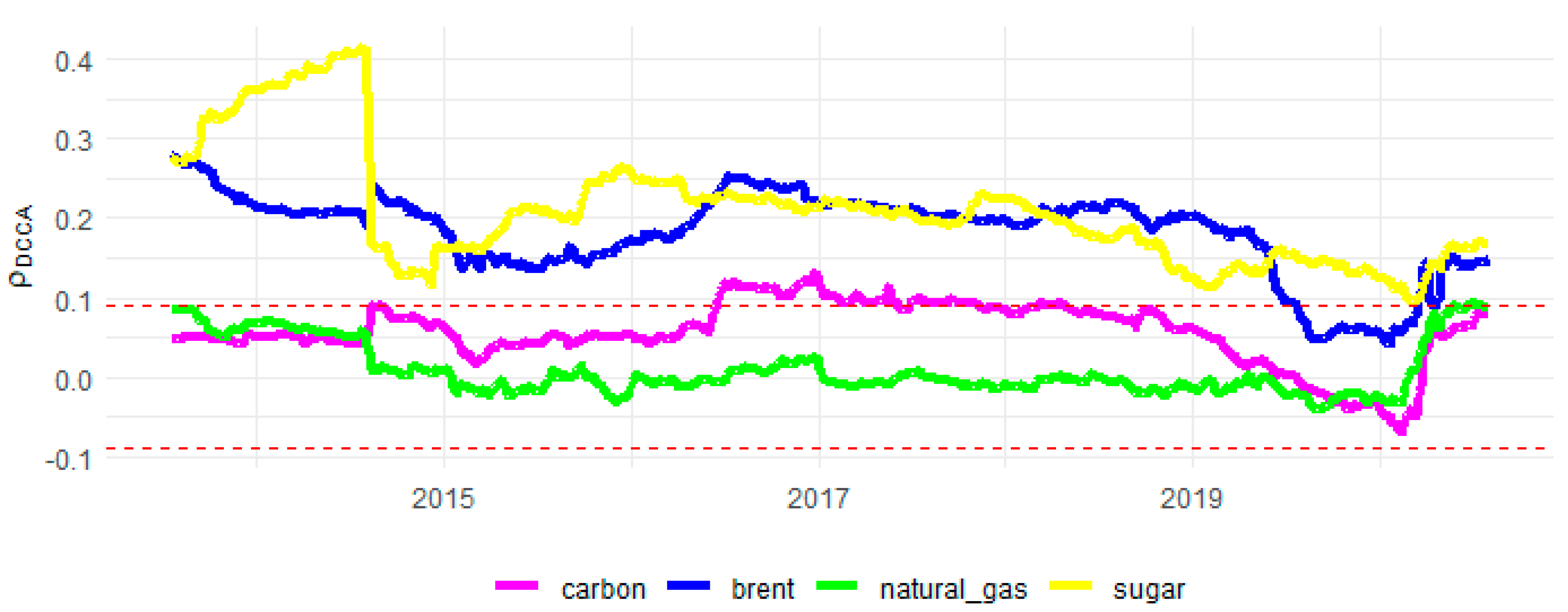
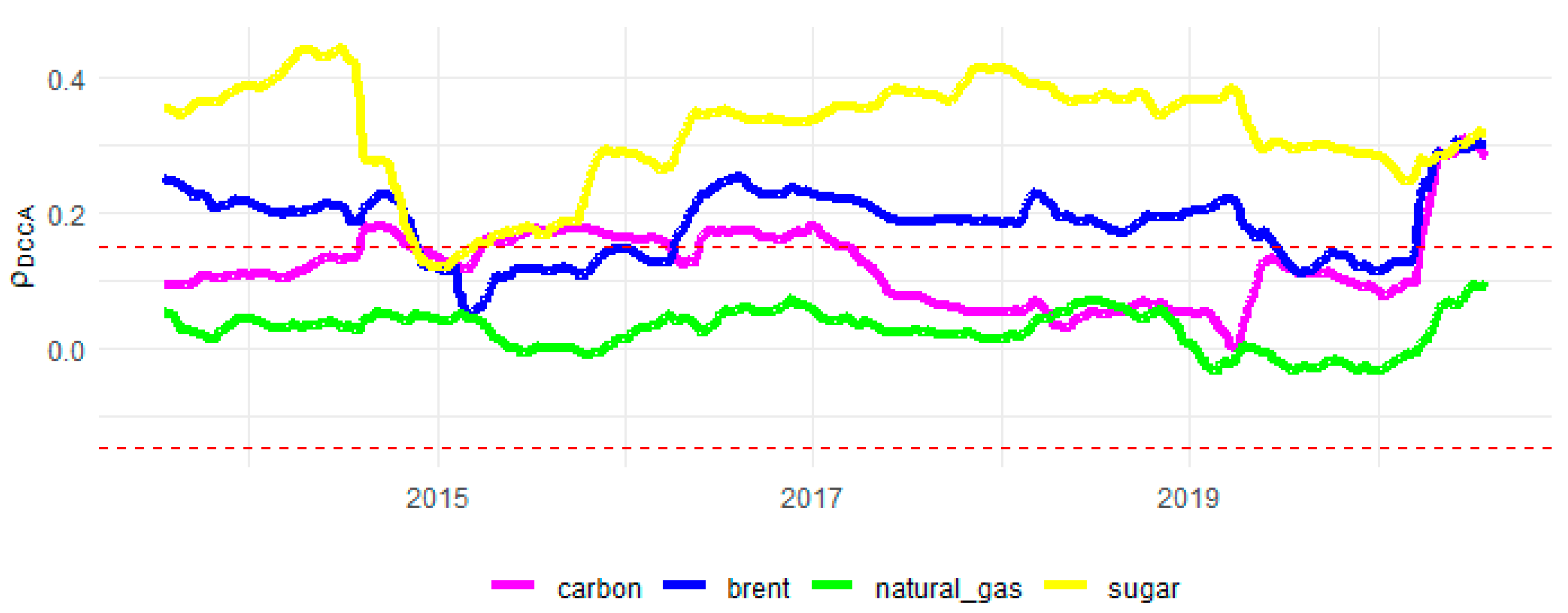
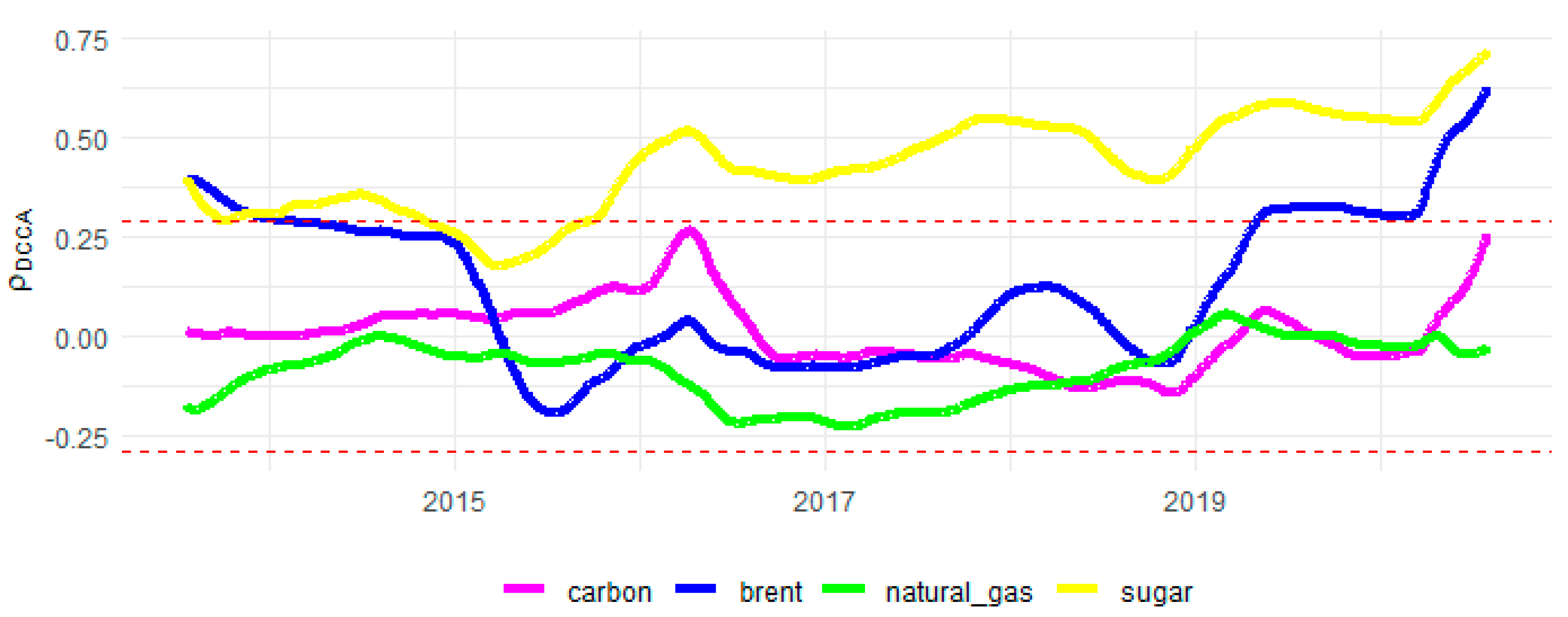
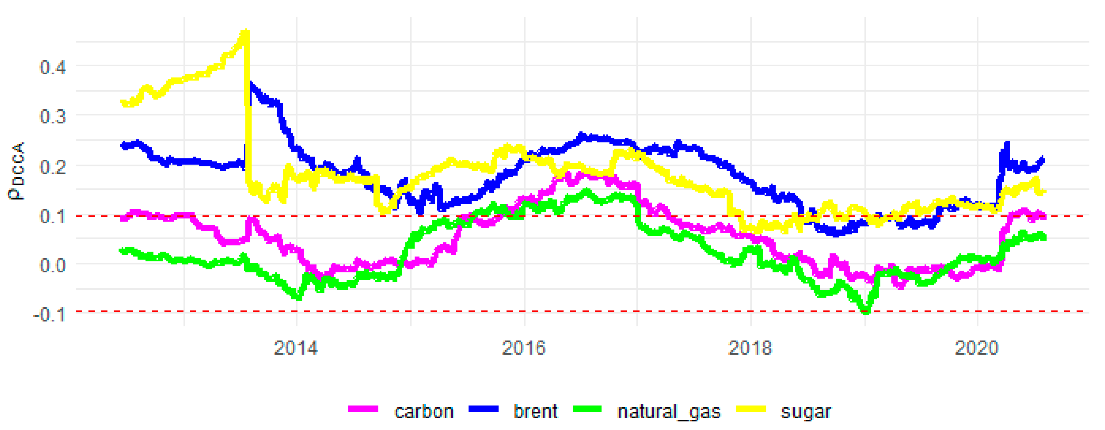
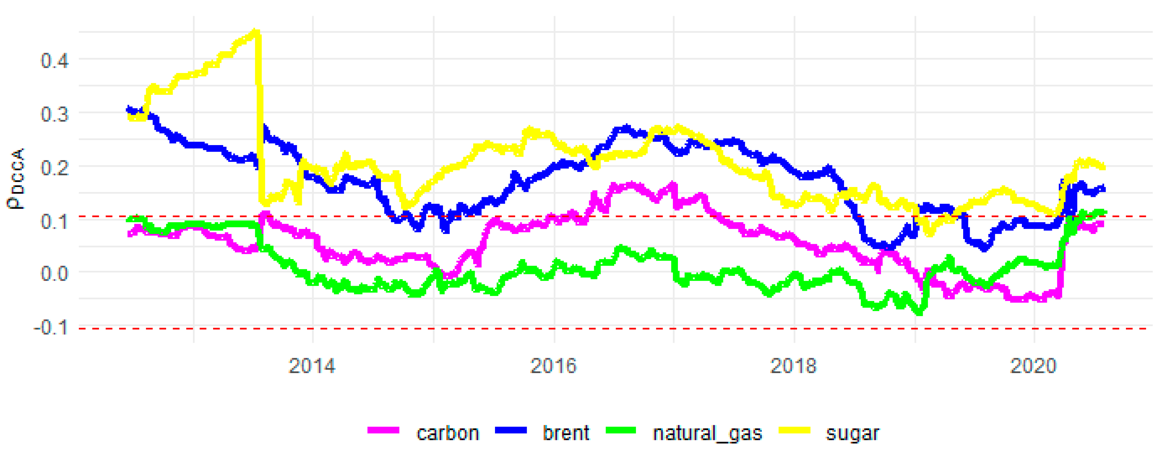
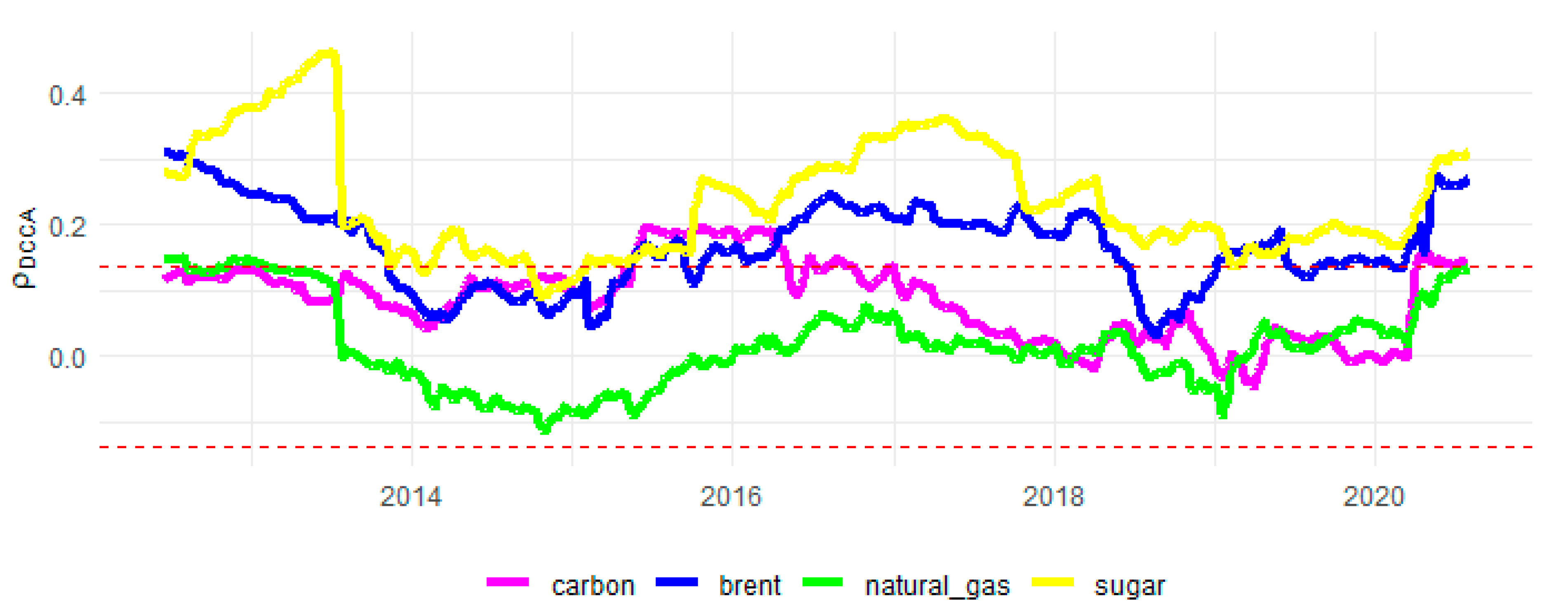
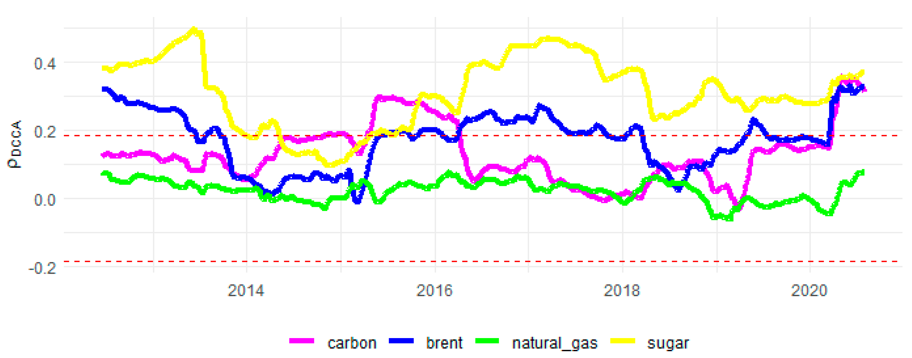
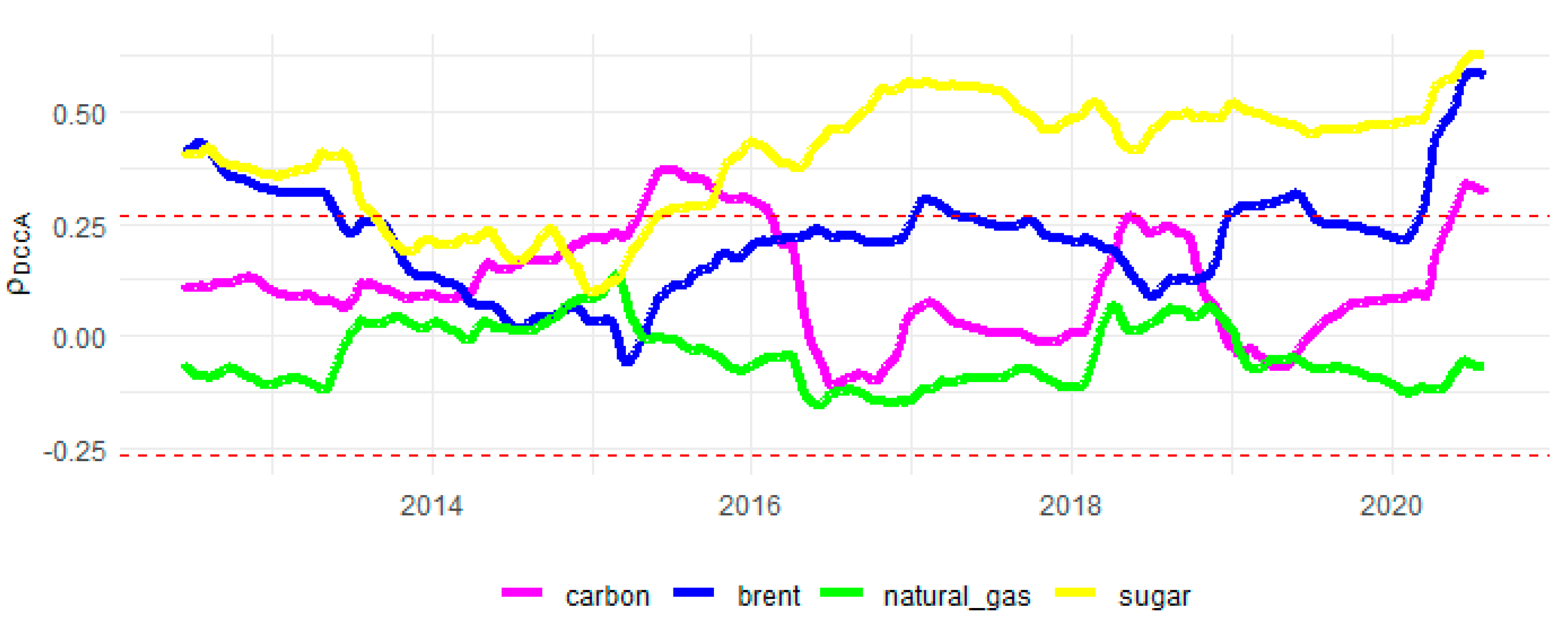
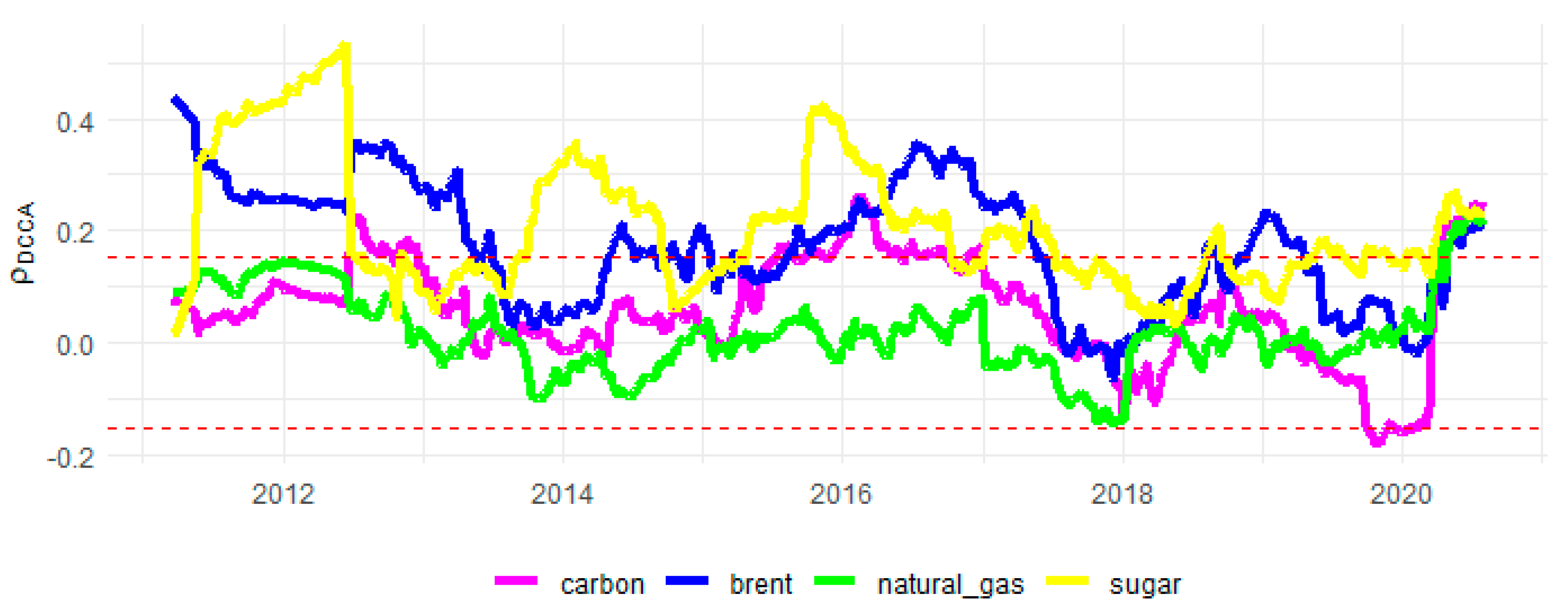
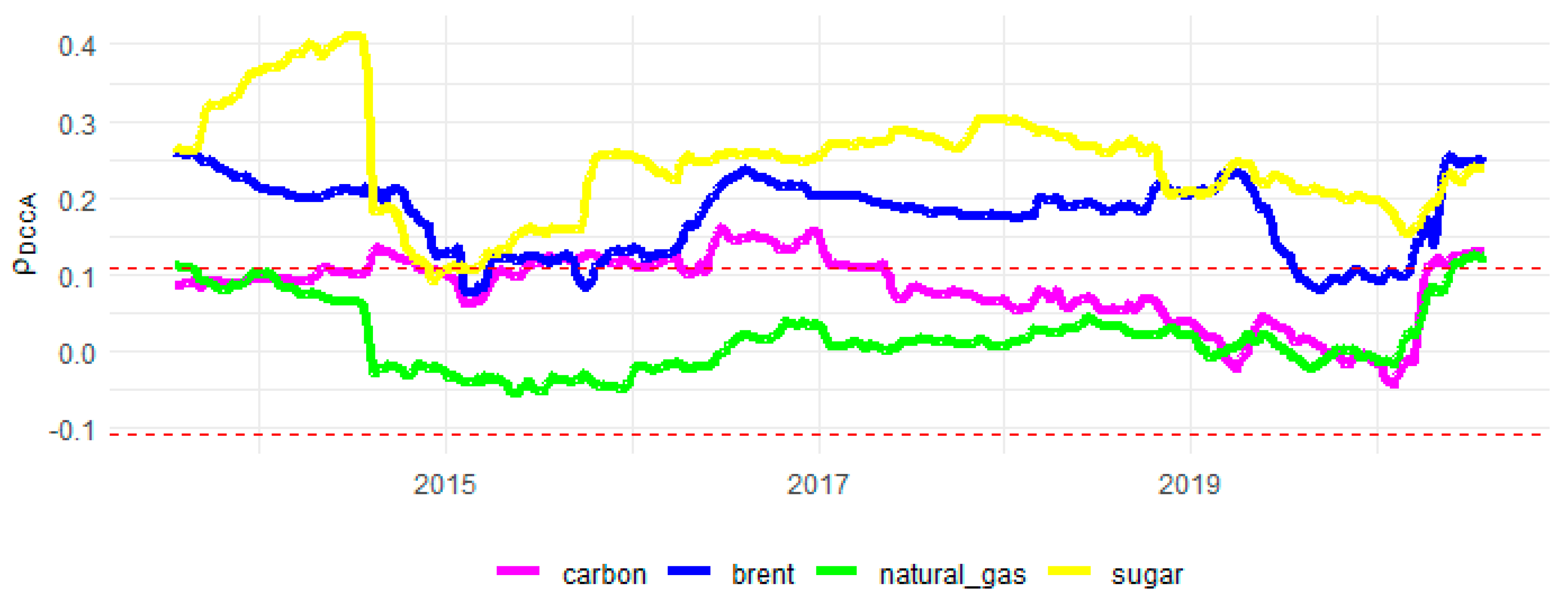
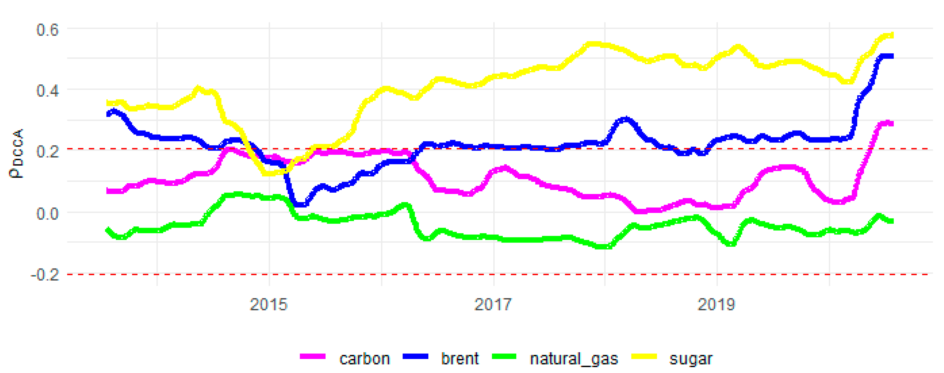
4. Results and Discussions

Figure 4 shows the results of the correlation coefficients between ethanol and the remaining commodities over time scales between 4 and 256 days (approximately 1 year). Values located between the lower and upper limits (dashed lines) are not statistically significant, whereas values above the upper limit and below the lower one has significance.
It can be seen that ethanol has a positive correlation with sugar during all the time scales, with an increased correlation in the long run (higher time scales). Regarding the other commodities, we can also see a significant and positive relationship with oil, during most of the time scales, although, in the long run, it is not significant. Regarding carbon, and despite the significance of the correlationship up to 64 days, correlation levels are lower, and, in the long run, they are not significant. Finally, considering natural gas, the evidence is of non-significance of the correlations.
In view of the recent changes in the dynamics of energy prices in the world, due to the coronavirus crisis and geopolitical aspects related to oil prices [18], as well as in the Brazilian ethanol market, with the new fuel pricing policy and the lorry-driver crisis [54], it is important to verify how the temporal dynamics of cross-correlations are dealt with.
In our next step, we will analyze the correlation dynamically, considering a fixed window (w) of 500 days, with time scales of 4, 8, 16, 32, 64, and 128 days. Figure 5, Figure 6, Figure 7, Figure 8, Figure 9 and Figure 10 have the values of the detrended cross-correlation analysis coefficient, ρ D C C A , as well as the confidence interval, namely, values of ρ D C C A that are between the dashed lines indicate that the correlation is not statistically significant. On the contrary, if the values of ρ D C C A are outside the dashed line limits (i.e., higher or lower values), they indicate that the correlations are statistically significant. Next, we will elucidate the results for each calculated time interval. For robustness purposes, we also employed the correlations using other window sizes, namely w = 250 (windows of about one year) and w = 750 (windows of about three years). The figures are presented in Appendix A (Figure A1, Figure A2, Figure A3, Figure A4, Figure A5, Figure A6, Figure A7, Figure A8, Figure A9, Figure A10 and Figure A11) and show qualitatively similar results.
In the four-day time interval (Figure 5), with the exception of a short time between 2016 and 2017, the correlation of ethanol with carbon emissions is not statistically significant, but is of weak magnitude, lower than 0.2. Similar behavior occurs with the correlation with natural gas. In relation to oil and sugar, the correlation is significant during most of the period under analysis, although with higher correlation levels until the end of 2013. In the case of oil, this result could be related to the sharp drop in its price, from approximately USD 100 per barrel in August 2014 to values close to USD 50 in January 2015 [55]. When considering both the 8-day window (Figure 6) and the 16-day window (Figure 7), the results are very similar, with no qualitative changes in the analysis made in the very short period of 4 days.
Changes in the pattern of correlations can be seen in the time scale of 32 days (Figure 8). We continue to observe a positive and almost always significant correlation with sugar price. Regarding carbon emissions, non-significant correlations are found, except in the period between 2015 and 2016, as well as more recently, in 2020, with the joint crisis of oil and coronavirus. In this case, in the post-COVID-19 period, the ethanol correlation gains strength and shows practically the same correlation pattern with oil. Regarding oil, correlation levels are significant at the beginning of the sample, as well as during some months between 2016 and 2017, and at the end of the sample post-2020, which could be related to the impact of the COVID-19 pandemic.
In the longer scales, namely 64 days (Figure 9) and 128 days (Figure 10), corresponding to the long run, we can see that ethanol just shows some significant correlation with sugar, especially post-2016, and more marginally with oil prices pre-2014, again showing strong force only during the COVID-19 pandemic period (post-2020). In this sense, we have evidence of the segmentation between the different assets, namely, sugar and oil versus carbon emissions and natural gas.
In addition, as stated by [56], the time varying correlation between crude oil and gas is not constant over time, because the two prices follow a completely divergent path, and this is why the correlation between them is reduced. The authors suggest that the shale revolution might have affected this volatility spillover. Therefore, in our investigation, this helps to explain why we have different correlation estimates between ethanol and oil and between ethanol and natural gas.
In order to develop the Brazilian ethanol market, aiming to be a global agent contributing to the fight against global warming, it is necessary to invest on three important fronts, among others: (i) productivity increases in the ethanol supply, (ii) greater energy efficiency of bi-fuel cars (flex), and (iii) ethanol price risk management mechanisms.
Firstly, Brazilian ethanol production has grown at an average rate of 1.2% per year in the last decade, much lower than the explosive growth of the 1970s, when ProÁlcool was created, and in the 2000s, with the emergence of flex fuel cars [16]. Almost all ethanol produced in Brazil is first generation ethanol, and therefore, it is necessary to invest in technological development for second generation (2G) ethanol [16,57]. This is already produced in Brazil, but the conversion process is still not established, and it is expected to be economically attractive by 2025 [16,57].
Regarding the second item, in 2012, through Decree 70819/12, the government’s Inovar-Auto program was launched, aiming to boost the level of innovation in the Brazilian automobile industry through incentives for investment in R&D, in order to produce safer and efficient use of energy, as only a small fraction of vehicles have energy-efficient technologies [58]. However, there was no evidence of the expected effect. On the contrary, it turned out to be a protectionist measure, giving tax exemption to domestic producers, in the face of international competition [58]. Furthermore, despite the high profit margin of the Brazilian automobile industry compared to those of the US and the European Union, large companies employ low-cost technologies for the domestic supply [58].
Finally, sugarcane, a raw material used in the production of both sugar and ethanol, has production cycles, with a harvest every 12 or 18 months, which is reflected in the seasonality of its final prices [41]. The first quarter of the year is the off-season period, where ethanol prices tend to be higher if there is not enough in stocks at mills and/or distributors [3]. The hydrated market is more dynamic than the anhydrous one (mixed with gasoline) and more subject to seasonality and competitive conditions in regional markets [47]. According to [59], a liquid ethanol futures market could reduce the different sources of uncertainty that affect biofuel prices, in order to provide more predictable bases for future prices and thus help manage the risk of these industries more efficiently. However, in the Brazilian case, as highlighted above, ethanol futures contracts did not show sufficient strength to create liquidity and thus does not offer a consolidated ethanol price risk management tool in the domestic market [30,46,47].
In this paper, we aim to contribute to understanding more clearly the possible connections of ethanol prices and therefore contribute to filling the gap regarding the third item.

5. Conclusions

In this article, using a robust dynamic cross-correlation methodology recently proposed by [21,22] and empirical evidence based on fresh data from the Brazilian ethanol spot prices and carbon emissions futures prices, we calculate the correlation between January 2010, the start of the Brazilian ethanol daily indicator, and July 2020. As a comparative framework for energy prices, the correlations of the Brazilian ethanol with the prices of Brent oil, natural gas, and sugar were also calculated. The price relations of carbon emissions and ethanol prices have not yet been sufficiently explored, and in this investigation, we seek to contribute to filling this gap. To the best of our knowledge, the notable exception is the investigation of [20].
The cross-correlations were considered in two scenarios: the first with a complete sample, and the second through sliding windows of 500 observations (approximately 2 years considering daily time series), in different time scales: 4, 8, 16, 32, 64, and 128 days. As a robustness test, we also consider other windows sizes (250 and 750 observations), which bring in general similar qualitative results of our basis scenario of 500 observations.
In the analysis of the complete sample, we observed that ethanol has a weak correlation with carbon emission prices, and only in the short term, that is, considering the scale of up to 64 days. In relation to sugar, as expected, we obtained an expressive and increasing positive association with larger scales. In comparison with oil prices, there is a statistically significant correlation, only in the short term, in our case, the period of less than 128 days, about 6 months. Finally, with natural gas, we do not observe any significant association.
Our results with regard to correlation between Brazilian ethanol with carbon emissions prices are somewhat different from those obtained by [20], which showed the existence of a positive correlation. Here, we have evidence of a weak or even non-significant correlation, mainly in the short run. Furthermore, the moving windows show that the correlation is time-dependent, varying according to the period analyzed, because in certain periods and specific time scales, no significant correlation is observed. However, it is important to note that the use of different methodologies and databases could be also relevant in explaining the different results.
In this sense, we believe that our results make an important contribution to decision-making by private sector agents in forming their portfolio and seeking assets with the potential to diversify market risks or hedging strategies, depending on the time horizon of analysis and the degree of protection they want to achieve. In addition to the long-term view, represented here by just over 10 years of series coexistence, moving windows provide a view of the short-term dynamics of the correlations between such assets. The results are also important for policy-makers, giving important information on the price dynamics of carbon emissions and Brazilian ethanol, as these prices reflect the trade-off of non-renewable energy versus an important source of clean energy.
It is important to note that our results also have implications for researchers. We found evidence that ethanol’s relationships with both oil and sugar are non-linear, and thus, the use of time series techniques that take this into account are appropriate in order to have a more robust view of the possible existence of such relationships. Furthermore, with the use of sliding windows, we have evidence of time-dependent behavior, with greater or lesser levels of correlation depending on current situations, such as the lorry drivers’ strike (May 2018) that paralyzed the Brazilian economy for weeks, as well as structural supply and demand shocks, in the wake of the outbreak and worsening of the COVID-19 crisis. Such shocks, especially if accompanied by changes in international oil prices, can cause great oscillation in the normal conditions of renewable energy prices, including Brazilian ethanol.
We also consider it could be interesting to use other different methodologies to assess the possible correlation changes in different market conditions, such as the cross-quantilogram methodology (see, for example, [60]), this being a possibility for future research.

Author Contributions

Conceptualization, D.D.Q., P.J.S.F. and H.L.B.; data curation, D.D.Q., P.J.S.F. and H.L.B.; formal analysis, D.D.Q., P.J.S.F. and H.L.B.; methodology, D.D.Q., P.J.S.F. and H.L.B.; writing—original draft, D.D.Q., P.J.S.F. and H.L.B.; writing—review and editing, D.D.Q., P.J.S.F. and H.L.B. All authors have read and agreed to the published version of the manuscript.

Funding

Derick Quintino and H.L.B. wish to acknowledge the CAPES for funding support. This study was financed in part by the Coordenação de Aperfeiçoamento de Pessoal de Nível Superior–Brasil (CAPES)–Finance Code 001. Paulo Ferreira also acknowledges the financial support of Fundação para a Ciência e a Tecnologia (grants UIDB/05064/2020 and UIDB/04007/2020).

Institutional Review Board Statement

Not applicable.

Informed Consent Statement

Not applicable.

Data Availability Statement

Data will be made available on request.

Acknowledgments

The authors are indebted to Marta Marjotta-Maistro, Jeronimo Santos and Luciano Rodrigues for helpful comments of an earlier version of this article. Usual disclaimers apply.

Conflicts of Interest

The authors declare no conflict of interest.

Appendix A

Figure A1. Evolution of the ρ D C C A between ethanol and the remaining commodities with time scales of 4 days and window size w = 250. Dashed lines represent critical values for statistical significance, according to [53].
Sustainability 13 12862 g0a1
Figure A2. Evolution of the ρ D C C A between ethanol and the remaining commodities with time scales of 8 days and window size w = 250. Dashed lines represent critical values for statistical significance, according to [53].
Sustainability 13 12862 g0a2
Figure A3. Evolution of the ρ D C C A between ethanol and the remaining commodities with time scales of 16 days and window size w = 250. Dashed lines represent critical values for statistical significance, according to [53].
Sustainability 13 12862 g0a3
Figure A4. Evolution of the ρ D C C A between ethanol and the remaining commodities with time scales of 32 days and window size w = 250. Dashed lines represent critical values for statistical significance, according to according to [53].
Sustainability 13 12862 g0a4
Figure A5. Evolution of the ρ D C C A between ethanol and the remaining commodities with time scales of 64 days and window size w = 250. Dashed lines represent critical values for statistical significance, according to according to [53].
Sustainability 13 12862 g0a5
Figure A6. Evolution of the ρ D C C A between ethanol and the remaining commodities with time scales of 4 days and window size w = 750. Dashed lines represent critical values for statistical significance, from the author’s calculations via GMZTests R package [61].
Sustainability 13 12862 g0a6
Figure A7. Evolution of the ρ D C C A between ethanol and the remaining commodities with time scales of 8 days and window size w = 750. Dashed lines represent critical values for statistical significance, from the author’s calculations via GMZTests R package [61].
Sustainability 13 12862 g0a7
Figure A8. Evolution of the ρ D C C A between ethanol and the remaining commodities with time scales of 16 days and window size w = 750. Dashed lines represent critical values for statistical significance, from author’s calculations via GMZTests R package [61].
Sustainability 13 12862 g0a8
Figure A9. Evolution of the ρ D C C A between ethanol and the remaining commodities with time scales of 32 days and window size w = 750. Dashed lines represent critical values for statistical significance, from the author’s calculations via GMZTests R package [61].
Sustainability 13 12862 g0a9
Figure A10. Evolution of the ρ D C C A between ethanol and the remaining commodities with time scales of 64 days and window size w = 750. Dashed lines represent critical values for statistical significance, from the author’s calculations via GMZTests R package [61].
Sustainability 13 12862 g0a10
Figure A11. Evolution of the ρ D C C A between ethanol and the remaining commodities with time scales of 128 days and window size w = 750. Dashed lines represent critical values for statistical significance, from the author’s calculations via GMZTests R package [61].
Sustainability 13 12862 g0a11

References

  1. Figueira, S.R.F.; Burnquist, H.L.; Bacchi, M.R.P. Forecasting fuel ethanol consumption in Brazil by time series models: 2006–2012. Appl. Econ. 2010, 42, 865–874. [Google Scholar] [CrossRef]
  2. Janda, K.; Kristoufek, L. The Relationship between Fuel and Food Prices: Methods and Outcomes. Annu. Rev. Resour. Econ. 2019, 11, 195–216. [Google Scholar] [CrossRef]
  3. David, S.A.; Quintino, D.D.; Inacio, C.M.C., Jr.; Machado, J.T. Fractional dynamic behavior in ethanol prices series. J. Comput. Appl. Math. 2018, 339, 85–93. [Google Scholar] [CrossRef]
  4. Costa, C.C.; Burnquist, H.L.; Guilhoto, J.J.M. Special safeguard tariff impacts on the Brazilian sugar exports. J. Int. Trade Law Policy 2015, 14, 70–85. [Google Scholar] [CrossRef]
  5. Santos, J.A.D.; Ferreira Filho, J.B.D.S. Substituição de Combustíveis Fósseis por Etanol e Biodiesel no Brasil e Seus Impactos Econômicos: Uma avaliação do Plano Nacional de Energia 2030. 2017. Available online: http://repositorio.ipea.gov.br/handle/11058/8231 (accessed on 15 July 2020).
  6. Goldemberg, J. Ethanol for a Sustainable Energy Future. Science 2007, 315, 808–810. [Google Scholar] [CrossRef] [Green Version]
  7. Coelho, S.T.; Goldemberg, J.; Lucon, O.; Guardabassi, P. Brazilian sugarcane ethanol: Lessons learned. Energy Sustain. Dev. 2006, 10, 26–39. [Google Scholar] [CrossRef]
  8. IEMA. Inventário De Emissões Atmosféricas Do Transporte Rodoviário De Passageiros No Município De São Paulo; IEMA: Sao Paulo, Brasil, 2020; Available online: http://emissoes.energiaeambiente.org.br/graficos (accessed on 10 September 2020).
  9. Debone, D.; Da Costa, M.; Miraglia, S. 90 Days of COVID-19 Social Distancing and Its Impacts on Air Quality and Health in Sao Paulo, Brazil. Sustainability 2020, 12, 7440. [Google Scholar] [CrossRef]
  10. EPE. Empresa de Pesquisa Energética. Análise de Conjuntura dos Biocombustíveis. 2019. Available online: http://www.mme.gov.br (accessed on 15 July 2020).
  11. EPE. Balanço Energético Nacional 2020: Ano-Base 2019; Empresa de Pesquisa Energética: Rio de Janeiro, Brazil, 2020. Available online: www.epe.gov.br (accessed on 15 July 2020).
  12. Rosa, L.P.; Oliveira, L.B.; Costa, A.O.; Pimenteira, C.A.; Mattos, L.B. Geração de Energia a partir de resíduos sólidos. In Tolmasquim, M.T (Coord) Fontes Alternativas, 515; Editora Interciência, COPPE, UFRJ: Rio de Janeiro, Brazil, 2003. [Google Scholar]
  13. MCTI. Fatores de Emissão de CO2 Para Utilizações que Necessitam do Fator Médio de Emissão do Sistema Interligado Nacional do Brasil, Como, por Exemplo, Inventários Corporativos; Ministério da Ciência, Tecnologia e Inovação: Brasília, Brazil, 2020. Available online: www.mct.gov.br (accessed on 15 July 2020).
  14. BRASIL. Lei n° 13.576, de 26 de Dezembro de 2017. Dispõe sobre a Política Nacional deBiocombustíveis (RenovaBio) e dá Outras Providências; Diário Oficial da União: Brasília, Brazil, 2017. Available online: www.planalto.gov.br (accessed on 15 July 2020).
  15. Klein, B.C.; Chagas, M.F.; Watanabe, M.D.B.; Bonomi, A.; Maciel Filho, R. Low carbon biofuels and the New Brazilian National Biofuel Policy (RenovaBio): A case study for sugarcane mills and integrated sugarcane-microalgae biorefineries. Renew. Sustain. Energy Rev. 2019, 115, 109365. [Google Scholar] [CrossRef]
  16. Karp, S.G.; Medina, J.D.C.; Letti, L.A.J.; Woiciechowski, A.L.; de Carvalho, J.C.; Schmitt, C.C.; Penha, R.D.O.; Kumlehn, G.S.; Soccol, C.R. Bioeconomy and biofuels: The case of sugarcane ethanol in Brazil. Biofuels Bioprod. Biorefining 2021, 15, 899–912. [Google Scholar] [CrossRef]
  17. da Rocha Lima Filho, R.I.; de Aquino, T.C.N.; Neto, A.M.N. Fuel price control in Brazil: Environmental impacts. Environ. Dev. Sustain. 2021, 23, 9811–9826. [Google Scholar] [CrossRef]
  18. Lee, Y.; Yoon, S.-M. Dynamic Spillover and Hedging among Carbon, Biofuel and Oil. Energies 2020, 13, 4382. [Google Scholar] [CrossRef]
  19. Dutta, A. Impact of carbon emission trading on the European Union biodiesel feedstock market. Biomass-Bioenergy 2019, 128, 105328. [Google Scholar] [CrossRef]
  20. Dutta, A.; Bouri, E. Carbon emission and ethanol markets: Evidence from Brazil. Biofuels Bioprod. Biorefining 2019, 13, 458–463. [Google Scholar] [CrossRef]
  21. Guedes, E.F.; Zebende, G.F. DCCA cross-correlation coefficient with sliding windows approach. Phys. A Stat. Mech. Appl. 2019, 527, 121286. [Google Scholar] [CrossRef]
  22. Tilfani, O.; Ferreira, P.; Boukfaoui, E.; Youssef, M. Dynamic cross-correlation and dynamic contagion of stock markets: A sliding windows approach with the DCCA correlation coefficient. Empir. Econ. 2021, 60, 1127–1156. [Google Scholar] [CrossRef]
  23. Zebende, G. DCCA cross-correlation coefficient: Quantifying level of cross-correlation. Phys. A Stat. Mech. Appl. 2011, 390, 614–618. [Google Scholar] [CrossRef]
  24. Kristoufek, L. Measuring correlations between non-stationary series with DCCA coefficient. Phys. A Stat. Mech. Appl. 2014, 402, 291–298. [Google Scholar] [CrossRef] [Green Version]
  25. Zhao, X.; Shang, P.; Huang, J. Several fundamental properties of dcca cross-correlation coefficient. Fractals 2017, 25, 1750017. [Google Scholar] [CrossRef]
  26. Rapsomanikis, G.; Hallam, D. Threshold Cointegration in the Sugar-Ethanol-Oil Price System in Brazil: Evidence from Nonlinear Vector Error Correction Models; FAO Commodity and Trade Policy Research Working Paper, 22; FAO: Rome, Italy, 2006. [Google Scholar]
  27. Serra, T.; Zilberman, D.; Gil, J. Price volatility in ethanol markets. Eur. Rev. Agric. Econ. 2011, 38, 259–280. [Google Scholar] [CrossRef] [Green Version]
  28. Kristoufek, L.; Janda, K.; Zilberman, D. Comovements of ethanol-related prices: Evidence from Brazil and the USA. GCb Bioenergy 2016, 8, 346–356. [Google Scholar] [CrossRef] [Green Version]
  29. Bentivoglio, D.; Finco, A.; Bacchi, M.R.P. Interdependencies between biofuel, fuel and food prices: The case of the Brazilian ethanol market. Energies 2016, 9, 464. [Google Scholar]
  30. Capitani, D.H.D.; Junior, J.C.C.; Tonin, J.M. Integration and hedging efficiency between Brazilian and US ethanol markets. Contextus 2018, 16, 93–117. [Google Scholar] [CrossRef]
  31. Dutta, A. Cointegration and nonlinear causality among ethanol-related prices: Evidence from Brazil. GCB Bioenergy 2018, 10, 335–342. [Google Scholar] [CrossRef] [Green Version]
  32. Cao, G.; Han, Y. Does the weather affect the Chinese stock markets? Evidence from the analysis of DCCA cross-correlation coefficient. Int. J. Mod. Phys. B 2014, 29, 1450236. [Google Scholar] [CrossRef]
  33. Cao, G.; He, C.; Xu, W. Effect of Weather on Agricultural Futures Markets on the Basis of DCCA Cross-Correlation Coefficient Analysis. Fluct. Noise Lett. 2016, 15, 1650012. [Google Scholar] [CrossRef]
  34. Wang, G.-J.; Xie, C.; Chen, S.; Han, F. Cross-Correlations between Energy and Emissions Markets: New Evidence from Fractal and Multifractal Analysis. Math. Probl. Eng. 2014, 2014, 197069. [Google Scholar] [CrossRef]
  35. Paiva, A.S.S.; Rivera-Castro, M.A.; Andrade, R.F.S. DCCA analysis of renewable and conventional energy prices. Phys. A Stat. Mech. Appl. 2018, 490, 1408–1414. [Google Scholar] [CrossRef]
  36. Fan, X.; Li, X.; Yin, J. Dynamic relationship between carbon price and coal price: Perspective based on Detrended Cross-Correlation Analysis. Energy Procedia 2019, 158, 3470–3475. [Google Scholar] [CrossRef]
  37. Ferreira, P.; Loures, L.; Nunes, J.; Brito, P. Are renewable energy stocks a possibility to diversify portfolios considering an environmentally friendly approach? The view of DCCA correlation coefficient. Phys. A Stat. Mech. Appl. 2018, 512, 675–681. [Google Scholar] [CrossRef]
  38. Ferreira, P.; Loures, L.C. An Econophysics Study of the S&P Global Clean Energy Index. Sustainability 2020, 12, 662. [Google Scholar]
  39. Siqueira, E.L., Jr.; Stošić, T.; Bejan, L.; Stošić, B. Correlations and cross-correlations in the Brazilian agrarian commodities and stocks. Phys. A Stat. Mech. Appl. 2010, 389, 2739–2743. [Google Scholar] [CrossRef]
  40. Filho, A.N.; Pereira, E.; Ferreira, P.; Murari, T.; Moret, M. Cross-correlation analysis on Brazilian gasoline retail market. Phys. A Stat. Mech. Appl. 2018, 508, 550–557. [Google Scholar] [CrossRef]
  41. Murari, T.B.; Filho, A.S.N.; Pereira, E.J.; Ferreira, P.; Pitombo, S.; Pereira, H.B.; Santos, A.A.; Moret, M.A. Comparative Analysis between Hydrous Ethanol and Gasoline C Pricing in Brazilian Retail Market. Sustainability 2019, 11, 4719. [Google Scholar] [CrossRef] [Green Version]
  42. Lima, C.R.A.; de Melo, G.R.; Stosic, B.; Stosic, T. Cross-correlations between Brazilian biofuel and food market: Ethanol versus sugar. Phys. A Stat. Mech. Appl. 2019, 513, 687–693. [Google Scholar] [CrossRef]
  43. Cavalcanti, M.; Szklo, A.; Machado, G. Do ethanol prices in Brazil follow Brent price and international gasoline price parity? Renew. Energy 2012, 43, 423–433. [Google Scholar] [CrossRef]
  44. Goldemberg, J.; Schaeffer, R.; Szklo, A.; Lucchesi, R. Oil and natural gas prospects in South America: Can the petroleum industry pave the way for renewables in Brazil? Energy Policy 2014, 64, 58–70. [Google Scholar] [CrossRef]
  45. Li, B. Pricing dynamics of natural gas futures. Energy Econ. 2019, 78, 91–108. [Google Scholar] [CrossRef]
  46. Quintino, D.D.; David, S.A. Quantitative analysis of feasibility of hydrous ethanol futures contracts in Brazil. Energy Econ. 2013, 40, 927–935. [Google Scholar] [CrossRef]
  47. Quintino, D.D.; David, S.A.; Vian, C.E.D.F. Analysis of the Relationship between Ethanol Spot and Futures Prices in Brazil. Int. J. Financ. Stud. 2017, 5, 11. [Google Scholar] [CrossRef] [Green Version]
  48. Aloui, D.; Goutte, S.; Guesmi, K.; Hchaichi, R. COVID 19’s Impact on Crude Oil and Natural Gas S&P GS Indexes; 2020; SSRN 3587740. Available online: https://halshs.archives-ouvertes.fr/halshs-02613280 (accessed on 18 November 2021).
  49. Tilfani, O.; Ferreira, P.; El Boukfaoui, M.Y. Revisiting stock market integration in Central and Eastern European stock markets with a dynamic analysis. Post-Communist Econ. 2020, 32, 643–674. [Google Scholar] [CrossRef]
  50. Tilfani, O.; Ferreira, P.; Dionisio, A.; El Boukfaoui, M.Y. EU Stock Markets vs. Germany, UK and US: Analysis of Dynamic Comovements Using Time-Varying DCCA Correlation Coefficients. J. Risk Financ. Manag. 2020, 13, 91. [Google Scholar] [CrossRef]
  51. Podobnik, B.; Stanley, H.E. Detrended Cross-Correlation Analysis: A New Method for Analyzing Two Nonstationary Time Series. Phys. Rev. Lett. 2008, 100, 084102. [Google Scholar] [CrossRef] [Green Version]
  52. Peng, C.-K.; Buldyrev, S.; Havlin, S.; Simons, M.; Stanley, H.E.; Goldberger, A.L. Mosaic organization of DNA nucleotides. Phys. Rev. E 1994, 49, 1685–1689. [Google Scholar] [CrossRef] [PubMed] [Green Version]
  53. Podobnik, B.; Jiang, Z.-Q.; Zhou, W.-X.; Stanley, H. Statistical tests for power-law cross-correlated processes. Phys. Rev. E 2011, 84, 066118. [Google Scholar] [CrossRef] [Green Version]
  54. David, S.A.; Inácio, C.M.C., Jr.; Quintino, D.D.; Machado, J.A.T. Measuring the Brazilian ethanol and gasoline market efficiency using DFA-Hurst and fractal dimension. Energy Econ. 2020, 85, 104614. [Google Scholar] [CrossRef]
  55. Reboredo, F.H.; Lidon, F.; Pessoa, M.; Ramalho, J.C. The Fall of Oil Prices and the Effects on Biofuels. Trends Biotechnol. 2016, 34, 3–6. [Google Scholar] [CrossRef] [PubMed]
  56. Perifanis, T.; Dagoumas, A. Price and Volatility Spillovers Between the US Crude Oil and Natural Gas Wholesale Markets. Energies 2018, 11, 2757. [Google Scholar] [CrossRef] [Green Version]
  57. Bakker, E. Netherlands Enterprise Agency: 2018. Brazil Determined to Increase Role of Biofuels. Available online: https://www.rvo.nl/sites/default/files/2018/01/brazil-determined-to-increase-role-of-biofuels.pdf. (accessed on 18 November 2021).
  58. Melo, C.A.; Jannuzzi, G.D.M.; Santana, P.H.D.M. Why should Brazil to implement mandatory fuel economy standards for the light vehicle fleet? Renew. Sustain. Energy Rev. 2018, 81, 1166–1174. [Google Scholar] [CrossRef]
  59. Uddin, G.S.; Hernandez, J.A.; Wadström, C.; Dutta, A.; Ahmed, A. Do uncertainties affect biofuel prices? Biomass- Bioenergy 2021, 148, 106006. [Google Scholar] [CrossRef]
  60. Han, H.; Linton, O.; Oka, T.; Whang, Y. The cross-quantilogram: Measuring quantile dependence and testing directional predictability between time series. J. Econ. 2016, 193, 251–270. [Google Scholar] [CrossRef] [Green Version]
  61. Guedes, E.F.; Silva-Filho, A.M.; Zebende, G.F. GMZTests: Statistical Tests. R package version 0.1.3. 2020. Available online: https://CRAN.R-project.org/package=GMZTests (accessed on 2 July 2021).
Figure 1. Avoided emissions in Brazil from using biofuels. Source: [10] from [11,12,13]. Adapted by the authors.
Sustainability 13 12862 g001
Figure 2. Price returns of Brazilian hydrated ethanol, oil, carbon emission, natural gas, and sugar.
Sustainability 13 12862 g002
Figure 3. Example of the sliding window procedure (adapted from [22]).
Sustainability 13 12862 g003
Figure 4. Detrended cross-correlation analysis coefficient ρ D C C A between ethanol and the remaining commodities, for the whole time period, depending on n (time scales, in days). Dashed lines represent lower and upper critical values to analyze the absence of correlation, according to [53].
Sustainability 13 12862 g004
Figure 5. Evolution of the ρ D C C A between ethanol and the remaining commodities with time scales of 4 days and window size w = 500. Dashed lines represent critical values for statistical significance, according to [53].
Sustainability 13 12862 g005
Figure 6. Evolution of the ρ D C C A between ethanol and the remaining commodities with time scales of 8 days and window size w = 500. Dashed lines represent critical values for statistical significance, according to [53].
Sustainability 13 12862 g006
Figure 7. Evolution of the ρ D C C A between ethanol and the remaining commodities with time scales of 16 days and window size w = 500. Dashed lines represent critical values for statistical significance, according to [53].
Sustainability 13 12862 g007
Figure 8. Evolution of the ρ D C C A between ethanol and the remaining commodities with time scales of 32 days and window size w = 500. Dashed lines represent critical values for statistical significance, according to [53].
Sustainability 13 12862 g008
Figure 9. Evolution of the ρ D C C A between ethanol and the remaining commodities with time scales of 64 days and window size w = 500. Dashed lines represent critical values for statistical significance, according to [53].
Sustainability 13 12862 g009
Figure 10. Evolution of the ρ D C C A between ethanol and the remaining commodities with time scales of 128 days and window size w = 500. Dashed lines represent critical values for statistical significance, according to [53].
Sustainability 13 12862 g010
Table 1. Some papers analyzing Brazilian ethanol. Source: adapted from [2].
ReferencePeriodMain Findings
Rapsomanikis and Hallam [26]2000–2006Oil prices determine both sugar and ethanol prices and there is no evidence of causal relationship from oil to ethanol and from ethanol to sugar
Serra et al. [27]2000–2008Evidence of relationship between food (sugar) and fuel (ethanol) in prices and volatilities
Kristoufek et al. [28]2002–2014Evidence of relationship between prices of ethanol and sugar (Brazil) and corn (USA)
Bentivoglio et al. [29] 2007–2013Food (sugar) and fuel (gasoline) prices influence ethanol prices, but there is no evidence that ethanol impacts food prices
Capitani et al. [30]2010–2016Weak relationship between ethanol prices (USA and Brazil)
Dutta [31]2003–2016Oil and sugar prices affect Brazilian ethanol prices, but sugar is not influenced by ethanol.
Publisher’s Note: MDPI stays neutral with regard to jurisdictional claims in published maps and institutional affiliations.

