Map-Matching Using Hidden Markov Model and Path Choice Preferences under Sparse Trajectory

Abstract

In the field of map matching, algorithms using topological relationships of road networks along with other data are normally suitable for high frequency trajectory data. However, for low frequency trajectory data, the above methods may cause problems of low matching accuracy. In addition, most past studies only use information from the road network and trajectory, without considering the traveler’s path choice preferences. In order to address the above-mentioned issue, we propose a new map matching method that combines the widely used Hidden Markov Model (HMM) with the path choice preference of decision makers. When calculating transition probability in the HMM, in addition to shortest paths and road network topology relationships, the choice preferences of travelers are also taken into account. The proposed algorithm is tested using sparse and noisy trajectory data with four different sampling intervals, while compared the results with the two underlying algorithms. The results show that our algorithm can improve the matching accuracy, especially for higher frequency locating trajectory. Importantly, the method takes into account the route choice preferences while correcting deviating trajectory points to the corresponding road segments, making the assumptions more reasonable. The case-study is in the city of Beijing, China.

1. Introduction

The application of GPS location data in traffic research has become a common phenomenon in the digital society. In the meantime, location data can be easily integrated with geographic information system (GIS) for its geographical characteristics, which leads to a large number of applications based on geographic location, such as vehicle navigation, location-based service, etc. In the above integration, the crucial step is to combine location data with the spatial network data to identify the correct road segment and determine the position on the road network, which is referred to as map matching (MM) [1]. Effective map matching can be achieved when location data and road networks have high accuracies.

However, the devil is in the detail. In general, the quality of GPS measurements can be influenced by atmospheric disturbances, the synchronization of clocks, the geographical features of the observed region, inadequate transmitting formats, or unknown human or instrumental errors, which leads to a certain deviation between the collected data and the real location data. Militino et al. [2] assumed that when all the GPS observables are taken in the same conditions, it is still possible to estimate the positional errors as the difference between the real coordinates and those measured by the GPS. In the field of MM, it is typical to set a positioning error threshold to filter out the road segments corresponding to the trajectory points. In general, the error of the device collecting the GPS trajectory is known. In addition, the road network used by researchers was of limited quality, which was either outdated or did not cover all existing roads. These issues can turn a simple problem into a complex one, so it is critical to detect and resolve these data quality issues when performing map matching.

According to the sampling density of trajectory data, approaches for map matching algorithms can be categorized into high frequency sampling algorithms and low frequency sampling algorithms [3]. When the GPS sampling frequency is high, generally, the sampling interval is less than 10 s, and even if only the track points are matched to the nearest road segment, a high accuracy ratio can be obtained. Road network matching techniques based on high frequency sampling data have been widely adopted in commerce. However, due to the expensive storage and transmission costs of high-frequency sampling data, low-frequency trajectory is generally used in practice. For trajectories with long sampling intervals, existing methods cannot fully guarantee that the matched paths match the actual choices of decision makers because there are multiple candidate paths between neighboring localization points. Moreover, it is also challenging to deal with such problems in complex urban road networks, which is the focus of this paper.

For the low sampling frequency trajectory, a large number of map matching methods are proposed [4,5]. While some advanced methods use techniques such as fuzzy logic and Bayesian inference, most studies are based on the work of Newson [6], which is based on Hidden Markov Models (HMM). In detail, such algorithms only use the geometric and topological information of the road network to estimate the parameters of the HMM, which ignore the decision of the driver.

To address this issue, we propose a new algorithm which integrate the route choice behavior and HMM algorithm for low sampling trajectories. In the process of selecting candidate matched positions for each trajectory point, except the shortest distance between the trajectory point and the selected link, other factors such as the instantaneous velocity, the speed limitation and route choice habits of drivers are also taken into account. For example, people generally tend to select roads with higher speed limits in a trip. On the other hand, when inferring the paths between adjacent trajectory points, we use the shortest path algorithm and the geometric and topological relationships of the road network.

The rest of this paper is organized as follows. Section 2 reviews previous related work in the area of map matching. Section 3 presents the map matching based on a path selection model with an HMM algorithm. Section 4 present the results of numerical experiments and compares them with the two underlying algorithms. In Section 5, conclusions are presented and future research directions are discussed.

2. Literature Review

Map matching (MM) algorithms date back to the 1980s, when researchers initially used geometric and topological information to perform matching. It only uses the geometric information of the spatial-temporal road network for matching, such as distance, angle, shape, etc., without considering the connectivity between road sections. A curve-to-curve method was provided by White et al. [7] to prove that using the topological information of road networks can improve matching quality. However, such approaches are sensitive to noise and cannot be corrected in time in case of a false match.

Then, a probabilistic map matching algorithm became more popular for its robustness. Jong-Sun et al. [8] presented a map matching method using the multiple hypothesis technique. He succeeded in determining a road between neighboring trajectory points that are far away by applying a probabilistic method, but the algorithm is not applicable to sparse localization data. Bierlaire et al. [9] proposed a probabilistic map matching approach by generating a set of potential true paths and associating a likelihood with each of them. The disadvantage is that the method works well in high-frequency trajectory data, while the mismatch at intersections is high. Later, more advanced methods were introduced in the field of map matching, such as Kalman filter, fuzzy logic model and Hidden Markov Model (HMM). These methods focus on the perspective of the overall situation for all locating data and their candidate road segments rather than calculating between individual points and nearby candidate links [10]. It typically takes three steps. In the initial step, we need to obtain all road segments with loosely constrained distance near the positioning point, which are considered as candidate links. The value of this distance depends on the relevant features of the traffic road network and the localization error of the trajectory data. The second step is to allocate a matching probability to each candidate link. This probability depends on the topological relationship between the trajectory point and the candidate road segments, such as the similarity of azimuths, the distance between them, the speed of the point and the speed limit of the road segments, etc. The final step is to deduce the most probable path between adjacent trajectory points, which is obtained by calculating the possible paths between their respective alternative points. At this stage, previous studies generally treat the shortest path between candidate points as the actual path, which is inconsistent with the reality.

Sparse trajectory is a common issue in map matching. To fill the paths between adjacent sparse trajectory points, Lou et al. [11] proposed to use the most probable path. Their algorithm is based on two intuitive assumptions: the actual paths tend to be straightforward, and the trajectories are constrained by speed limits. Quddus and Washington [4] propose a map matching algorithm by considering the connectivity of connections and the turning limits of intersections, combined with weight-based shortest paths. Hsueh and Chen [12] perform map matching under low sampling rate conditions by exploring the real-time movement direction of vehicles. However, the above studies only consider spatial characteristics such as distance information and topology of the road network, as well as the speed constraint, ignoring the human choice factor.

To overcome the above limitations of the existing HMM-based map matching algorithm, we combine the HMM with the path selection model, which takes into account the driving habits of the travelers and ensures the feasibility of the matched paths. The experimental results in Section 4 show that our algorithm has higher matching accuracy than the two benchmark algorithms.

3. Methods and Techniques

This section introduces the road network matching method proposed in this paper, which consists of four main parts. Firstly, defining the preliminary notations and terms used for map matching. Secondly, the basic workflow of the paper is briefly explained. Thirdly, introducing the data that will be used in this paper and the process of preparing them. In the end, we state the key ideas of the approach adopted by the Hidden Markov Model and path selection model.

3.1. Notations and Definitions

Definition 1

(Road intersection). A road intersection v is an intersection of multiple roads in a road network, which is associated with a longitude (v.lon) and a latitude (v.lat).

Definition 2

(Road segment). A road segment e is a directed edge represented by one start node (e.start), one end node (e.end) and a segment length (e.length). A two-way street is regarded as two individual segments.

Definition 3

(Road network). A road network is a directed graph G(V, E); here, V is the vertex set representing the road intersections and E is the edge set representing the road segments.

Definition 4

(Observation point). An observation point p contains the spatial-temporal information of a person when using GPS devices to collect their travel information. Each point is associated with longitude (p.lon) and latitude (p.lat) coordinates with a timestamp (p.time).

Definition 5

(Trajectory). In general, a trajectory T is a sequence of observation point ordered by the timestamps (i.e., $p_0\to p_1\to \cdots \to p_n$).

Definition 6

(State point). A state point s refers to the physical position corresponding to an observation point. It can be regarded as the result of map matching, and one observation point can only be matched to one state point.

Definition 7

(Inferred route). A inferred route L is a sequence of connected road segments which a vehicle is believed to travel given the observation of a trajectory T. In the work presented in this paper, an inferred route does not necessarily start and end at nodes. It could start or end at any point that lies along the centerline of any road segment.

Given a sequence of N observations $o_{1:N}=\{o_1,o_2,\cdots ,o_n\}$ and a road network G, the map matching problem is to find the inferred route L in G corresponding to $o_{1:N}$.

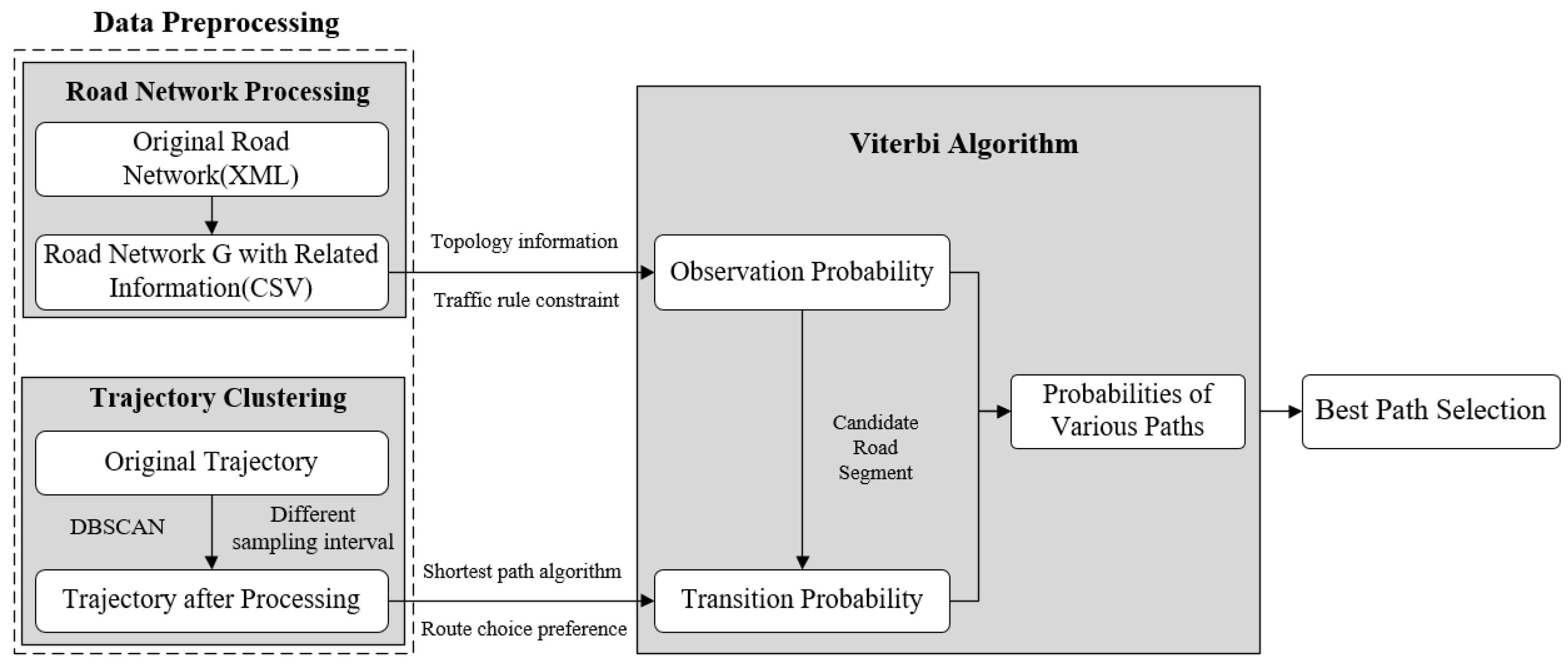
3.2. Algorithm Overview

The proposed algorithm is designed to select the best matched road segment for each GPS trajectory point. Figure 1 shows the architecture of our algorithm, which consists of two parts: data preprocessing and the construction of HMM.

• Part 1: data processing

This part contains two steps: trajectory clustering and road network processing. The GPS trajectory data were collected from dozens of volunteers in step 1. In the process of data integration and cleansing, converting the raw data into a format that allows for data mining. After that, the DBSCAN clustering algorithm is used to exclude the redundant trajectory points to improve the matching efficiency.

In the step of road network processing, the original road network, which presented in XML, is easily used to send data but has poor availability. By extracting relative information from the original file, standard road network can be established. Except the typical component of road network G, it also includes other elements, such as the road class, one-way road or not, the road’s name, the length and orientation of a road segment, that can be used in later procedure.

After the above data processing operations, the data suitable for the subsequent model construction are prepared.

• Part 2: Hidden Markov Model

Firstly, the network topology information obtained previously is used to calculate the observation probability. Secondly, the shortest path algorithm is applied to measure the shortest path and distance between candidate segments of time $i$ and $i+1$, and then the transition probability is computed. Lastly, HMM is used to calculate the probabilities of various inferred paths corresponding to track T, and the route with the highest probability is chosen as the optimal route.

• In summary, the overall flow of the proposed algorithm is as follows.

  (1)

  Input: Road network $G(V,E)$, each road segment $(lon,lat)\in E$ is associated with a list of properties, such as road ID, name, the start and end node, grade, speed limit, azimuth and a sequence of N observations $o_{1:N}=\{o_1,\cdots ,o_n\}$;

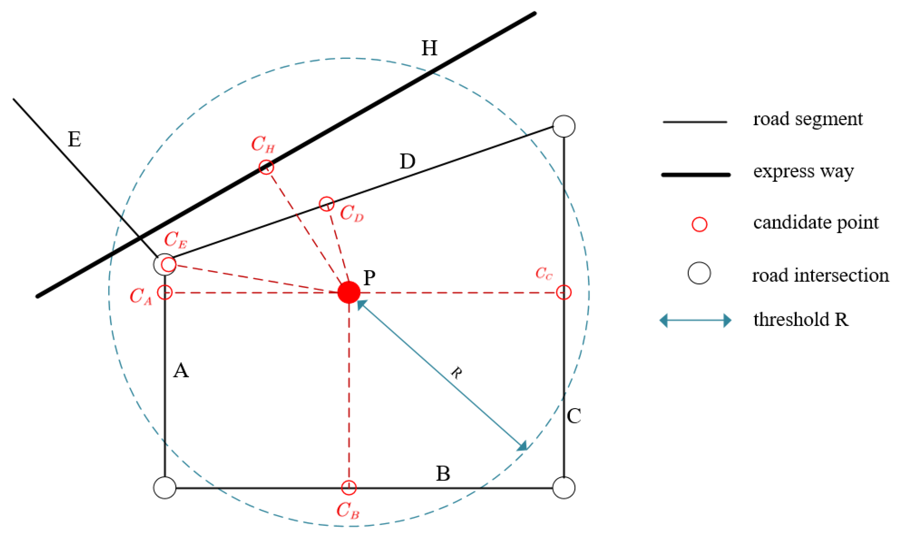
  (2)

  For a threshold value $R$, set the road segments within the proximity of observation $t(t=1,2,\mathrm{\dots }N)$ as the candidate links, as shown in Figure 2. Then, the observation probability for each candidate link is calculated;

  (3)

  When $t=1$, $V_{1,k}=p(o_1|s_{1,k})$ is treated as the initial state;

  (4)

  When $t=2,\mathrm{\dots }N$, the Viterbi algorithm $V_{t,k}=p(o_t|s_{t,k})·{\max }_j(V_{t-1,}{}_{j}p(s_{t,k}|s_{t-1,j}))$ is used to compute the state at time step $t$;

  (5)

  At the last time step $t=N$, the path with the highest probability is taken as the optimal path.

The following subsections present details of these steps.

3.3. Data Processing and Description

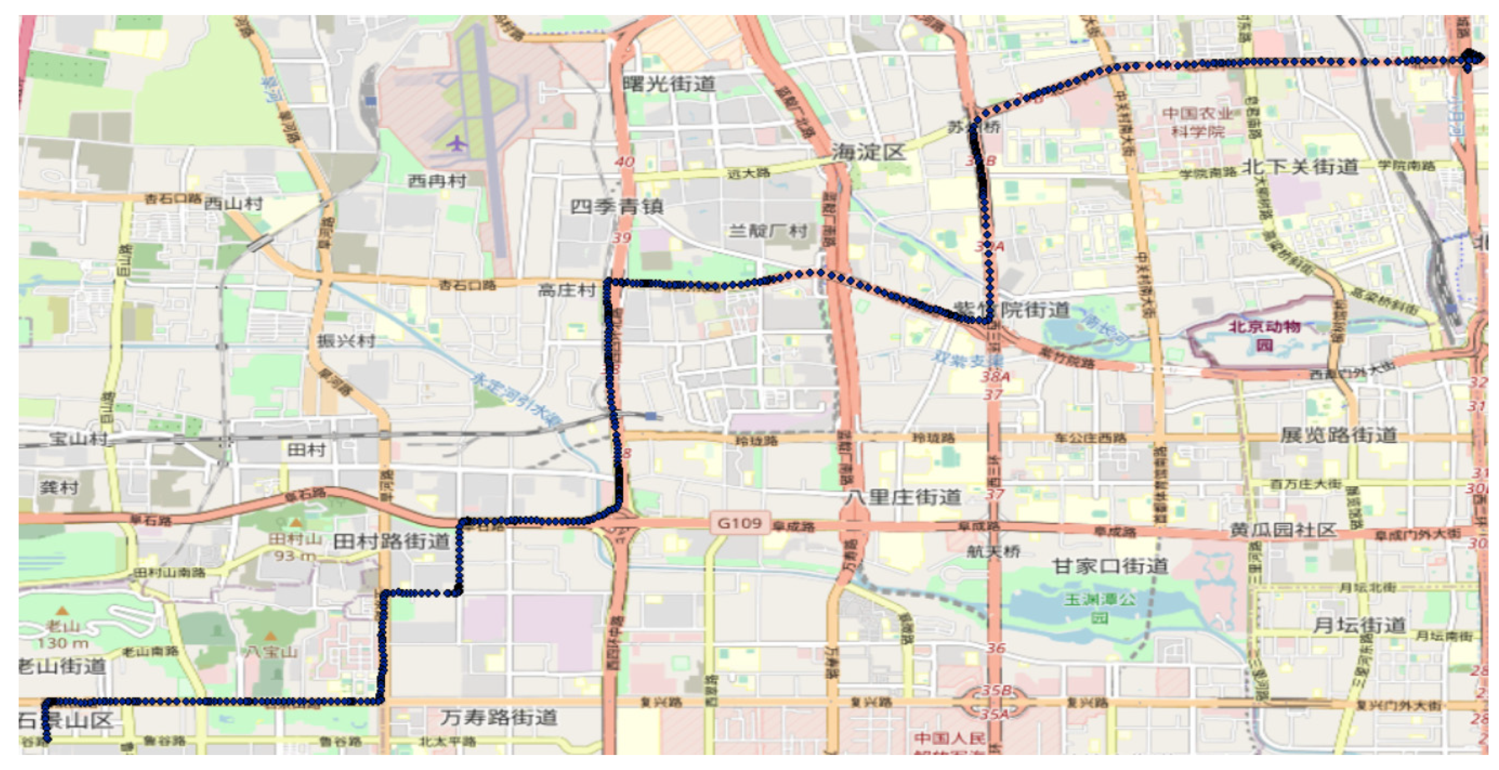
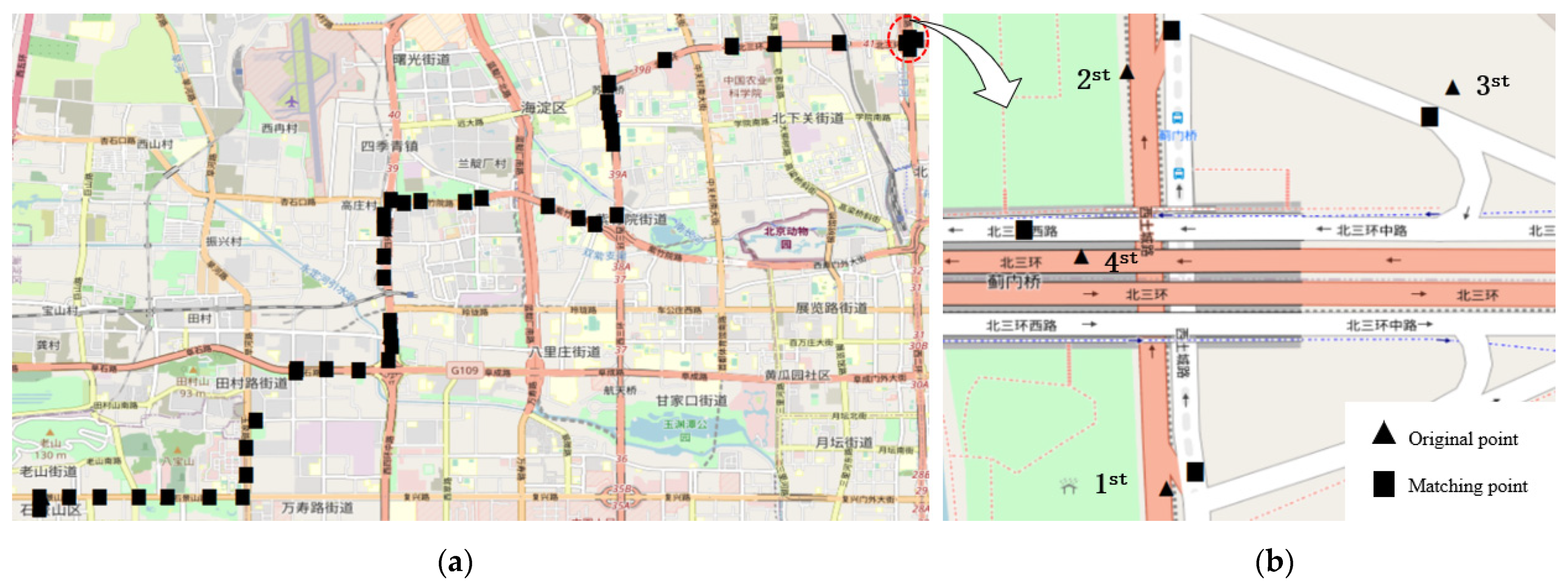
3.3.1. GPS Trajectory Data

In 2019, we employed about 60 volunteers to record GPS trajectory data of their daily activities while using a vehicle. Each observation point contains five fields: volunteer ID, time, longitude, latitude and speed, as shown in

Table 1. Sample from original trajectory data.

Volunteer ID	Time	Longitude	Latitude	Speed
1	25 February 2019 17:12:42	116.348533844	39.9656527041	10.73298
1	25 February 2019 17:12:49	116.348587135	39.9658000376	12.62736
1	25 February 2019 17:12:53	116.34855805	39.9659548095	15.11853
1	25 February 2019 17:12:58	116.348499544	39.9658969324	16.44845
1	25 February 2019 17:13:03	116.348489402	39.9658808811	14.98515
1	25 February 2019 17:13:08	116.348543298	39.9659085414	13.42683

. The sampling frequency is 5 s, and the total size is more than 80,000 pieces of records collected from 196 trips. Since this paper addresses the sparse data map matching problem, certain GPS points are removed from the original dataset, and datasets with sampling intervals of 30, 45 and 60 s are generated.

Different types of data problems such as data loss or data duplication often occur due to human negligence, equipment anomalies and other factors [13]. Direct analysis of these problematic data will produce erroneous or meaningless results and must be corrected through a process of data integration and cleansing prior to building data mining models.

After integrating and cleaning the original data, the next operation is to filter the dense track points using clustering. For two consecutive trajectory points, when the speed is very low, the distance will be too small to affect the subsequent map matching process. In this procedure, DBSCAN is applied to exclude dense points.

After data sampling, integration and cleansing and clustering, one volunteer trajectory will only contain several tens of geographic coordinates after preprocessing, just as Figure 3 illustrates.

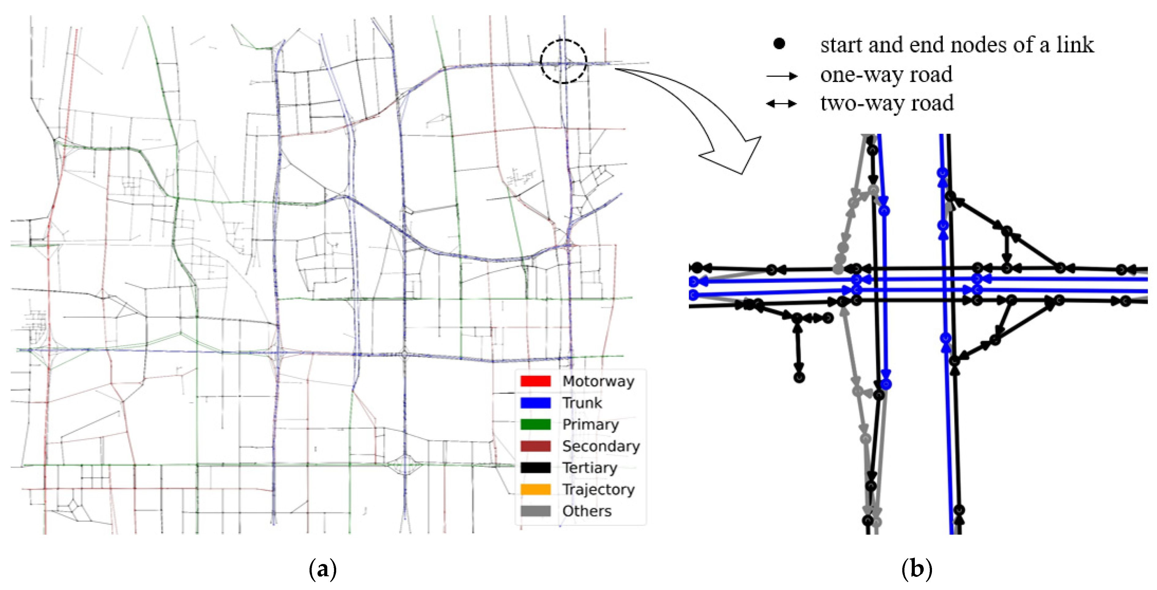
3.3.2. Road Network Data

We download the urban data of Beijing from OpenStreetMap, a website that aims to create and provide free geographic data, such as street maps, to anyone [14]. The original data file represents physical features on the ground (e.g., roads or buildings) using tags attached to their basic data structures, including nodes, ways and relations. The main attributes include the longitude and latitude of a node, the sequence of connecting nodes in a way, the ID and other tags of way, such as the name, if it is a highway and one-way or not.

Firstly, in order to construct the road network of Beijing, we need to extract information from label ways that equal highways. In detail, a highway has labels including “motorway”, “trunk”, “primary”, “secondary”, “tertiary”, “unclassified”, “motorway_link”, “trunk_link”, “primary_link”, “secondary_link”, “tertiary_link” that are selected in our work, for only the above types of roads are suitable for vehicles. Secondly, a way composited by ordered nodes is knitted, the name and one-way or not is also recorded in this step. Then, according to the Road Speed Limit Regulations of Beijing, the maximum speed is set for various roads. Finally, the length and bearing of the selected road is computed based on its longitude and latitude.

The selected road network contains 10,545 road segments and 9188 points. Apart from the linking sections, the average length of road segment is 91.54 m. Figure 4 presents the actual scene of the experiment and the display of the original trajectory data on the map of this paper. Figure 5 shows the basic structure of the road network that we extracted.

It should be noted that the OSM road network data were accessed in 2021, while the GPS trajectory data were collected in 2019. There is no big change in the road network from 2019 to 2021 in Beijing, particularly within the central part, where the data we collected. Minor changes in road networks would significantly affect the matching results, so better results could be anticipated if high-quality road network data are available.

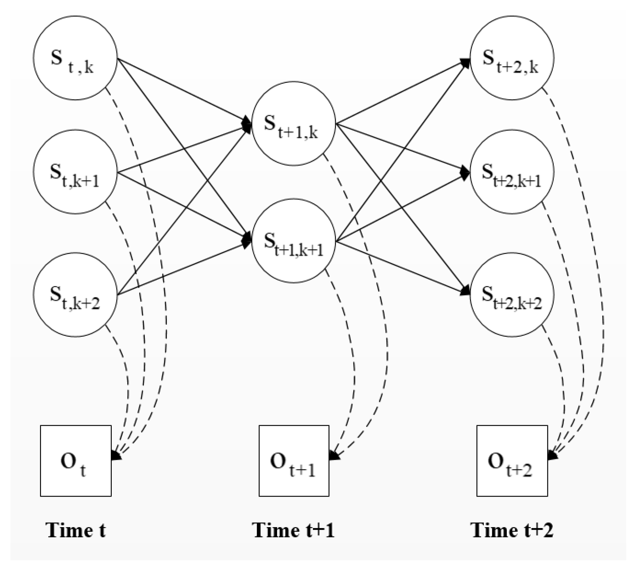
3.4. HMM in Map Matching

A Hidden Markov Model is a type of Markov Chain, which is defined as “A stochastic model describing a sequence of possible events in which the probability of each event depends only on the state attained in the previous event” [15]. It is useful in events in which one is interested but may not be directly observable in the world. In the field of map matching, an HMM models a system assumed to be a Markov process with unobservable states and observable observations [16].

In general, an HMM has the following two assumptions [17]:

• Markov Assumption: The probability of a particular state is dependent only on the immediate previous state:

$$p(s_t|s_1,o_1,\cdots ,s_{t-1},o_{t-1})=p(s_t|s_{t-1})\hspace{1em}t=1,2,\cdots ,T$$

• Independent Assumption: The probability of an observation $o_t$ is dependent only on the state that produced the observation $S_i$ and not on any other state or any other observations:

$$p(o_t|s_1,o_1,\cdots ,s_{t-1},o_{t-1},s_{t+1},o_{t+1},\cdots ,s_T,o_T)=p(o_t|s_t)$$

Figure 6 illustrates the model used. For a hidden state point $S_t$ at time step $t$, we can obtain the corresponding observation point $o_t$ with observation probability $b_t$. This state point could transfer to the next hidden state point $S_{t+1}$ with a transition probability ${\mathrm{a}}_{t+1}$. At first, it should have an initial state $\pi$, which denotes the probabilities of being in various states of the start time. Transition probability A, observation probability B and initial state probability vector $\pi$ are called the three elements in HMM [18].

In an HMM, there could be multiple sequences of states that are consistent with a given sequence of observations. The most likely state sequence can be efficiently calculated using the Viterbi algorithm [19]. The following introduces the workflow of this part.

3.4.1. Transition Probability

The transition probability between a state $S_{t–1,j}$ at time step $t–1$ and another state $S_{t,k}$ at time step $t$ depends on the features of the optimal path between them. For example, two candidates who lie on the same or consecutive road segment are more likely than on a parallel one, for it is unlikely that the object jumps from one road to the other across two sequential observations. Meanwhile, the road level of the candidate segments will not differ greatly.

In this paper, the path with the minimum free-flow travel time [20] and the difference in road class between the candidate road segments are considered as the main influence factors. This is calculated by assuming that the Euclidean distance between two candidates should be similar to the road-network distance between them. Haversine formula [21] is used to calculate the distance of two points, and Dijkstra’s algorithm [22] is applied when searching for the shortest path distance in road network between two candidates.

Firstly, we consider a temporal implausibility in order to allocate low transition probabilities to paths that are not possible within the time $\Delta T$ unless driving exceeds the speed limit. It defined as follows:

$$p_{time}=\frac{\max (T_{free}-\Delta T,0)}{\Delta T}$$

(1)

where:

$T_{free}$ = the free-flow travel time in seconds;

$\Delta T$ = the time interval between time steps $t+1$ and $t$ in seconds.

Generally, the shortest path distance between two candidate points at time step $t+1$ and $t$ is usually consider the most important factor [23], which is defined as the following distance variance probability:

$$p_D=\frac{1}{{\beta }_D}{e}^{-\frac{di{s}_{dif}}{{\beta }_D·\Delta T}}$$

(2)

$$di{s}_{dif}=|D_r-D_e|$$

(3)

$$\begin{array}{l}D=2R\ast \arcsin (\sqrt{hav({\varphi }_B-{\varphi }_A)-\cos ({\varphi }_A)\cos ({\varphi }_B)hav(L_B-L_A)}\\ \hspace{1em}=2R\ast \arcsin (\sqrt{{\sin }^2(\frac{{\varphi }_B-{\varphi }_A}{2})+\cos ({\varphi }_A)\cos ({\varphi }_B){\sin }^2(\frac{L_B-L_A}{2})}\end{array}$$

(4)

here:

$D_r$, $D_e$ are the shortest path distance and Euclidean distance of two candidate points, respectively;

${\beta }_D$ = the parameter of the exponential distribution;

$R$= the radius of the Earth;

${\varphi }_A,{\varphi }_B$ are the latitude of point 1 and point 2 (in radians), respectively;

$L_A,L_B$ are the longitude of point 1 and point 2 (in radians), respectively.

In addition to the topological information of the path, it is also important to consider the path selection habits of the driver [20]. In this part, we use a logit model to estimate the driver’s preference and consider all drivers to be identical as follows:

$$p_{choice}=\frac{e^{{\beta }_{{\chi }_{{}_i}}}}{{\displaystyle {\sum }_{p_j\in C}{e}^{{\beta }_{{\chi }_j}}}}$$

(5)

$$V_i={\beta }_i{\chi }_i={\beta }_{arc}{\chi }_{arc}+{\beta }_{nce}{\chi }_{nce}$$

(6)

where:

${\chi }_{arc},{\beta }_{arc}$ are the average road class and its parameter for the candidate route, respectively;

${\chi }_{nce},{\beta }_{nce}$ are the number of class changes and their parameters for the candidate route, respectively.

Therefore, the transition probability can be defined as follows:

$$p(s_t|s_{t-1})=p_{time}·p_D·p_{choice}$$

(7)

3.4.2. Observation Probability

The observation probability is the likelihood of each candidate point for a GPS point belonging to that point. For example, a candidate road segment closer to the raw observation point would have a higher measurement probability than one that is further away.

Similar to previous studies, the observation probability model refers only to the current candidate point and the observation point [24]. In this paper, observation probability is determined by distance, bearing deviation and speed constraint rules between observation and candidate road segments. In addition, we regard the point closest to the observation on the road segment as the candidate point.

As in previous studies, we treat the shortest distance between a trajectory point and a candidate road segment as the most important factor and define it as the distance constraint probability. In the case of the true state, the distance between itself and the observed location is the location measurement error, which is generally assumed to follow a Gaussian distribution with zero mean. The distance constraint probability is computed as follows:

$$p_{dis}=\frac{1}{\sigma \sqrt{2\pi }}{e}^{-\frac{di{s}^2}{2{\sigma }^2}}$$

(8)

$$\begin{array}{l}dis=2R\ast \arcsin (\sqrt{hav({\varphi }_B-{\varphi }_A)-\cos ({\varphi }_A)\cos ({\varphi }_B)hav(L_B-L_A)}\\ \hspace{1em}=2R\ast \arcsin (\sqrt{{\sin }^2(\frac{{\varphi }_B-{\varphi }_A}{2})+\cos ({\varphi }_A)\cos ({\varphi }_B){\sin }^2(\frac{L_B-L_A}{2})}\end{array}$$

(9)

where:

$dis$ = the great circle distance of two candidate points.

It is worth noting that, in practice, the location measurement error may not strictly conform to the above model, especially in dense urban networks. Irrespective of the positioning technology used, the error is known to exhibit non-Gaussian characteristics and geographical variations. However, the model based on Gaussian distribution, though simple, has been shown to be effective in several previous works on map matching [25].

In addition to the distance constraint, the azimuth difference is another important factor to be considered, which is defined as the azimuth constraint probability. The bearing $\theta$ of node A is the angle between the North and the direction to the next node B on the route. The value can be calculated with the following haversine formula:

$$p_{azi}=|\cos ({\theta }_{obs}-{\theta }_{candi})|$$

(10)

$$\theta =\arctan 2(\sin (L_B-L_A)\cos ({\varphi }_B)\cos ({\varphi }_A)\sin ({\varphi }_B)-\cos (L_B-L_A)\sin ({\varphi }_A)\cos ({\varphi }_B))$$

(11)

where:

${\theta }_{obs}$ = the instantaneous bearing of the observation point;

${\theta }_{candi}$ = the azimuth of the candidate road segment.

Finally, considering traffic rules, such as the speed of a vehicle cannot exceed the speed limit, traffic speed constraint probability is defined as follows:

$$p_{spe}=\{\begin{array}{l}1,\hspace{1em}{\alpha }_{spe}\le {\alpha }_{spe}\\ 0,\hspace{1em}{\alpha }_{spe}>{\alpha }_{spe}\end{array}$$

(12)

where:

${\alpha }_{spe}$ = the instantaneous velocity of the observation point;

${\alpha }_0$ = the maximum speed limit of candidate road.

Therefore, the observation probability can be introduced as follows:

$$p(o_t{|\mathrm{s}}_t)=p_{dis}·p_{zai}·p_{spe}$$

(13)

3.4.3. Viterbi Algorithm

The Viterbi algorithm takes the series of hidden states (candidate points) along with their associated measurement or transition probabilities as inputs. The first matched point is found simply as the candidate with the highest observation probability, as there are no transition probabilities for this base case. After this, the sets of candidates (for each GPS point) are iterated through and the candidate with the highest combination of measurement and transition probability is selected, considering only the observation transitions to the previous candidate points as per the Markov assumption.

It calculates the most probable sequence in the HMM using the following recurrence formulas:

$$\{\begin{array}{l}{V}_{1,k}=p(o_1|s_{1,k})\\ V_{t,k}=p(o_t|s_{t,k})·{\max }_j(V_{t-1}·p(o_{t,k}|s_{t-1,j}))\end{array}$$

(14)

where:

$p(o_t|s_{t,k})$ = the observation probability at time step $t$;

$p(s_{t,k}|s_{t-1,j})$ = the transition probability from time step $t–1$ to $t$;

$V_{t,k}$ = the maximum probability among all paths at time step $t$ when selecting candidate link $k$.

4. Experiments and Results

4.1. Parameter Setting

4.1.1. Maximum Distance

In the process of MM, road segments with a distance less than the maximum distance from the GPS trajectory point will be selected as a candidate link, and those with a greater distance will be excluded. In previous research results, the maximum distance is determined by the measurement error and standard deviation of an observation.

The measurement error ${\epsilon }_m$, which influences the efficiency and accuracy of map matching, includes trajectory point positioning errors and road data errors. $\epsilon$ is represented by Equation (15):

$${\epsilon }_m={\epsilon }_p+{\epsilon }_r$$

(15)

where:

${\epsilon }_p$ = positioning error; here, we take its value as 20 m;

${\epsilon }_r$ = road data error.

${\epsilon }_r$ is mainly caused by the difference between the actual road width and the road line data, and its calculation is as shown in Equation (16) [26]:

$${\epsilon }_r=0.5·\frac{w}{\sin \frac{\alpha }{2}}$$

(16)

where:

$w$ = the width of road, and the value of 40 m is taken here, which is approximately the width of eight lanes in both directions;

$\alpha$ = the angle between two intersecting roads. In order to simplify the calculation, the angle is generally considered to be 90 degrees.

In a normal distribution, 95% of the data fall within three standard deviations that are taken as 7.6 m [27], as follows:

$$3·{\sigma }_d=7.6m$$

According to the above influencing factors, the maximum distance is finally determined to be 50 m.

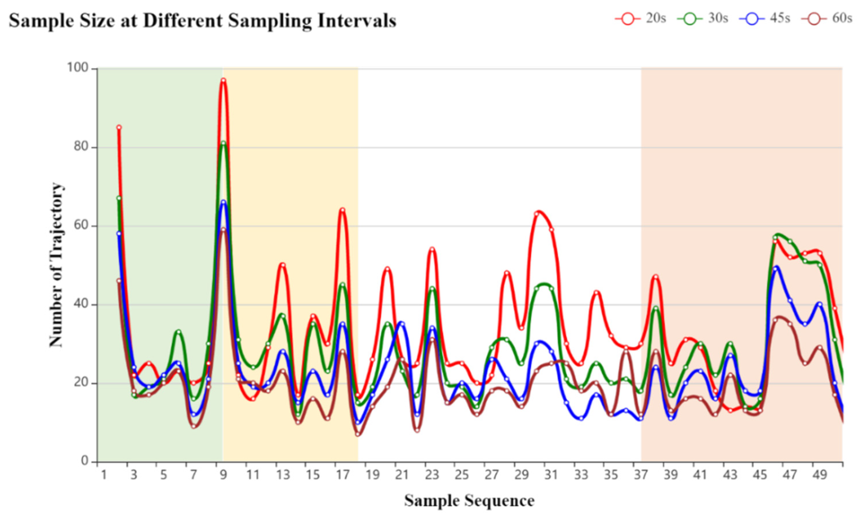
4.1.2. Parameters of the DBSCAN

DBSCAN is a density-based clustering algorithm: Given a set of points in some space, it combines those points that are closely aligned together and marks those points that lie individually in low-density regions as outliers. It requires two parameters: $\epsilon$ indicates the maximum distance of a neighborhood, and $MinPts$ describes the minimum number of points required to form a dense neighborhood [28].

In the prepared road network, excluding the connecting roads, the average length of the road segments is about 90 m. To construct a sparse trajectory, $MinPts$ is set to 3 and $\epsilon$ takes twice the average length of the section as 180 m to ensure that the contiguous observation points do not correspond to adjacent sections.

4.2. Assessment Criteria

In order to perform a comprehensive evaluation of the proposed algorithm, two evaluation metrics are used for comparison, including one accuracy criteria and one criterion related to the computation time.

The first is the accuracy ratio of matched points (AR), defined as follows [29,30]:

$$AR=\frac{{\displaystyle \sum _1^{T}C{N}_k}}{{\displaystyle \sum _1^T{N}_k}}$$

(17)

where:

$C{N}_k$ = the number of points matched to the correct road segment in trajectory $k$;

$N_k$ = the total number of points in trajectory $k$;

$T$ = the number of trajectories.

The second measurement criterion is the average time consumption for per trajectory point (AT), which is defined as follows:

$$ATC=\frac{{\displaystyle \sum _1^{T}T{C}_k}}{{\displaystyle \sum _1^T{N}_k}}$$

(18)

where:

$T{C}_k$ = the time consumption of trajectory $k$.

4.3. Results

As mentioned above, we compared the performance of the three algorithms at three sampling intervals of 20, 30, 45 and 60 s. The overall and partial results before and after map matching with a sampling interval of 120 s are shown in Figure 7, and the measurement results with variable sampling intervals are presented in

Table 2. Performance of the shortest path-based HMM algorithm with different sampling intervals.

Variables	Sampling Interval (s)
	20	30	45	60
Sample size	8332	6748	5612	4825
AR (%)	93.52	92.78	92.12	91.79
AT (s)	8.16	8.65	8.78	8.82

.

In addition to self-comparisons at different sampling intervals, we also compare the quality of the proposed shortest path-based HMM algorithm with two benchmark MM algorithms: a shortest path-based map matching algorithm (SPM) [4] and the HMM map matching algorithm (HMM) described in [31], using the dataset described in 3.3. The results of the experiment are shown in Figure 8.

According to Table 2 and Figure 8, we can draw the following conclusions:

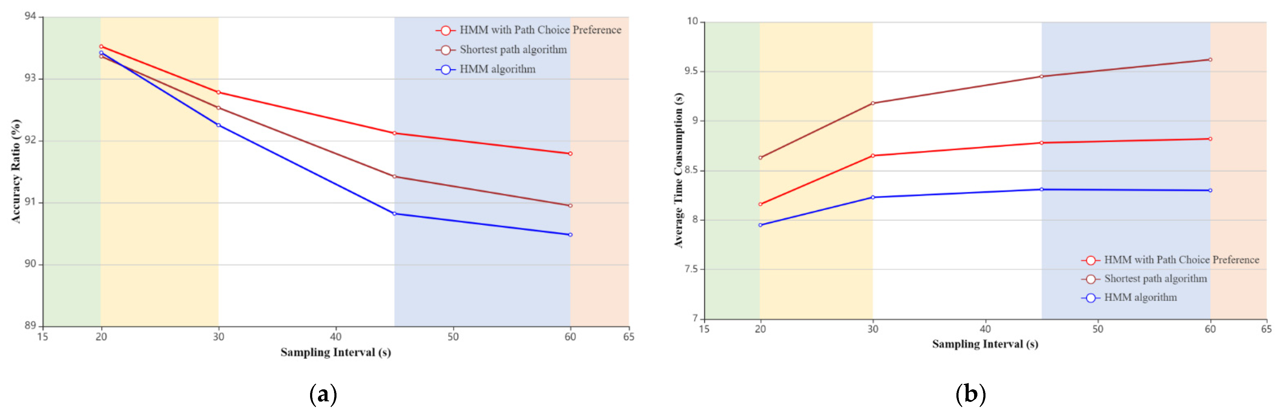
• As shown in Table 2, the accuracy ratio of matching decreases rapidly, and the average time consumption increases slowly when the sampling interval is increased. For the measurement of AT, when a larger sampling interval is selected, the amount of map data used to calculate the shortest path between adjacent trajectory points does not change much, resulting in constant average time consumption. Furthermore, when examining the mismatched points, we found that most of the mismatches occurred because the traveler did not choose the shortest path, which was inconsistent with our hypothesis and resulted in lower matching accuracy at larger sampling intervals.
• Figure 8a shows the matching accuracy of the three algorithms for four different sampling intervals, the horizontal axis represents the sampling frequency and the vertical axis represents the percentage of accuracy. The AR values of all three methods are higher than 0.9, while the proposed algorithm has higher matching accuracy than the other two. We also note that all three algorithms can achieve good matching precision at high frequency sampling, and the shortest path-based HMM performs better than the HMM and shortest path algorithms when the sampling frequency is low.
• In Figure 8b, the HMM algorithm has the smallest ATC for all four sampling intervals and the longest average time consumed by the SPM algorithm. On the other hand, when the sampling interval is greater than 30 s, the proposed algorithm and the HMM algorithm generate relatively stable ATC, while the ATC of the SPM algorithm gradually increases.

In summary, the proposed algorithm has higher matching precision than the two compared benchmark algorithms, especially when the trajectory points have a lower sampling frequency. However, its average time consumption is between the two algorithms, which is not satisfactory.

5. Conclusions and Discussions

In the paper, we propose a new map matching algorithm by integrating the HMM methods with the path choice preference. As the traditional shortest path-based MM algorithm for sparse trajectories, we first assume that the decision maker will choose the shortest path to travel between two candidate points. Furthermore, as with typical HMM-based algorithms, geometric topology information was applied, which includes both velocity constraints and time constraints. However, in addition to these strategies adopted above, the path selection preferences of drivers were also taken into account in this paper. This approach, which are better fit with the actual scene, can significantly increase matching efficiency without introducing excessive time consumption.

Based on real GPS trajectory data in Beijing, extensive experiments were conducted to verify the matching performance of the proposed algorithm. The experimental results show that when the sample interval is larger than 30 s, the proposed method improves the matching accuracy by 1% compared to the two benchmark algorithms. Although the algorithm can significantly improve the precision of map matching, its matching efficiency is slightly reduced, especially in the condition of sparse trajectory data. Without considering the time cost, the approach can help transportation researchers and practitioners process GPS track datasets more efficiently to match their own GIS data.

The matching efficiency of the proposed algorithm is not entirely satisfactory, and we guess that it consumes too much time using the shortest path strategy. Furthermore, there are situations where decision makers face more options when making path choices than just considering the shortest path and simple path selection preferences. Future research can explore more matching strategies to address these shortcomings and to improve the efficiency of matching and the plausibility of assumptions.

References

- Bernstein, D.; Kornhauser, A. An Introduction to Map Matching for Personal Navigation Assistants. 1998. Available online: https://rosap.ntl.bts.gov/view/dot/38257 (accessed on 16 November 2021).
- Militino, A.F.; Ugarte, M.D.; Iribas, J.; Lizarraga-Garcia, E. Mapping GPS positional errors using spatial linear mixed models. J. Geod. 2013, 87, 675–685. [Google Scholar] [CrossRef]
- Rahmani, M.; Koutsopoulos, H.N. Path inference from sparse floating car data for urban networks. Transp. Res. Part C Emerg. Technol. 2013, 30, 41–54. [Google Scholar] [CrossRef]
- Quddus, M.; Washington, S. Shortest path and vehicle trajectory aided map-matching for low frequency GPS data. Transp. Res. Part C Emerg. Technol. 2015, 55, 328–339. [Google Scholar] [CrossRef] [Green Version]
- Chen, B.Y.; Yuan, H.; Li, Q.; Lam, W.H.K.; Shaw, S.-L.; Yan, K. Map-matching algorithm for large-scale low-frequency floating car data. Int. J. Geogr. Inf. Sci. 2013, 28, 22–38. [Google Scholar] [CrossRef]
- Newson, P.; Krumm, J. Hidden Markov map matching through noise and sparseness. In Proceedings of the 17th ACM SIGSPATIAL International Conference on Advances in Geographic Information Systems, Seattle, WA, USA, 4 November 2009; pp. 336–343. [Google Scholar]
- White, C.E.; Bernstein, D.; Kornhauser, A.L. Some map matching algorithms for personal navigation assistants. Transp. Res. Part C Emerg. Technol. 2000, 8, 91–108. [Google Scholar] [CrossRef]
- Pyo, J.S.; Shin, D.H.; Sung, T.K. Development of a map matching method using the multiple hypothesis technique. In Proceedings of the ITSC 2001, 2001 IEEE Intelligent Transportation Systems, (Cat. No.01TH8585), Oakland, CA, USA, 25–29 August 2001; pp. 23–27. [Google Scholar]
- Bierlaire, M.; Chen, J.; Newman, J. A probabilistic map matching method for smartphone GPS data. Transp. Res. Part C Emerg. Technol. 2013, 26, 78–98. [Google Scholar] [CrossRef]
- Luo, A.; Chen, S.; Xv, B. Enhanced Map-Matching Algorithm with a Hidden Markov Model for Mobile Phone Positioning. ISPRS Int. J. Geo-Inf. 2017, 6, 327. [Google Scholar] [CrossRef] [Green Version]
- Lou, Y.; Zhang, C.; Zheng, Y.; Xie, X.; Wang, W.; Huang, Y. Map-matching for low-sampling-rate GPS trajectories. In Proceedings of the 17th ACM SIGSPATIAL International Conference on Advances in Geographic Information Systems, Seattle, WA, USA, 4 November 2009; pp. 352–361. [Google Scholar]
- Hsueh, Y.-L.; Chen, H.-C. Map matching for low-sampling-rate GPS trajectories by exploring real-time moving directions. Inf. Sci. 2018, 433–434, 55–69. [Google Scholar] [CrossRef]
- Zheng, Y. Trajectory Data Mining. ACM Trans. Intell. Syst. Technol. 2015, 6, 1–41. [Google Scholar] [CrossRef]
- OpenStreetMap. Available online: https://wiki.osmfoundation.org/wiki/Main_Page (accessed on 15 September 2021).
- Dogramadzi, M.; Khan, A. Accelerated Map Matching for GPS Trajectories. IEEE Trans. Intell. Transp. Syst. 2021, 1–10. [Google Scholar] [CrossRef]
- Rabiner, L.R. A tutorial on hidden Markov models and selected applications in speech recognition. Proc. IEEE 1989, 77, 257–286. [Google Scholar] [CrossRef]
- Yu, S.-Z. Hidden semi-Markov models. Artif. Intell. 2010, 174, 215–243. [Google Scholar] [CrossRef] [Green Version]
- Rabiner, L.; Juang, B. An introduction to hidden Markov models. IEEE ASSP Mag. 1986, 3, 4–16. [Google Scholar] [CrossRef]
- Luo, L.; Hou, X.; Cai, W.; Guo, B. Incremental route inference from low-sampling GPS data: An opportunistic approach to online map matching. Inf. Sci. 2020, 512, 1407–1423. [Google Scholar] [CrossRef]
- Jagadeesh, G.R.; Srikanthan, T. Online Map-Matching of Noisy and Sparse Location Data With Hidden Markov and Route Choice Models. IEEE Trans. Intell. Transp. Syst. 2017, 18, 2423–2434. [Google Scholar] [CrossRef]
- Sinnott, R. Virtues of the Haversine. Sky Telesc. 1984, 68, 158. [Google Scholar]
- Dijkstra, E.W. A note on two problems in connexion with graphs. Numer. Math. 1959, 1, 269–271. [Google Scholar] [CrossRef] [Green Version]
- Chambers, E.; Fasy, B.T.; Wang, Y.; Wenk, C. Map-Matching Using Shortest Paths. ACM Trans. Spat. Algorithms Syst. 2020, 6, 1–17. [Google Scholar] [CrossRef] [Green Version]
- Liu, M.; Zhang, L.; Ge, J.; Long, Y.; Che, W. Map Matching for Urban High-Sampling-Frequency GPS Trajectories. ISPRS Int. J. Geo-Inf. 2020, 9, 31. [Google Scholar] [CrossRef] [Green Version]
- Hunter, T.; Abbeel, P.; Bayen, A. The Path Inference Filter: Model-Based Low-Latency Map Matching of Probe Vehicle Data. IEEE Trans. Intell. Transp. Syst. 2014, 15, 507–529. [Google Scholar] [CrossRef] [Green Version]
- Qi, H.; Di, X.; Li, J. Map-matching algorithm based on the junction decision domain and the hidden Markov model. PLoS ONE 2019, 14, e0216476. [Google Scholar] [CrossRef] [PubMed]
- Wikipedia. Error Analysis for the Global Positioning System. Available online: https://en.wikipedia.org/wiki (accessed on 21 September 2021).
- Sander, J.; Ester, M.; Kriegel, H.-P.; Xu, X. Density-Based Clustering in Spatial Databases: The Algorithm GDBSCAN and Its Applications. Data Min. Knowl. Discov. 1998, 2, 169–194. [Google Scholar] [CrossRef]
- Wu, Z.; Xie, J.; Wang, Y.; Nie, Y. Map matching based on multi-layer road index. Transp. Res. Part C Emerg. Technol. 2020, 118. [Google Scholar] [CrossRef]
- Miwa, T.; Kiuchi, D.; Yamamoto, T.; Morikawa, T. Development of map matching algorithm for low frequency probe data. Transp. Res. Part C Emerg. Technol. 2012, 22, 132–145. [Google Scholar] [CrossRef]
- Hu, Y.; Lu, B. A Hidden Markov Model-Based Map Matching Algorithm for Low Sampling Rate Trajectory Data. IEEE Access 2019, 7, 178235–178245. [Google Scholar] [CrossRef]