Evolutionary Game Analysis on Last Mile Delivery Resource Integration—Exploring the Behavioral Strategies between Logistics Service Providers, Property Service Companies and Customers

Abstract

As resource integration plays a significant part in improving operational efficiency in the last mile delivery industry, there is an increasing popularity for logistics service providers (LSPs) to collaborate with property service companies (PSCs). Based on the evolutionary game theory, considering the dual role of PSCs when collaborating with LSPs, a trilateral evolutionary game model between PSCs, LSPs, and customers (Cs) is established to analyze the strategic choices and explore the influencing factors on the tripartite strategy. The results show that (1) There are optimal profit allocation coefficients and cost-sharing coefficients to cause the system to reach a steady state. (2) The integration cost between LSPs and PSCs and the home delivery cost inhibit the strategic integration of the two enterprises. (3) PSCs are more sensitive to their benefits and costs than LSPs in the process of resource integration. (4) More precisely evaluating their potential loss caused by temporary integration will help the tripartite to make a more scientific choice of strategic behavior. (5) The increase of community premium income helps to improve the enthusiasm of Cs supporting strategic integration. (6) The behavior and decision-making choices of the three game players affect each other in the last mile delivery resource integration. (7) The indirect benefits, such as advertising during their integration, play a positive role. Finally, the MATLAB2020a software is applied to simulate and analyze the impact of key factors on strategy evolution, and we propose several useful suggestions to promote the development of last mile delivery resource integration.

1. Introduction

The growing popularity of online shopping has driven a surge in express logistics with the rapid development of e-commerce [1]. According to the latest data reported by the Ministry of Transport of China, the average annual growth rate of the express delivery business in the past five years has exceeded 30 percent in China and ranks the first position in the world. What is more, the per capita packages are nearly 60 in 2020, which is about twice as high as the global average. However, due to spatial decentralization of demands, as well as specific requirements of customers [2], last mile delivery is regarded as the most expensive but least efficient part of the e-commerce logistics [3]. With increasing competition among LSPs and growing expectations for quality and service from customers, last mile delivery is one of the largest challenges in business to customer e-commerce [4]. Thus, LSPs must develop efficient strategies to try to reduce costs when designing their last mile operation systems [5].

Resource integration or corporation with other firms enables LSPs to develop and maintain a competitive advantage as the increasing of the economics of scale and more effective assets utilization [5,6] has drawn wide consideration during past decades. Several types of corporation have appeared in the last mile delivery industry. One of the main choice is to perform joint delivery through the alliance among couriers [7]. Crowdsourcing delivery is another very popular choice. In 2018, Walmart began to pilot crowdsourcing distribution in two cities in the United States. There is an increasing number of courier crowdsourced delivery companies in reality, such as Dada, Jingdong crowdsourcing, Postmates, UberEats, PiggyBee, DHL MyWays, UberFreight, BuddyTruk, etc. These companies combine shippers with people who provide shared mobile services to achieve the goal, which provides more economical transportation services than traditional transportation modes by postal services or overpriced logistics companies [8].

Different to traditional city logistics, which provide only door-to-door delivery, LSPs should also provide pickup service as well for both operation cost reduction and customers’ requirements considerations. With the exception of construction-dedicated attendant or unattended facilities, in collaborating with convenience stores, PSCs, and other institutions, LSPs can obtain significant benefits by taking these places as collection-and-delivery points [9]. Among these institutions, PSCs play a crucial role in last mile delivery collaboration. As PSCs are located close to final customers, they can provide parcel collection and temporary storage service with their underutilized offices or the available community space which makes customers’ pickup more convenient. Moreover, as they provide property services every day, they may have the possibility to play a role in delivering packages to customers.

Although it is common in practice that couriers place packages in PSCs’ office and wait for customers’ pickups, this is usually personal behavior for couriers, instead of LSPs and PSCs who receive no pay. In such scenarios, potential conflicts among LSPs, PSCs, and customers may occur when service and package quality are not well guaranteed. When PSCs collaborate with LSPs to provide better service from a commercial perspective, extra investment will result and then PSCs play a dual role, simultaneously providing property and last mile delivery service. With these considerations, what kind of collaboration will LSPs and PSCs take? What is the Cs’ attitude towards the collaboration and what factors may affect the collaboration? These are interesting issues and there is no research focus on this problem, to the best of our knowledge.

In this study, with the aim of providing useful decision-making guidance for resource integration of the last mile delivery, and thus to help to improve the delivery efficiency, we develop an evolutionary game model with heterogeneous players. We first analyze the behavioral strategies of LSPs, PSCs, and Cs during the collaboration. Then, we use the evolutionary game model to analyze the evolutionary stable strategy (ESS) and explain how the dynamic interaction between LSPs, PSCs, and Cs influences the players’ behaviors, and why and how these groups achieve the equilibrium state. Subsequently, numerical simulations are conducted to illustrate the appropriate policies in different scenarios. At last, we provide some suggestions to promote resource integration of the last mile delivery.

The remainder of the paper is organized as follows. Section 2 reviews the relevant literature. Section 3 describes the issue and constructs a tripartite dynamic evolutionary game model among PSCs, LSCs, and Cs. Section 4 analyzes the evolution path of the game players. Section 5 discusses the sensitivity analysis of selecting parameters in detail. Finally, research conclusions and highlights related to managerial implications are given in Section 6.

2. Literature Review

As a means of optimizing resource allocation, resource integration has promoted the rapid development of the logistics industry. Samir et al. believe that logistics resource integration is an understanding from the perspective of the supply chain and enterprises, that is, related resources carry out a higher level of cooperation in order to meet social needs [10]. Daniel et al. believe that logistics resource integration is one of the four flow integrations of logistics, information, resources, and processes in the supply chain [11]. Therefore, in recent years, resource integration has been the important necessity in developing logistics and there have been numerous studies investigating resource integration by integrating the supply chain resources and cooperating the last mile delivery.

Panayides et al. studied the impact of logistics resource integration on the performance of third-party logistics services [12]. Xu et al. and Yao et al. respectively studied the optimization of logistics resource allocation from the perspective of logistics network and fourth-party logistics [13,14]. Cao et al. discussed the operation of supply chains from three aspects: supplier integration, internal integration, and consumer integration, and studied the integration process from three perspectives: logistics integration, information flow integration, and capital flow integration [15]. Shi et al. studied the manufacturing enterprises from the perspective of information resource integration of reverse logistics [16]. Fan et al. proposed an internal and external integrated supply chain logistics optimization model to reduce the total logistics cost [17]. Frank et al. discussed the coordination and integration of supply chain resources in increasing supply chain performance [18]. Fan et al. studied the coordination mechanism of port logistics resource integration from the perspective of supply and demand [19]. Kim et al. combined the viewpoint of resource dependence theory to evaluate the impacts of trust, satisfaction, and commitment on enterprise logistics integration decision-making, and also studied the relationship between logistics integration and supply chain performance [20]. Zhu et al. believe that object identifier plays a more and more important role in the integration of modern logistics resources [21]. Yin et al. found that integrating the nodes between supermarkets and commercial logistics distribution centers and production bases is of great significance to the development of commercial enterprises in China [22]. Chen et al. introduced the evaluation method of logistics network infrastructure of railway logistics enterprises from the perspective of logistics resource integration [23].

In order to satisfy customers’ personalized demand, the last mile delivery has to continue to develop. Yang et al. pointed out that collaborative distribution can solve the personalization of distribution time and reduce pollution to a certain extent [5]. The most attention has given to horizontal cooperation, defined by Cruijssen et al. [24], as “a cooperation between two or more firms that are active at the same level of the supply chain, and perform a comparable logistics function on the landside.” A typical scenario of horizontal cooperation of last mile delivery is joint or collaborative delivery. Cruijssen et al. performed joint route planning to provide empirical evidence on the level of cost savings; results showed that joint route planning can save 30.7% of total distribution costs [25]. Yang et al. proposed a cooperative game model for collaborative distribution between two logistics service providers, several profitable cooperation conditions, as well as useful suggestions are provided. He et al. proposed a genetic framework for the selection of the optimal location of the joint distribution center and developed a sustainable evaluation system [7]. Zhou et al. introduced a two-echelon-based joint distribution system and proposed a two-echelon vehicle routing problem to provide customers with different delivery options to address the challenges arising in the last mile delivery [26]. Wang et al. established a collaborative logistics pickup and delivery problem with eco-packages for city collaborative alliance [27]. Widespread application of horizontal cooperation of last mile delivery in China is the Cai Niao Courier Station in the Alibaba Group, which provides pickup service for the integrated packages from several couriers.

Moreover, growing attention has been given to crowdsourced delivery, where ordinary people or agents help to carry out last mile delivery tasks. Archetti et al. were the first to model the problem of the crowdsourced deliverers in logistics networks by modeling the vehicle routing problem with occasional drivers [28]. Chen et al. proposed an innovative solution to collect the e-commerce-returned goods by using taxis [29]. Kafle et al. studied a crowdsource-enabled system, in which pedestrians and/or cyclists complete the last leg of a delivery task, while a truck carries the rest of the delivery [30]. Devari et al. presented a scenario-based analysis of the benefits of crowdsourcing last mile delivery by exploiting a social network of the customers. Marcina et al. considered a crowd-shipping problem with transshipment nodes [31].

To sum up, the main gaps between this paper and the past literature are as follows: (a) To the best of our knowledge, existing studies explored the last mile delivery resource integration on an operational level, and few analyze the strategic perspective. In this paper, we develop an evolutionary game theory model to study the dynamic strategic behavior of stakeholders in the last mile delivery. (b) We focus on the dual roles of PSCs and Cs, and explore the behavioral strategies of PSCs, LSPs, and Cs during their collaboration in last mile delivery, which is a novel perspective.

3. Evolutionary Game Model

3.1. Problem Description and Game Strategy

With fierce competition in the market and the increasing customer demands for personalization, driven by reducing the operation cost and improving the delivery efficiency, LSPs expect to cooperate with PSCs to better carry out the last mile delivery service. The last mile delivery service provided by PSCs is an extension of their core business, and value-added services revenue can be obtained. In view of the dual identity of proprietor and logistics clients, Cs can obtain direct logistics service-level improvement and related benefits due to resource integration.

There are two typical strategies in last mile delivery cooperation between LSPs and PSCs: one is temporary integration (TI), the other is strategic integration (SI). LSPs temporarily rent facility resources of PSCs’ to provide Cs with collection and self-pickup services during temporary integration. In this situation, PSCs are economically sensitive to their input during the cooperation due to the lack of business stability. When performing strategic integration, LSPs and PSCs carry out in-depth cooperation in parcel collection, storage, and home delivery services. In addition, to seek a long-term win–win situation, LSPs and PSCs may both increase investment on the basis of TI to improve service capacity as well as realize the in-depth integration of services, processes, and information, and PSCs will share the cost with LSPs based on the principle of revenue sharing. Meanwhile, no matter what kind of integration strategy LSPs and PSCs take, due to dual identities of Cs’, they have two optional strategic behaviors towards to the integration of the two companies, namely supporting temporary integration (STI) and supporting strategic integration (SSI), and what attitude they will take depends on the benefits they obtain and their losses during the integration.

3.2. Model Assumptions and Profit Matrix

Based on previous analysis, LSPs, PSCs, and Cs, the three game players of this article, are bound by rationality and hope to maximize their own utility, and the strategy space of them is denoted as S_LSPs = {TI, SI}, S_PSCs = {TI, SI}, and S_Cs = {STI, SSI}, respectively. For constructing a game model of stakeholders in last mile delivery resource integration and studying the conflicts of interests and optimal choices among them, the following basic assumptions are given.

Assumption 1.

If both LSPs and PSCs adopt the TI strategy, LSPs will pay the parcel storage cost$C_1$to obtain the temporary storage and management service provided by PSCs, then PSCs will receive$C_1$and bear the parcel storage operating cost$C_2$. At this time, LSPs will gain the distribution income$M_1$due to the improvement of customer pick-up convenience. Meanwhile, Cs will receive the pick-up convenience profit$U$and the resource occupation compensation B (B <$C_1$) given by PSCs due to temporary occupation of the community public resources when providing temporary package storage.

Assumption 2.

Compared to temporary integration, the home delivery cost$C_3$is invested in strategic integration. If both LSPs and PSCs discover that SI strategy is selected,$C_3$will be shared by the two companies. However, if they choose different strategies,$C_3$is paid by the one adopting the SI strategy. In addition, they will share the integration cost$C_4$, as both parties need to deeply integrate their services, processes, and information when they both choose the SI strategy. It is assumed that$\alpha (0<\alpha <1)$is cost-sharing coefficient, and then LSPs and PSCs bear the cost$\alpha \left(C_3+C_4\right)$,$\left(1-\alpha \right)\left(C_3+C_4\right)$, respectively.

Assumption 3.

When both LSPs and PSCs adopt the SI strategy, Cs will receive the service quality improvement profit$\Delta U$based on pick-up convenience due to obtaining the services such as home delivery. Due to the improvement of customers’ satisfaction with last mile delivery service, delivery efficiency, package integrity, and customers’ loyalty to property service, LSPs and PSCs will gain the service benefit$\Delta M_1$,$\Delta M_2$, respectively. At the same time, they will also obtain the indirect income$R$, such as value-added services revenue, by advertising on express packaging or express service facilities. However,$R$will be obtained by the party adopting the SI strategy when the two companies hold different strategies. Supposing that$\beta (0<\beta <1)$is profit allocation coefficient, then LSPs and PSCs receive the income$\beta R$,$\left(1-\beta \right)R$, respectively.

Assumption 4.

When either LSPs or PSCs tend to the SI strategy, the distribution service profit$U_i\left(i=1,2\right)$is obtained by Cs. However, compared to both of the two parties taking the SI strategy, time flexibility for home delivery is insufficient when LSPs choose the SI strategy and PSCs the other, and the value of the service provided will be lower, where$U_1<U+\Delta U$. Similarly, when LSPs adopt the SI strategy and PSCs the other, due to the lack of accurate information support such as logistics information systems, the value of the services provided will be lower as well, where$U_2<U+\Delta U$. In addition, the party carrying out the TI strategy will have potential losses$S_i\left(i=1,2\right)$due to failure to improve the service level.

Assumption 5.

When Cs choose the STI strategy, they will bear the potential loss$S_3$, that is, compared to the cost they paid in choosing the current SSI strategy, they will pay more when they are more inclined to the service benefits brought about by the SI strategy in the future. When both of the two companies choose the SI strategy and Cs choose the SSI strategy, Cs will gain the community premium income K due to the improvement of logistics service levels on the basis of obtaining the distribution service income. At this time, Cs may give up the resource occupation compensation B to promote the strategic integration of the two enterprises in order to maximize their own interests. However, when LSPs and PSCs perform strategic integration, the advertising behavior and the construction of fixed delivery facilities will have a negative impact on the community living environment to a certain extent, and then this brings the living environment loss S to Cs.

Assumption 6.

We make x$\left(0\le x\le 1\right)$represent the probability of LSPs choosing the SI strategy, and$\left(1-x\right)$denotes the probability of choosing the TI strategy. For PSCs, suppose that the probability of choosing the SI strategy is$y\left(0\le y\le 1\right)$, the probability of TI is$\left(1-y\right)$. In addition, denote$z\left(0\le z\le 1\right)$and$\left(1-z\right)$as the probability of Cs with a choice of the SSI and STI strategy, respectively, where$x,y,z\in \left[0,1\right]$.

According to the abovementioned analysis and hypothesis, the game payoff matrix of LSPs, PSCs, and Cs is presented in

Table 1. Payoff matrix of players in dynamic game model.

LSPs	PSCs	Cs
		SSI	STI
SI	SI	$M_1+\Delta M_1+\beta R-\mathsf{\alpha }\left(C_3+C_4\right)$ $\Delta M_2+\left(1-\beta \right)R-C_2-\left(1-\mathsf{\alpha }\right)\left(C_3+C_4\right)$ $U+\Delta U+K-S$	$M_1+\Delta M_1+\beta R-C_1-\mathsf{\alpha }\left(C_3+C_4\right)$ $\Delta M_2+\left(1-\beta \right)R+C_1-C_2-\left(1-\mathsf{\alpha }\right)\left(C_3+C_4\right)-B$ $U+\Delta U+B-S-S_3$
	TI	$M_1+\Delta M_1+R-C_1-C_3$ $C_1-C_2-S_2-B$ $U_1+B-S$	$M_1+\Delta M_1+R-C_1-C_3$ $C_1-C_2-S_2-B$ $U_1+B-S_3-S$
TI	SI	$M_1-C_1-S_1$ $\Delta M_2+C_1+R-C_2-C_3-B$ $U_2+B-S$	$M_1-C_1-S_1$ $\Delta M_2+C_1+R-C_2-C_3-B$ $U_2+B-S-S_3$
	TI	$M_1-C_1-S_1$ $C_1-C_2-S_2-B$ $U+\mathrm{B}$	$M_1-C_1-S_1$ $C_1-C_2-S_2-B$ $U+B-S_3$

.

4. Evolutionary Stable Strategy Analysis

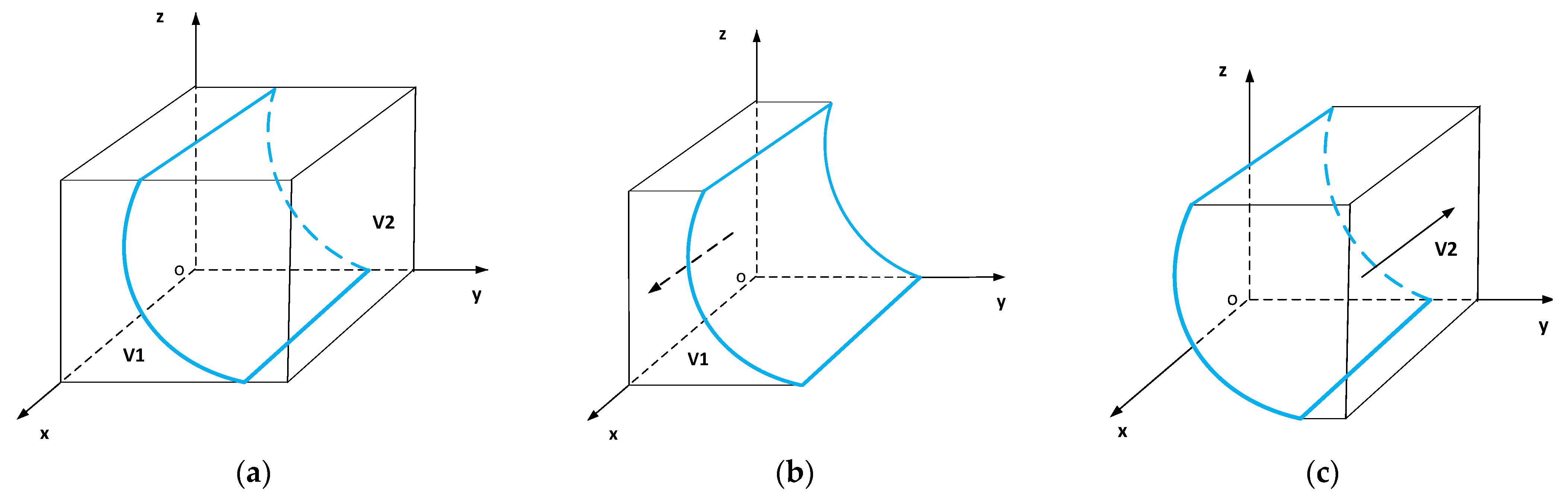
4.1. Strategy Stability Analysis of LSPs

According to the payoff matrix of the tripartite game, the expected payoffs of LSPs adopting the SI strategy and the TI strategy are described as follows, respectively.

$$\begin{array}{c}{U}_{L1}=yz\left(M_1+\Delta M_1+\beta R-\alpha \left(C_3+C_4\right)\right)+y\left(1-z\right)(M_1+\Delta M_1+\beta R-C_1-\alpha (C_3+\\ C_4))+\left(1-y\right)z\left(M_1+\Delta M_1+R-C_1-C_4\right)+\left(1-y\right)\left(1-z\right)(M_1+\Delta M_1+R-\\ C_1-C_3) \\ U_{L2}=yz\left(M_1-C_1-S_1\right)+y\left(1-z\right)\left(M_1-C_1-S_1\right)+\left(1-y\right)z\left(M_1-C_1-S_1\right)+(1-\\ y)\left(1-z\right)\left(M_1-C_1-S_1\right) \end{array}$$

Thus, the average expected payoff of LSPs is

$${\overline{U}}_L=x{U}_{L1}+\left(1-x\right)U_{L2}$$

The replicator dynamic equation for LSPs is as follows.

$$\begin{array}{c}F\left(x\right)=\frac{d_x}{d_t}=x\left(U_{L1}-{\overline{U}}_L\right) \\ =x\left(1-x\right)\left(y\left(-\left(1-\beta \right)R-\alpha \left(C_3+C_4\right)\right)+yz{C}_1+\Delta M_1+R+S_1\right)\end{array}$$

(1)

Therefore, we have the first derivative of the replicator dynamic equation of LSPs that can be obtained.

$$F^{\prime }\left(x\right)=\left(1-2x\right)\left(y\left(-\left(1-\beta \right)R-\alpha \left(C_3+C_4\right)\right)+yz{C}_1+\Delta M_1+R+S_1\right)$$

According to the Friedman method, when $F\left(x\right)=0$ and $F^{\prime }\left(x\right)<0$, x is an evolutionary stable strategy (ESS). Let $F\left(x\right)=0$; by calculating Equation (1), we can obtain that x = 1, x = 0, and $y_0=\left(-\Delta M_1-R-S_1)/(-\left(1-\beta \right)R-\alpha \left(C_3+C_4\right)+z{C}_1\right)$, and then proposition 1 is true.

Proposition 1 (1).

If$y=y_0$, then for any x,$F\left(x\right)\equiv 0$. That is, the probability of LSPs choosing the SI strategy is any value between 0 and 1.

Proposition 1 (2).

If$y\ne y_0$and$F\left(x\right)=0$, then the probability of LSPs choosing the SI strategy is x = 0 or x = 1.

Proof. 

Let $H\left(y\right)=\left(y\left(-\left(1-\beta \right)R-\alpha \left(C_3+C_4\right)\right)+yz{C}_1\right)+\Delta M_1+R+S_1-C_3$, $\partial H\left(y\right)/\partial \mathrm{y}<0$ can be obtained after calculation. Therefore, $H\left(y\right)$ is a decreasing function of y; when $y=y_0$, $H\left(y\right)=0$, $F\left(x\right)=0$, and $F^{\prime }\left(x\right)=0$, any production strategy of LSPs is a stable strategy, as shown in Figure 1a. While $y\ne y_0$, the following two cases are discussed further. □

(1)

If $0<y_0<y<1$, $H\left(y\right)>0$, ${F\left(x\right)|}_{x=1}=0$, and ${F^{\prime }\left(x\right)|}_{x=1}<0$, we can see x = 1 is the only ESS, and LSPs will adopt the SI strategy, as shown in Figure 1b.

(2)

If $0<y<y_0<1$, $H\left(y\right)<0$, ${F\left(x\right)|}_{x=0}=0$, and ${F^{\prime }\left(x\right)|}_{x=0}<0$, we can see x = 0 is the only ESS, and LSPs will adopt the TI strategy, as shown in Figure 1c.

Based on proposition 1, the replicator dynamics phase diagram of LSPs is shown in Figure 1.

As seen from Figure 1a, V1 represents the initial strategy set space that meets the condition $0<y_0<y<1$. When the numerical relationship between x and y corresponds to the space V1, SI is the evolutionary stable strategy of LSPs. Similarly, for V2, TI strategy is the evolutionary stable strategy. Therefore, the volumes $T_{V1}$ and $T_{V2}$ represent the probability that LSPs choose different strategies, which can be calculated as follows:

$$\begin{array}{c} T_{V1}=\underset{V1}{\overset{ }{{\displaystyle \iint }}}\frac{-\Delta M_1-R-S_1}{-\left(1-\beta \right)R-\alpha \left(C_3+C_4\right)+z{C}_1}dydz \\ =\frac{\Delta M_1+R+S_1}{C_1}ln\left(\frac{\alpha \left(C_3+C_4\right)+\left(1-\beta \right)R-C_1}{\alpha \left(C_3+C_4\right)+\left(1-\beta \right)R}\right) \\ T_{V2}=1-T_{V1} \\ =1-\frac{\Delta M_1+R+S_1}{C_1}ln\left(\frac{\alpha \left(-C_3-C_4\right)-\left(1-\beta \right)R+C_1}{\alpha \left(-C_3-C_4\right)-\left(1-\beta \right)R}\right) \end{array}$$

(2)

Proposition 2.

The probability of LSPs adopting the SI strategy is negatively correlated with potential loss$S_1$, profit allocation coefficient$\beta$, and parcel storage cost$C_1$, and is positively correlated with home delivery cost$C_3$, integration cost$C_4$, and cost-sharing coefficient$\alpha$.

Proof. 

In Equation (4), we calculate the first partial derivative of $T_{V1}$ with respect to $S_1$, $\beta$, $C_1$, $C_3$, $C_4$, and $\mathsf{\alpha }$, respectively, then $\partial T_{V1}/\partial S_1>0$, $\partial T_{V1}/\partial \beta >0$, $\partial T_{V1}/\partial C_1>0$, $\partial T_{V1}/\partial C_3<0$, $\partial T_{V1}/\partial C_4<0$, and $\partial T_{V1}/\partial \mathsf{\alpha }<0$ are obtained. □

Proposition 1 and proposition 2 mean that LSPs tend to choose the SI strategy when the probability of PSCs adopting the SI strategy is large enough. It reflects that the strategic choice of PSCs affects the strategic choice of LSPs. $C_3$ and $C_4$ inhibit the willingness of LSPs adopting the SI strategy. However, $S_1$ caused by LSPs adopting the TI strategy or $C_1$ paid to PSCs is too high, which encourage LSPs adopting the SI strategy. In addition, it is helpful for LSPs’ scientific strategic choices to evaluate $S_1$ accurately.

4.2. Strategy Stability Analysis of PSCs

Likewise, the expected payoffs of PSCs adopting the SI strategy and the TI strategy are as follows, respectively.

$$\begin{array}{c}{U}_{P1}=xz\left(\Delta M_2+\left(1-\beta \right)R-C_2-\left(1-\alpha \right)\left(C_3+C_4\right)\right)+x\left(1-z\right)(\Delta M_2+\left(1-\beta \right)R\\ +C_1-C_2-\left(1-\alpha \right)\left(C_3+C_4\right)-B)+\left(1-x\right)z\left(\Delta M_2+C_1+R-C_2-C_3-B\right)\\ \left(1-x\right)\left(1-z\right)\left(\Delta M_2+C_1+R-C{ }_2-C_3-B\right) \\ U_{P2}=xz\left(C_1-C_2-S_2-B\right)+x\left(1-z\right)\left(C_1-C_2-S_2-B\right)+\left(1-x\right)z(C_1-C_2-S_2\\ -B)+\left(1-x\right)\left(1-z\right)\left(C_1-C_2-S_2-B\right) \end{array}$$

Thus, the average expected payoff of PSCs is

$${\overline{U}}_P=y{U}_{P1}+\left(1-y\right)U_{P2}$$

The replicator dynamic equation for PSCs is as follows.

$${\begin{array}{c} F\left(y\right)=\frac{d_y}{d_t}=y\left(U_{P1}-{\overline{U}}_P\right) \\ =y\left(1-y\right)\left(\begin{array}{c}x\left(\left(1-\beta \right)R-\left(1-\alpha \right)\left(C_3+C_4\right)+C_4\right)\\ +xz\left(B-C_1\right)+\Delta M_2-C_3+S_2+R\end{array}\right)\end{array}}^{ }$$

(3)

Similarly, the first derivative of the replicator dynamic equation of PSCs can be obtained.

$$F^{\prime }\left(y\right)=\left(1-2y\right)\left(x\left(\left(1-\beta \right)R-\left(1-\alpha \right)\left(C_3+C_4\right)+C_4\right)+xz\left(B-C_1\right)+\Delta M_2-C_3+S_2+R\right)$$

According to the Friedman method, when $F\left(y\right)=0$ and $F^{\prime }\left(y\right)<0$, x is an evolutionary stable strategy (ESS). Let $F\left(y\right)=0$; by calculating Equation (2), we can obtain that y = 1, y = 0, and $z_0=-\left(x\left(\left(1-\beta \right)R-\left(1-\alpha \right)\left(C_3+C_4\right)+C_3\right)+\Delta M_2-C_3+S_2+R\right)/\left(x\left(B-C_1\right)\right)$, and then proposition 3 is true.

Proposition 3 (1).

If$z=z_0$, then for any y,$F\left(y\right)\equiv 0$. That is, the probability of PSCs choosing the SI strategy is any value between 0 and 1.

Proposition 3 (2).

If$z\ne z_0$and$F\left(y\right)=0$, then the probability of PSCs choosing the SI strategy is y = 0 or y = 1.

Proof. 

Let $H\left(z\right)=x\left(\left(1-\beta \right)R-\left(1-\mathsf{\alpha }\right)\left(C_3+C_4\right)+C_3\right)+xz\left(B-C_1\right)+\Delta M_2-C_3+S_2+R$, $\partial H\left(z\right)/\partial \mathrm{z}<0$ be obtained after calculation. Therefore, $H\left(z\right)$ is a decreasing function of z; when $z=z_0$, $H\left(z\right)=0$, $F\left(y\right)=0$, and $F^{\prime }\left(y\right)=0$, any production strategy of PSCs is a stable strategy, as shown in Figure 2a. While $z\ne z_0$, the following two cases are discussed further. □

(1)

If $0<z_0<z<1$,$H\left(z\right)>0$, ${F\left(y\right)|}_{y=1}=0$ and ${F^{\prime }\left(y\right)|}_{y=1}<0$, we can see y = 1 is the only ESS, and PSCs will adopt the SI strategy, as shown in Figure 2b.

(2)

If $0<z<z_0<1$,$H\left(z\right)>0$, ${F\left(y\right)|}_{y=0}=0$ and ${F^{\prime }\left(y\right)|}_{y=0}<0$, we can see y = 0 is the only ESS, and PSCs will adopt the TI strategy, as shown in Figure 2c.

Based on proposition 3, the replicator dynamics phase diagram of PSCs is shown in Figure 2.

As seen from Figure 2a, V3 represents the initial strategy set space that meets the condition $0<z_0<z<1$. When the numerical relationship between y and z corresponds to the space V3, SI is the evolutionary stable strategy of PSCs. Similarly, for V4, the TI strategy is the evolutionary stable strategy. Therefore, the volumes $T_{V3}$ and $T_{V4}$ represent the probability that PSCs choose different strategies, which can be calculated as follows:

$$\begin{array}{c} T_{V3}=\underset{V3}{\overset{ }{{\displaystyle \iint }}}\frac{-\left(x\left(\left(1-\beta \right)R-\left(1-\alpha \right)\left(C_3+C_4\right)+C_4\right)+\Delta M_2-C_4+S_2+R\right)}{x\left(B-C_1\right)}dxdz\\ =\frac{C_4-\Delta M_2-S_2-R}{B-C_1}ln\left(\frac{\alpha \left(C_3+C_4\right)+\left(1-\beta \right)R+B-C_1-C_3}{\alpha \left(C_3+C_4\right)+\left(1-\beta \right)R-C_3}\right) \\ T_{V4}=1-T_{V3} \\ =1-\frac{C_4-\Delta M_2-S_2-R}{B-C_1}ln\left(\frac{\alpha \left(C_3+C_4\right)+\left(1-\beta \right)R+B-C_1-C_3}{\alpha \left(C_3+C_4\right)+\left(1-\beta \right)R-C_3}\right)\end{array}$$

(4)

Proposition 4.

The probability of PSCs adopting the SI strategy is negatively correlated with potential loss$S_2$, cost-sharing coefficient$\alpha$, and resource occupation compensation B, and is positively correlated with parcel storage cost$C_1$, home delivery cost$C_3$, profit allocation coefficient$\beta$, and integration cost$C_4$.

Proof. 

In Equation (5), we calculate the first partial derivative of $T_{V3}$ with respect to $S_2$, $\mathsf{\alpha }$, $C_1$, $B$, $C_3$, $\beta$, and $C_4$, respectively, then $\partial T_{V3}/\partial S_2>0$, $\partial T_{V3}/\partial \mathsf{\alpha }>0$, $\partial T_{V3}/\partial B>0$, $\partial T_{V3}/\partial C_1<0$, $\partial T_{V3}/\partial C_3<0$, $\partial T_{V3}/\partial \beta <0$, and $\partial T_{V3}/\partial C_4<0$ are obtained. □

Proposition 3 and proposition 4 mean that PSCs tend to choose the SI strategy when the probability of Cs adopting the SSI strategy is large enough. Similar to LSPs, $C_3$ and $C_4$ inhibit the willingness of PSCs choosing the SI strategy. The greater the $S_2$ caused by choosing the TI strategy, the more positive it is that they choose the SI strategy. At the same time, it also has a positive influence on the selection of strategic integration if the greater $B$ is paid to Cs. However, with the increase of $C_1$ paid by LSPs, their enthusiasm in choosing the SI strategy is reduced.

4.3. Strategy Stability Analysis of Cs

Similarly, the expected payoffs of Cs adopting the SSI strategy and the STI strategy are as follows, respectively.

$$\begin{array}{c}{U}_{C1}=xy\left(U+\Delta U+K-S\right)+x\left(1-y\right)\left(U_1+B-S\right)+\left(1-x\right)y\left(U_2+B-S\right)+\left(1-x\right)\left(1-y\right)\left(U+\mathrm{B}\right)\\ U_{C2}=xy\left(U+\Delta U+B-S-S_3\right)+x\left(1-y\right)\left(U_1+B-S_3-S\right)+\left(1-x\right)y\left(U_2+B-S_3-S\right)+\left(1-x\right)\left(1-y\right)\left(U+B-S_3\right)\end{array}$$

Thus, the average expected payoff of Cs is

$${\overline{U}}_C=z{U}_{C1}+\left(1-z\right)U_{C2}$$

The replicator dynamic equation for Cs is as follows.

$${\begin{array}{c}F\left(z\right)=\frac{d_z}{d_t}=z\left(U_{C1}-{\overline{U}}_C\right) \\ =z\left(1-z\right)\left(xy\left(K-B\right)+S_3\right)\end{array}}^{ }$$

(5)

The first derivative of the replicator dynamic equation of Cs can be obtained.

According to the Friedman method, when $F\left(z\right)=0$ and $F^{\prime }\left(z\right)<0$, x is an evolutionary stable strategy (ESS). Let $F\left(z\right)=0$; by calculating Equation (3), we can obtain that z = 1, z = 0 and $y_0=\left(-S_3\right)/\left(x\left(K-B\right)\right)$, and then proposition 5 is true.

Proposition 5 (1).

If$y=y_0$, then for any z,$F\left(z\right)\equiv 0$. That is, the probability of Cs choosing the SSI strategy is any value between 0 and 1.

Proposition 5 (2).

If$y\ne y_0$and$F\left(z\right)=0$, then the probability of Cs choosing the SSI strategy is z = 0 or z = 1.

Proof. 

Let $H\left(y\right)=xyK-yB+S_3$, $\partial H\left(y\right)/\partial \mathrm{y}<0$ be obtained after calculation. Therefore, $H\left(y\right)$ is a decreasing function of y; when $y=y_0$, $H\left(y\right)=0$, $F\left(z\right)=0$, and $F^{\prime }\left(z\right)=0$, any production strategy of Cs is a stable strategy, as shown in Figure 3a. While $y\ne y_0$, the following two cases are discussed further. □

(1)

If $0<y_0<y<1$, $H\left(y\right)>0$, ${F\left(z\right)|}_{z=1}=0$, and ${F^{\prime }\left(z\right)|}_{z=1}<0$, we can see z = 1 is the only ESS, and Cs will adopt the SSI strategy, as shown in Figure 3b.

(2)

If $0<y<y_0<1$, $H\left(y\right)>0$, ${F\left(z\right)|}_{z=0}=0$, and ${F^{\prime }\left(z\right)|}_{z=0}<0$, we can see z = 0 is the only ESS, and Cs will adopt the STI strategy, as shown in Figure 3c.

As seen from Figure 3a, V5 represents the initial strategy set space that meets the condition $0<y_0<y<1$. When the numerical relationship between z and y corresponds to the space V5, SSI is the evolutionary stable strategy of Cs. Similarly, for V6, STI strategy is the evolutionary stable strategy. Therefore, the volumes $T_{V5}$ and $T_{V6}$ represent the probability that Cs choose different strategies, which can be calculated as follows:

$$\begin{array}{c}{T}_{V5}=\underset{V5}{\overset{ }{{\displaystyle \iint }}}\frac{-S_3}{x\left(K-B\right)}dxdy \\ =1+\frac{S_3}{-K+B}\left(ln\frac{S_3}{-K+B}-1\right)\\ T_{V6}=1-T_{V5} \\ =-\frac{S_3}{-K+B}\left(ln\frac{S_3}{-K+B}-1\right)\end{array}$$

(6)

Proposition 6.

The probability of Cs adopting the SSI strategy is negatively correlated with community premium profit K and potential loss $S_3$, and positively correlated with resource occupation compensation B.

Proof. 

In Equation (5), we calculate the first partial derivative of $T_{V5}$ with respect to $K$, $S_3$ and $B$, respectively, then $\partial V_{T5}/\partial K>0$,$\partial V_{T5}/\partial S_3>0$ and $\partial V_{T5}/\partial B<0$ are obtained. □

Proposition 5 and proposition 6 mean that Cs tend to choose the SSI strategy when the probability of PSCs adopting the SI strategy is large enough. PSCs’ compensation for the occupation of community public resources will promote the temporary integration of customer support and increasing community premium by improving property service level will promote customers supporting strategic integration.

4.4. Stability Analysis of Equilibrium Strategy

According to the first Lyapunov method [32], the stability of strategic combination can be judged in the replication dynamic system including LSPs, PSCs, and Cs. When all the three eigenvalues of the Jacobian matrix have a negative real part, the corresponding equilibrium point is ESS. If at least one eigenvalue of the Jacobian matrix is positive, the equilibrium point is an unstable point. If the eigenvalue of the Jacobian matrix is negative except the eigenvalue of zero, the equilibrium point is in a critical state and the stability is uncertain. Selten [33] pointed out that a Nash equilibrium is stable if, and only if, it is strictly in the evolutionary. Thus, we only need to analyze the stability of the equilibrium points of the eight pure strategies.

Then, according to Equation (1), Equation (3), and Equation (5), the Jacobian matrix J is obtained as follows:

$$J=\left[\begin{array}{ccc}{F}_x\left(x\right)& F_y\left(x\right)& F_z\left(x\right)\\ F_x\left(y\right)& F_y\left(y\right)& F_z\left(y\right)\\ F_x\left(z\right)& F_y\left(z\right)& F_z\left(z\right)\end{array}\right]$$

where

$$\begin{array}{c}{F}_x\left(x\right)=\left(1-2x\right)\left(y\left(-\left(1-\beta \right)R-\mathsf{\alpha }\left(C_3+C_4\right)\right)+yz{C}_1+\Delta M_1+R+S_1\right);\\ F_y\left(x\right)=x\left(1-x\right)\left(-\left(1-\beta \right)R-\mathsf{\alpha }\left(C_3+C_4\right)+z{C}_1\right);\\ F_z\left(x\right)=x\left(1-x\right)y{C}_1;\\ F_x\left(y\right)=y\left(1-y\right)(\left(1-\beta \right)R-\left(1-\mathsf{\alpha }\right)\left(C_3+C_4\right)+C_4+z\left(B-C_1\right);\\ F_y\left(y\right)=\left(1-2y\right)\left(x\left(\left(1-\beta \right)R-\left(1-\mathsf{\alpha }\right)\left(C_3+C_4\right)+C_4\right)+xz\left(B-C_1\right)+\Delta M_2-C_3+S_2+R\right);\\ F_z\left(y\right)=y\left(1-y\right)\left(x\left(B-C_1\right)\right);\\ F_x\left(z\right)=z\left(1-z\right)\left(y\left(K-B\right)\right);\\ F_y\left(z\right)=z\left(1-z\right)\left(x\left(K-B\right)\right) ;\\ F_z\left(z\right)=\left(1-2z\right)\left(xy\left(K-B\right)+S_3\right).\end{array}$$

According to the replication dynamic equation of each game player, let F(x) = 0, F(y) = 0 and F(z) = 0, respectively. Then, it is easy to obtain eight pure strategy Nash equilibrium points of $N_1\left(1,1,1\right)$,$N_2\left(1,1,0\right)$,$N_3\left(1,0,1\right)$, $N_4\left(1,0,0\right)$, $N_5\left(0,1,1\right)$, $N_6\left(0,1,0\right)$,$N_7\left(0,0,1\right)$, and $N_8\left(0,0,0\right)$. Supposing the Jacobian matrix of $N_1\left(1,1,1\right)$ is $J_1$, then

$$J_1=\left[\begin{array}{ccc}{\lambda }_1& 0& 0\\ 0& {\lambda }_2& 0\\ 0& 0& {\lambda }_3\end{array}\right]$$

It can be calculated that the eigenvalues of the matrix $J_1$ are ${\lambda }_1=-\left(\mathsf{\beta }\mathrm{R}-\mathsf{\alpha }\left({\mathrm{C}}_3+{\mathrm{C}}_4\right)+{\mathrm{C}}_1+\Delta {\mathrm{M}}_1+{\mathrm{S}}_1\right)$, ${\mathsf{\lambda }}_2=-\left(\left(1-\mathsf{\beta }\right)\mathrm{R}-\left(1-\mathsf{\alpha }\right)\left({\mathrm{C}}_3+{\mathrm{C}}_4\right)+\mathrm{B}-{\mathrm{C}}_1+\Delta {\mathrm{M}}_2+{\mathrm{S}}_2+\mathrm{R}\right)$ and ${\lambda }_3=-\left(K-B+S_3\right)$. Similarly, three eigenvalues of each equilibrium point are obtained and shown in

Table 2. The eigenvalues and stability of the Jacobian matrix.

Equilibrium Points	Eigenvalues and Symbol			Local Stability
	${\mathit{\lambda }}_1$	${\mathit{\lambda }}_2$	${\mathit{\lambda }}_3$
(1,1,1)	$-\left(\beta R-\mathsf{\alpha }\left(C_3+C_4\right)+C_1+\Delta M_1+S_1\right)*$	$\begin{array}{c}-(\left(1-\beta \right)R-\left(1-\mathsf{\alpha }\right)\left(C_3+C_4\right)\\ +B-C_1+\Delta M_2+S_2+R)*\end{array}$	$\begin{array}{c}-(K-B\\ +S_3)*\end{array}$	Uncertain point
(1,1,0)	$\begin{array}{c}-(\beta R-\alpha \left(C_3+C_4\right)\\ +\Delta M_1+S_1)*\end{array}$	$\begin{array}{c}-(\left(1-\beta \right)R-\left(1-\mathsf{\alpha }\right)\left(C_3+C_4\right)\\ +B-C_1+\Delta M_2+S_2+R)*\end{array}$	$\begin{array}{c}K-B\\ +S_3*\end{array}$	Uncertain point
(1,0,1)	$-\left(\Delta M_1+R+S_1\right)<0$	$\begin{array}{c}\left(1-\beta \right)R-\left(1-\mathsf{\alpha }\right)\left(C_3+C_4\right)\\ +B-C_1+\Delta M_2+S_2+R*\end{array}$	$-S_3<0$	Uncertain point
(1,0,0)	$-\left(\Delta M_1+R+S_1\right)<0$	${\begin{array}{c}\left(1-\beta \right)R-\left(1-\mathsf{\alpha }\right)(C_3\\ +C_4)+\Delta M_2+S_2+R\end{array}}^{ }$	$S_3>0$	Unstable point
(0,1,1)	$\begin{array}{c}\beta R-\alpha \left(C_3+C_4\right)\\ +\Delta M_1+S_1*\end{array}$	$-\left(\Delta M_2-C_3+S_2+R\right)$	$-S_3<0$	Uncertain point
(0,1,0)	$\beta R-\mathsf{\alpha }\left(C_3+C_4\right)+\Delta M_1+S_1*$	$-\left(\Delta M_2-C_3+S_2+R\right)$	$S_3>0$	Unstable point
(0,0,1)	$\Delta M_1+R+S_1>0$	$-\left(\Delta M_2-C_3+S_2+R\right)$	$-S_3<0$	Unstable point
(0,0,0)	$\Delta M_1+R+S_1>0$	$\Delta M_2-C_3+S_2+R$	$S_3>0$	Unstable point

Note: * means the symbol is uncertain point.

.

Proposition 7.

Scenario 1.

There is only one ESS $N_1\left(1,1,1\right)$, when$R+\Delta M_1>\mathsf{\alpha }\left(C_3+C_4\right)-S_1$, $\left(1-\beta \right)R-\left(1-\mathsf{\alpha }\right)\left(C_3+C_4\right)-C_1+B+\Delta M_2+S_2+R>0,$and $K>B-S_3$.

Scenario 2.

There is only one ESS $N_2\left(1,1,0\right)$, when$R+\Delta M_1>\mathsf{\alpha }\left(C_3+C_4\right)-S_1$,$\left(1-\beta \right)R-\left(1-\mathsf{\alpha }\right)\left(C_3+C_4\right)-C_1+B+\Delta M_2+S_2+R>0$, and $K<B-S_3$.

Scenario 3.

There is only one ESS$N_3\left(1,0,1\right)$, when$R+\Delta M_1>\mathsf{\alpha }\left(C_3+C_4\right)-S_1$, $\left(1-\beta \right)R-\left(1-\mathsf{\alpha }\right)\left(C_3+C_4\right)-C_1+B+\Delta M_2+S_2+R<0$, and $K>B-S_3$.

Scenario 4.

There is only one ESS $N_5\left(0,1,1\right)$, when$R+\Delta M_1<\mathsf{\alpha }\left(C_3+C_4\right)-S_1-C_1$,$\Delta M_2+S_2+R>C_3>C_1+\left(1-\mathsf{\alpha }\right)\left(C_3+C_4\right)-\left(1-\beta \right)R$, and$K>B-S_3$.

Proof. 

In scenario 1, all the eigenvalues of the equilibrium points $N_1\left(1,1,1\right)$ are negative, and the eigenvalues of the other equilibrium points are not all negative. Therefore, the system has a unique stable strategy $N_1\left(1,1,1\right)$. Scenario 2, Scenario 3, and Scenario 4 are similar to Scenario 1. The stability of system equilibrium point is shown in

Table 3. The local stability of the equilibrium point.

Equilibrium Point	Scenario 1				Scenario 2				Scenario 3				Scenario 4
	${\mathit{\lambda }}_1$	${\mathit{\lambda }}_2$	${\mathit{\lambda }}_3$	Stability	${\mathit{\lambda }}_1$	${\mathit{\lambda }}_2$	${\mathit{\lambda }}_3$	Stability	${\mathit{\lambda }}_1$	${\mathit{\lambda }}_2$	${\mathit{\lambda }}_3$	Stability	${\mathit{\lambda }}_1$	${\mathit{\lambda }}_2$	${\mathit{\lambda }}_3$	Stability
(1,1,1)	-	-	-	ESS	-	-	+	Unstable point	-	+	-	Unstable point	+	-	-	Unstable point
(1,1,0)	-	-	+	Unstable point	-	-	-	ESS	-	-	+	Unstable point	+	-	+	Unstable point
(1,0,1)	-	+	-	Unstable point	-	+	-	Unstable point	-	-	-	ESS	-	+	-	Unstable point
(1,0,0)	-	+	+	Unstable point	-	+	+	Unstable point	-	-	+	Unstable point	-	+	+	Unstable point
(0,1,1)	+	/	-	Unstable point	+	/	-	Unstable point	+	/	-	Unstable point	-	-	-	ESS
(0,1,0)	+	/	+	Unstable point	+	/	+	Unstable point	+	/	+	Unstable point	-	-	+	Unstable point
(0,0,1)	+	/	-	Unstable point	+	/	-	Unstable point	+	/	-	Unstable point	+	-	-	Unstable point
(0,0,0)	+	/	+	Unstable point	+	/	+	Unstable point	+	/	+	Unstable point	+	+	+	Unstable point

. □

In scenario 1, {SI, SI, SSI} is the evolutionary stable strategy of the system. At this time, the sum of $R$ allocated to LSPs and $\Delta M_1$ is greater than the difference of costs borne by them and $S_1$, the difference of $R$ allocated to PSCs and costs borne by them is greater than the difference of $C_1$ and $S_2$, and K caused by Cs is higher than the difference of $B$ and $S_3$. We can see that $S_1$ and $C_1$ are key factors to influence the strategic choice of LSPs and PSCs except in delivery income.

In Scenario 2, variables affecting LSPs and PSCs remain unchanged from Scenario 1. However, K is less than the difference of $B$ and $S_3$, Cs tend to choose the STI strategy, and then the stable and ideal evolutionary state of {SI, SI, STI} can be achieved. Scenario 1 and scenario 2 further illustrate the impact of K on the behavioral strategies of Cs. The increase in K is conducive to the system tending to {SI, SI, SSI}.

In Scenario 3, the ESS {SI, TI, SSI} can be achieved. At this time, the constraints of LSPs and Cs strategy selection have not changed from scenario 1; the constraints of PSCs are opposite. In this situation, PSCs can increase their willingness in strategic integration with LSPs by manifesting potential losses and improving their own service levels. In scenario 4, the stable and ideal evolutionary state {TI, SI, SSI} can be achieved. At this time, the constraints of Cs’ strategy selection have not changed from scenario 1, and the sum of $R$ allocated to LSPs and $\Delta M_1$ is greater than the difference among costs borne by them, $S_1$, and $C_1$. For PSCs, $C_3$ is lower than the sum of $\Delta M_2$, $S_2$, and $R$, and higher than the sum of $C_1$ and the difference between the cost borne and the indirect income allocated.

Comparing the constraints of the four situations, it is not difficult to see that the evolutionary stable strategy depends on the interaction, including strategic cost, the positive strategic gain, and the negative strategic loss. For LSPs and PSCs, their focuses are $R$, $\Delta M_1$, $S_1$, $S_2$, $C_1$, $C_3$, and $C_4$. In addition, the strategic choice of PSCs is also related to the compensation for resource occupation given to Cs. For Cs, $K$, $B$, and $S_3$ are key factors, which affect their strategic choice.

5. System Simulation Analysis

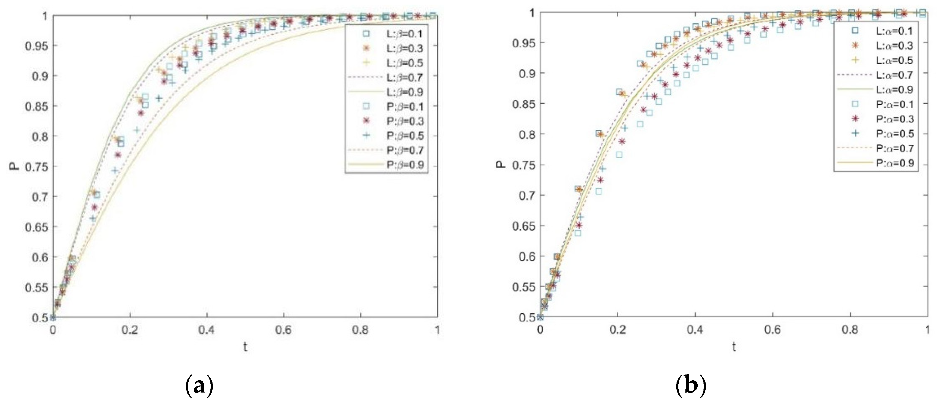
In this section, the MATLAB 2020a software is applied to simulate the initial probability value of the evolutionary system under different constraints and these parameters used in our model, for the purpose of verifying the accuracy of model consequences and making dynamic evolution trends more explicit and vivid. In addition, aiming at the ideal evolutionary stable state scenario 1, we simulate and analyze how the system evolves into ESS over time under the impact of different parameter changes. According to the basic assumptions and the interactive relationship between the parameters in scenario 1, scenario 2, scenario 3, and scenario 4, the relevant is set as shown in

Table 4. The initial values of the parameters.

Scenario	$\mathbf{\Delta }{\mathit{M}}_1$	$\mathbf{\Delta }{\mathit{M}}_2$	$\mathit{R}$	${\mathit{S}}_1$	${\mathit{S}}_2$	${\mathit{S}}_3$	${\mathit{C}}_1$	${\mathit{C}}_3$	${\mathit{C}}_4$	$\mathit{B}$	$\mathit{\alpha }$	$\mathit{\beta }$	$\mathit{K}$
Scenario 1	4	2	4	2	1	3	2	1	2	1	0.5	0.5	1
Scenario 2	4	2	4	2	1	1	5	1	2	4	0.5	0.5	1
Scenario 3	4	2	1	2	1	3	2	5	6	1	0.5	0.5	1
Scenario 4	1	2	4	1	2	3	1	3	6	0.5	0.7	0.3	1

.

For intuitively showing the dynamic evolution path and stable state in last mile delivery resource integration, the MATLAB2020a software is applied to simulate the dynamic evolutionary trajectories of the evolutionary system under different constraints and influencing factors. Aiming for the evolutionary stable state scenario 1, we simulate and analyze the impact of different parameter changes on the results. The parameters of diverse cases are set as shown in Table 4.

To begin with, we discuss the influence of initial behavioral strategy probability of LSPs, PSCs, and Cs on the ESS. Figure 4 shows the evolution path of the system, where the x, y, and z axes represent initial strategy probability values of LSPs, PSCs, and Cs, respectively. After giving the initial probability of their strategies, it can be seen that the system always evolves toward the stable state of {SI, SI, SSI}, and the larger the probability of initial value, the faster the speed of evolution. Similar to Figure 4a, the rate and stability of the system reaching equilibrium will also increase in Figure 4b–d, and the ESS are {SI, SI, STI}, {SI, TI, SSI}, and {TI, SI, SSI}, respectively. The simulation results verify correctness of the system evolution and stability strategy, as discussed above. It also shows that the greater willingness of the tripartite choosing the {SI, SI, SSI} strategy combination has a positive effect on the system in reaching evolutionary stability.

Next, we discuss the value changes of main parameters of {SI, SI, SSI}, involving profit allocation coefficient $\beta$, cost-sharing coefficient $\mathsf{\alpha }$, potential loss $S_i$, resource occupation compensation B, community premium profit K, parcel storage cost $C_1$, home delivery cost $C_3$, and integration cost $C_4$.

Based on the above simulation results, the initial policy probability of the tripartite has a certain impact on the rate at which the system reaches an equilibrium state, but there is no significant difference in the stability results of the system evolution. Therefore, without loss of generality, the initial strategy probabilities of the three parties are set to be x = 0.5, y = 0.5, and z = 0.5 in the following simulation.

5.1. Impact of $\beta$ and $\alpha$ on Evolutionary Outcome

Figure 5a,b show the impact of changing $\beta$ and $\mathsf{\alpha }$ on participation of LSPs and PSCs, respectively. The results are shown in Figure 5a: when $\beta$ is changed from 0.1 to 0.9, the speed of LSPs evolving to the SI strategy increases significantly, and PSCs’ declines. Furthermore, the difference in their willingness to choose the SI strategy is the smallest when $\beta =0.3$.

Figure 5b is opposite to Figure 5a; the speed of LSPs evolving to the SI strategy declines significantly, PSCs’ increases when $\mathsf{\alpha }$ is changed from 0.1 to 0.9, and the willingness of the two companies adopting the SI strategy is basically the same when α = 0.9. Thus, the result implies that there are optimal benefit allocation coefficients and cost-sharing coefficients in resource integration, which causes the ESS {SI, SI, SSI}.

5.2. Impact of $S_i$ on Evolutionary Outcome

Figure 6 depicts the impact of the variations $S_i$ on the participation of LSPs, PSCs, and Cs under the other parameters remain unchanged. In Figure 6a–c, we can see that the willingness of LSPs and PSCs in adopting the SI strategy and Cs in adopting the SSI strategy increase with the growth of $S_i$. At this time, LSPs and PSCs bear more cost of choosing the TI strategy, and Cs adopting the SSI strategy. Consequently, it shows a trend of the system evolving the stable state of {SI, SI, SSI}.

5.3. Impact of $B$ and $K$ on Evolutionary Outcome

Figure 7a,b illustrate how the level of B and K can influence the enthusiasm of Cs participating in the integration of delivery resources, respectively. It can be seen that given the growth of B, Cs tend to choose the STI strategy, but the willingness of PSCs adopting the SI strategy increases. When B > 4, $S_3$ generated by Cs choosing the STI strategy is less than B given by LSPs, and we obtain the ESS as {SI, SI, STI}. Based on Figure 7b, we find that the willingness of Cs adopting the SSI strategy is increased as the level of K increases.

The above analysis shows that the willingness of Cs in adopting the STI strategy reduces as the K increases. The reason is that K not enough to make up for the difference of B and $S_3$ when Cs receive excessive compensation due to unreasonable occupied public resources by the integration of LSPs and PSCs, which causes Cs to tend to choose the STI strategy. Nevertheless, Cs tend to choose the STI strategy, which causes their strategies to shift from the STI strategy to the SSI strategy.

5.4. Impact of $C_1$, $C_3$, and $C_4$ on Evolutionary Outcome

Figure 8 shows the willingness of LSPs and PSCs in participating in last mile delivery resources integration under changing $C_1$ paid by LSPs, $C_3$, and $C_4$, respectively. In Figure 8a, when the level of $C_1$ paid by LSPs increases, the enthusiasm of LSPs adopting the SI strategy rises, and PSCs are opposite. Due to the temporary package storage services provided by PSCs, they can obtain $C_1$. Furthermore, the enthusiasm of LSPs adopting the SI strategy can achieve greater as the level of $C_1$ increases. However, the enthusiasm of PSCs adopting the SI strategy reduces.

It can be seen from Figure 8b,c that with the increase in $C_3$ and $C_4$, the willingness of LSPs and PSCs in choosing the SI strategy decreases. In addition, we can see that PSCs are more sensitive to the costs changing in Figure 8. The reason is that PSCs are more sensitive to economic benefits in the last mile delivery, and they are inclined to balance costs and benefits. The reason is that PSCs show economic benefit sensitivity in the last mile delivery, and they prefer to weigh the costs and benefits.

6. Conclusions

Considering the dual roles of PSCs and Cs, we use evolutionary game theory to construct an evolutionary game model of last mile delivery resource integration among LSPs, PSCs, and Cs. In this game, the evolutionary stability of the strategic choice of tripartite participation in resource integration is analyzed, and the MATLAB2020a software is used to simulate the dynamic evolution of each game player and to analyze the impact of various related factors on the dynamic evolution of the system. Combined with the previous analysis, the main conclusions are as follows.

(1)

There are optimal profit allocation coefficients and cost-sharing coefficients that make the system evolve to a stable state of {SI, SI, SSI}. It shows that reasonable profit allocation and cost-sharing mechanisms are foundational, which guarantees the strategic integration between LSPs and PSCs. Therefore, the two companies should establish these mechanisms to ensure the stability of strategic integration.

(2)

Operating costs such as integration cost and home delivery cost could inhibit the strategic integration. Therefore, LSPs should take steps to improve Cs’ participation and try to establish a benign interactive relationship between themselves and customers to reduce the cost of strategic integration, such as creating logistics service member points systems, providing self-delivery, and delivery discounts.

(3)

The increasing of potential losses in temporary integration plays a positive role in promoting the evolution of the system to an ideal state of {SI, SI, SSI}, which indicates that the potential loss plays a vital role in the choice of strategic behaviors, and it requires the tripartite, especially the two types of enterprises, to establish a reasonable profit and loss evaluation system under different strategies to support scientific behavioral decisions before resource integration.

(4)

Higher community premium income is conducive to improving the enthusiasm of Cs supporting strategic integration. Therefore, while providing good logistics services, it is necessary for PSCs to improve the quality of property services through improving service attitudes and service standardization, so as to further improve community premium profits, and then encourage Cs to support strategic integration.

(5)

PSCs are more sensitive to the costs and benefits in the resource integration. Consequently, it is of great significance for the government to take measures to guide PSCs to actively participate in the last mile delivery resource integration by reducing their participation costs, such as providing financial subsidies and tax relief.

(6)

The three game players’ behavior and decision-making choices affect each other in the last mile delivery resource integration. Therefore, cooperation mechanisms and linkage relationships help to better integrate the last mile distribution resources.

(7)

The indirect benefits, such as advertising during their integration, play a positive role. Thus, the relevant regulations should be added in the property service contracts signed with Cs to avoid conflicts between Cs and PSCs by advertising and other acts.

References

1. Lewis, M.; Singh, V.; Fay, S. An Empirical Study of the Impact of Nonlinear Shipping and Handling Fees on Purchase Incidence and Expenditure Decisions. Mark. Sci. 2006, 25, 51–64. [Google Scholar] [CrossRef] [Green Version]
2. Zhou, L.; Lin, Y.; Wang, X.; Zhou, F. Model and algorithm for bilevel multisized terminal location-routing problem for the last mile delivery. Int. Trans. Oper. Res. 2019, 26, 131–156. [Google Scholar] [CrossRef]
3. Aized, T.; Srai, J.S. Hierarchical modelling of Last Mile logistic distribution system. Int. J. Adv. Manuf. Technol. 2014, 70, 1053–1061. [Google Scholar] [CrossRef]
4. Devari, A.; Nikolaev, A.G.; He, Q. Crowdsourcing the last mile delivery of online orders by exploiting the social networks of retail store customers. Transp. Res. Part E: Logist. Transp. Rev. 2017, 105, 105–122. [Google Scholar] [CrossRef]
5. Yang, F.; Yang, M.; Xia, Q.; Liang, L. Collaborative distribution between two logistics service providers. Int. Trans. Oper. Res. 2016, 23, 1025–1050. [Google Scholar] [CrossRef]
6. Hinterhuber, A. Can competitive advantage be predicted? Manag. Decis. 2013, 51, 795–812. [Google Scholar]
7. He, Y.; Wang, X.; Lin, Y.; Zhou, F.; Zhou, L. Sustainable decision making for joint distribution center location choice. Transp. Res. Part D Transp. Environ. 2017, 55, 202–216. [Google Scholar] [CrossRef]
8. Alnaggar, A.; Gzara, F.; Bookbinder, J.H. Crowdsourced delivery: A review of platforms and academic literature. Omega-Int. J. Manage. S. 2021, 98, 102–139. [Google Scholar]
9. Wang, X.; Zhan, L.; Ruan, J.; Zhang, J. How to Choose “Last Mile” Delivery Modes for E-Fulfillment. Math. Probl. Eng. 2014, 2014, 1–11. [Google Scholar]
10. Elhedhli, S.; Merrick, R. Green supply chain network design to reduce carbon emissions. Transp. Res. Part D Transp. Environ. 2012, 17, 370–379. [Google Scholar] [CrossRef]
11. Prajogo, D.; Olhager, J. Supply chain integration and performance: The effects of long-term relationships, information technology and sharing, and logistics integration. Int. J. Prod. Econ. 2012, 135, 514–522. [Google Scholar]
12. Panayides, P.M.; So, M. The impact of integrated logistics relationships on third-party logistics service quality and performance. Marit. Econ. Logist. 2005, 7, 36–55. [Google Scholar] [CrossRef]
13. Xu, X.; Zhang, W.; Li, N.; Xu, H. A bi-level programming model of resource matching for collaborative logistics network in supply uncertainty environment. J. Franklin. Inst. 2015, 352, 3873–3884. [Google Scholar] [CrossRef]
14. Yao, J. Decision optimization analysis on supply chain resource integration in fourth party logistics. J. Manuf. Syst. 2010, 29, 121–129. [Google Scholar] [CrossRef]
15. Cao, W.; Zhu, H. Supply Chain Integration Based on Core Manufacturing Enterprise. In International Conference on Computer and Computing Technologies in Agriculture; Springer: Berlin/Heidelberg, Germany, 2010; pp. 14–19. [Google Scholar]
16. Shi, X.; Li, L.X.; Yang, L.; Li, Z.; Choi, J. Information flow in reverse logistics: An industrial information integration study. Inform. Technol. Manag. 2012, 13, 217–232. [Google Scholar] [CrossRef]
17. Fan, T.; Pan, Q.; Pan, F.; Zhou, W.; Chen, J. Intelligent logistics integration of internal and external transportation with separation mode. Transp. Res. Part D Transp. Environ. 2020, 133, 101806. [Google Scholar] [CrossRef]
18. Adams, F.G.; Richey, R.G., Jr.; Autry, C.W.; Morgan, T.R.; Gabler, C. Supply chain collaboration, integration, and relational technology: How complex operant resources increase performance outcomes. J. Bus. Logist. 2014, 35, 299–317. [Google Scholar] [CrossRef]
19. Fan, Y.; Zhang, Y.; Song, Z.; Liu, H. Coordination Mechanism of Port Logistics Resources Integration from the Perspective of Supply-Demand Relationship. J. Coastal. Res. 2020, 103, 619–623. [Google Scholar]
20. Kim, S.T.; Lee, H.-H.; Hwang, T. Logistics integration in the supply chain: A resource dependence theory perspective. Int. J. Qual. Inno. 2020, 6, 1–14. [Google Scholar] [CrossRef]
21. Zhu, H.; Qiu, Y.; Jiang, T. Strategies for adopting unified object identifiers in logistics resource integration environments. J. Discret. Math. Sci. Cryptogr. 2018, 21, 991–1003. [Google Scholar] [CrossRef]
22. Yin, C.; Zhang, M.; Zhang, Y.; Wu, W. Business service network node optimization and resource integration based on the construction of logistics information systems. Inf. Syst. E-Bus. Manag. 2019, 18, 723–746. [Google Scholar] [CrossRef]
23. Chen, X.; Zhu, X.N. Logistics Infrastructure Network Evaluation Method Research Based on Logistics Resource Integration in Railway Logistics Enterprises. Adv. Mat. Res. 2014, 933, 941–946. [Google Scholar] [CrossRef]
24. Cruijssen, F.; Cools, M.; Dullaert, W. Horizontal cooperation in logistics: Opportunities and impediments. Transp. Res. Part E: Logist. Transp. Rev. 2007, 43, 129–142. [Google Scholar] [CrossRef] [Green Version]
25. Cruijssen, F.; Bräysy, O.; Dullaert, W.; Fleuren, H.; Salomon, M. Joint Route Planning under Varying Market Conditions. Int. J. Phys. Distrib. Logist. Manag. 2006, 49, 287–304. [Google Scholar] [CrossRef] [Green Version]
26. Zhou, L.; Baldacci, R.; Vigo, D.; Wang, X. A Multi-Depot Two-Echelon Vehicle Routing Problem with Delivery Options Arising in the Last Mile Distribution. Eur. J. Oper. Res. 2018, 265, 765–778. [Google Scholar]
27. Wang, Y.; Peng, S.; Guan, X.; Fan, J.; Wang, Z.; Liu, Y.; Wang, H. Collaborative logistics pickup and delivery problem with eco-packages based on time–space network. Expert Syst. Appl. 2021, 170, 114561. [Google Scholar]
28. Archetti, C.; Savelsbergh, M.; Speranza, M.G. The Vehicle Routing Problem with Occasional Drivers. Eur. J. Oper. Res. 2016, 254, 472–480. [Google Scholar] [CrossRef]
29. Chen, C.; Pan, S.; Wang, Z.; Zhong, R.Y. Using taxis to collect citywide E-commerce reverse flows: A crowdsourcing solution. Int. J. Prod. Res. 2017, 55, 1833–1844. [Google Scholar] [CrossRef]
30. Kafle, N.; Zou, B.; Lin, J. Design and modeling of a crowdsource-enabled system for urban parcel relay and delivery. Transp. Res. Part B Methodol. 2017, 99, 62–82. [Google Scholar] [CrossRef]
31. Macrina, G.; Di Puglia Pugliese, L.; Guerriero, F.; Laporte, G. Crowd-shipping with time windows and transshipment nodes. Comput. Oper. Res. 2020, 113, 104806. [Google Scholar]
32. Lyapunov, A.M. The General Problem of the Stability of Motion. J. Appl. Mech. 1994, 226–227. [Google Scholar] [CrossRef] [Green Version]
33. Selten, R. A note on evolutionarily stable strategies in asymmetric animal conflicts. J. Theor. Biol. 1980, 84, 67–75. [Google Scholar] [CrossRef] [Green Version]
Figure 1. Replicator dynamics phase diagram of LSPs. (a) y = y 0 ; (b) y > y 0 ; (c)   y < y 0 .
Sustainability 13 12240 g001
Figure 2. Replicator dynamics phase diagram of PSCs. (a) z = z 0 ; (b) z > z 0 ; (c)   z < z 0 .
Sustainability 13 12240 g002
Figure 3. Replicator dynamics phase diagram of Cs. (a) y = y 0 ; (b) y > y 0 ; (c)   y < y 0 .
Sustainability 13 12240 g003
Figure 4. Dynamic evolutionary paths of the system: (a) scenario 1; (b) scenario 2; (c) scenario 3; (d) scenario 4.
Sustainability 13 12240 g004
Figure 5. The impact of factors on evolution results: (a)   β ; (b)   α .
Sustainability 13 12240 g005
Figure 6. The impact of factors on evolution results: (a) S 1 ; (b)   S 2 ; (c) S 3 .
Sustainability 13 12240 g006
Figure 7. The impact of factors on evolution results: (a)   B ; (b)   K .
Sustainability 13 12240 g007
Figure 8. The impact of factors on evolution results: (a)   C 1 ; (b)   C 3 ; (c)   C 4 .
Sustainability 13 12240 g008